


ABSTRACT
Extensive rovibrational line lists were computed for nine isotopologues of the CO molecule, namely, 12C16O, 12C17O, 12C18O, 13C16O, 13C17O, 13C18O, 14C16O, 14C17O, and 14C18O in the ground electronic state with v ⩽ 41, Δv ⩽ 11, and J ⩽ 150. The line intensity and position calculations were carried out using a newly determined piece-wise dipole moment function (DMF) in conjunction with the wavefunctions calculated from an experimentally determined potential energy function from Coxon & Hajigeorgiou. A direct-fit method that simultaneously fits all the reliable experimental rovibrational matrix elements has been used to construct the dipole moment function near equilibrium internuclear distance. In order to extend the amount and quality of input experimental parameters, new Cavity Ring Down Spectroscopy experiments were carried out to enable measurements of the lines in the 4–0 band with low uncertainty as well as the first measurements of lines in the 6–0 band. A new high-level ab initio DMF, derived from a finite field approach has been calculated to cover internuclear distances far from equilibrium. Accurate partition sums have been derived for temperatures up to 9000 K. In addition to air- and self-induced broadening and shift parameters, those induced by CO2 and H2 are now provided for planetary applications. A complete set of broadening and shift parameters was calculated based on sophisticated extrapolation of high-quality measured data. The line lists, which follow HITRAN formalism, are provided as supplementary material.
Export citation and abstract BibTeX RIS
1. INTRODUCTION
Accurate spectroscopic parameters of carbon monoxide, including line position, line strength, Einstein A coefficient, and line-shape profiles are crucial for a variety of astrophysical applications. These parameters are needed in many carbon monoxide surveys which aid in our understanding of the thermodynamics of molecular clouds and stellar atmospheric structure (Dame et al. 2001; Thomas et al. 2006). The CO fundamental (1–0) band has proven to be a good quantitative tracer of molecular gas (Dame et al. 2001). These parameters are also useful in the study of the solar atmosphere structure, for example, the infrared rovibrational spectrum of CO is a valuable tracer for the thermal profile of the solar mid-photosphere, as pointed out by Thomas et al. (2006). Moreover, CO has been observed in the atmospheres of the planets Venus (Bezard et al. 1990) and Mars (Krasnopolsky 2014). One recent study of a massive exoplanet orbiting the star HR 8799 evidently reveals the existence of water and carbon monoxide in its atmosphere (Konopacky et al. 2013). The minor isotopologues of CO are important in understanding the evolution of various astrophysical objects. Black (2001) has mentioned the intriguing possibility of finding radioactive 14C in CO in novae, where nucleosynthesis and envelope formation occur on timescales shorter than the half-life, 5700 ± 30 yr.
Another major application that requires highly accurate line parameters of CO is the remote sensing of the terrestrial atmosphere, which often utilizes high-resolution spectrometers on board satellites, balloons, and ground-based instruments (Clerbaux et al. 2008; Rinsland et al. 2006; Liu et al. 2011, 2014). Atmospheric CO is considered as a pollutant and is mostly generated from biomass burning and fossil fuel combustion. It also plays an important role in the atmospheric carbon cycle (Crutzen et al. 1979). The line parameters of CO have been used to retrieve the production, concentration, and transport information from satellite spectra (Clerbaux et al. 2008; Rinsland et al. 2006).
Biomass burning shows CO emission features from highly excited rotational and vibrational states. The flame temperature, which can exceed 1300 K, is best determined with these CO hot-band features (4–3 band and above). The flame temperature is a valuable parameter for firefighting and the study of the impact of biomass burning on the atmosphere. A demand on the line parameters, particularly line intensities with accuracy better than 1%, is clearly mandated for a better interpretation of the spectra recorded for the terrestrial atmosphere using air-borne or satellite-borne instruments.
As one of the major infrared active absorbers in the atmosphere, the CO molecule was included in the very first version of the HITRAN database (McClatchey et al. 1973) and has been updated and expanded periodically. Since a major goal of the HITRAN database is to aid the remote-sensing of the terrestrial atmosphere, it has not included many hot bands and high vibrational and rotational levels. Although with adequate partition functions one should be able to scale these line parameters to obtain a good estimation of the absorption spectra at high temperature using Equation (1) given by Rothman et al. (2010), the missing hot bands that are not necessarily considered in HITRAN would be significant at high temperatures. To address this issue, an analogue database called HITEMP was created (Rothman et al. 1995). The intensities in the current CO line list in the HITEMP2010 database (Rothman et al. 2010) are largely based on Goorvitch 1994 and Goorvitch & Chackerian 1994a, 1994b, but supplemented with values from the Cologne Database for Molecular Spectroscopy (CDMS; Müller et al. 2005) in the MW region and newer experimental data for the 2–0 (Brault et al. 2003) and 3–0 (Sung & Varanasi 2004a) bands. The line positions of the current HITRAN2012 CO line list (Rothman et al. 2013) are largely based on the Dunham coefficients of Farrenq et al. (1991), but with the 0–0 band of 12C16O, 13C16O, and 12C18O, and the 1–1, 2–2, and 3–3 bands of 12C16O supplemented with the values from the CDMS database (Müller et al. 2005), the 0–0 band of 12C17O and 13C18O, and the 1–1 band of 13C16O, 12C18O, 12C17O, and 13C18O supplemented with data from Varberg & Evenson (1992). The intensities in Goorvitch (1994) and Goorvitch & Chackerian (1994a, 1994b) are based on the semi-empirical dipole moment function of Chackerian et al. (1994). This DMF is an updated version of the previously used Chackerian & Tipping (1983) DMF featuring the addition of intensity-ratio measurements for high vibrational levels. The Chackerian et al. (1984) DMF has incorporated the data of experimental line-intensity measurements prior to 1985. The current HITEMP CO line list consists of 113,631 lines, with Δv = 0, 1, 2, 3, 4, vMAX = 20, and JMAX = 150, where v, J are vibrational and rotational quantum numbers, respectively. The HITRAN2012 database is basically a reduced version of the HITEMP database with the minor exception that the 2–0 band for the three most abundant isotopologues contains updates using the studies of Malathy Devi et al. (2012a, 2012b). Since the minor isotopologue bands, except for the 2–0 band, still rely on the outdated semi-empirical dipole moment function in HITRAN and HITEMP, they create a discrepancy between isotopologues and can lead to incorrect spectroscopic derivations of relative abundances. For example, this inconsistency has been observed in cavity ring down spectroscopy (CRDS) work on the 3–0 band (Wójtewicz et al. 2013) where the measurements of the 3–0 lines for the principal isotopologue agreed well with HITRAN, while the measurements for the 4–1 and 3–0 bands of the minor isotopologues did not. This situation has a negative impact on the studies of the relative abundances of isotopic species, for instance, determining the ratio of oxygen isotopes in the solar atmosphere, see, for instance, Ayres et al. (2013).
In the literature, there are two rovibrational line lists most frequently used involving high v and J quantum numbers for the CO molecule for astrophysical applications (Goorvitch 1994; Hure & Roueff 1996). However, significant differences have been found between the reported line intensities of the two data sets. These large differences essentially arise from the different dipole moment functions used, which are a semi-empirical DMF from Chackerian et al. (1984) in the case of Goorvitch and a high-level ab initio DMF from Langhoff & Bauschlicher (1995, hereafter LB95) in the case of Hure and Roueff. It is not clear which study is better, which has caused some perplexity for potential users of the line lists. Both groups (Chackerian et al. 1994) argued that the semi-empirical DMF should be used preferentially to the ab initio one, and they concluded that more study is needed in the future to test both DMFs.
In the present study, we have constructed a semi-empirical DMF of CO using the best up-to-date experimental line intensity measurements from the pure rotational band up to the v' = 6 ← v'' = 0 band, where v' and v'' denote the upper and lower vibrational levels, respectively. Moreover, new measurements of the 4–0 band have been carried out at the University of Grenoble using the cavity ring down spectroscopic (CRDS) technique specifically to aid this study. In addition, the first measurement of the 6–0 band was carried out in Hefei using CRDS. The semi-empirical DMF has been constructed using a direct fit method that fits all the rovibrational matrix elements from different bands at once with appropriate weightings (see Li et al. 2011 for this methodology). High-level ab initio dipole moment points were employed to cover the long-range feature of the DMF. We argue that our semi-empirical DMF is superior to that of Chackerian et al. (1984), while our ab initio DMF is superior to that in LB95.
Although our semi-empirical DMF was constructed only using experimental and ab initio data for the principal isotopologue of carbon monoxide, it can be used to calculate intensities for all isotopologues if one neglects possible breakdown of the Born–Oppenheimer approximation. Combined with the spectroscopically determined mass-independent potential energy function from Coxon & Hajigeorgiou (2004), the line positions and intensities were calculated for all possible transitions with v ⩽ 41 and J ⩽ 150 of nine isotopologues of the electronic ground state of the CO molecule, namely, 12C16O, 12C17O, 12C18O, 13C16O, 13C17O, 13C18O, 14C16O, 14C17O, and 14C18O. The new line lists will be used to update line lists for CO in the current version of HITRAN (Rothman et al. 2013) and HITEMP (Rothman et al. 2010). In general, our new calculated line positions and intensities have been found to be in excellent agreement with the best available experimental values and have been shown to be a significant improvement over the previous HITRAN compilations, especially for the minor isotopologues.
The study of the CO abundance on planets with atmospheres which are predominantly composed of CO2, including Venus and Mars, or H2, such as gas giants, impose additional requirements on reference spectral databases. The correct interpretation of high-resolution infrared spectra of CO on Venus and Mars requires spectroscopic line parameters such as CO2-induced widths and shifts. To meet that requirement, the CO2 broadening and shifts have been measured, for instance, by Sung & Varanasi (2005) for the 1–0 band at three different temperatures, 201, 244, and 300 K, and for the 2–0 and 3–0 bands at 298 K. Similarly, inspired by many applications of H2-dominant environments, the H2 broadening and shift parameters for CO have also been studied (see for instance Malathy Devi et al. 2004, Sung & Varanasi 2004b, Régalia-Jarlot et al. 2005, Dick et al. 2009, Faure et al. 2013, and Padmanabhan et al. 2014). Here we created semi-empirically derived algorithms to provide these line-shape parameters for every line in the new data set.
The outline of this paper is as follows. Section 2 describes the new experiments of the 4–0 and 6–0 bands. Section 3 outlines the procedure for constructing the semi-empirical and ab initio DMFs and the comparison with previous studies. Section 4 details the line position calculation procedures. Section 5 is the results section which shows the comparison of the present study with experiments as well as with the HITRAN2012 and HITEMP2010 databases. Section 6 describes the development of line-shape parameters. Section 7 describes the format of the supplementary materials.
2. CAVITY RING-DOWN MEASUREMENTS FOR THE 4–0 AND 6–0 BANDS OF CO
2.1. Rovibrational Measurements of the 4–0 Band
Transitions of the 4–0 band were investigated in Grenoble with a newly developed cw-CRDS spectrometer using a fibered External Cavity Diode Laser (ECDL: Toptica DL pro, 1200 nm) as the light source. The total spectral coverage of this spectrometer is about 7900–8320 cm−1. High P(J) 4–0 lines are located in the high-energy part of this interval. They were measured one by one on the basis of their predicted line positions.
The set up is very similar to the CRDS spectrometer based on distributed feed back (DFB) which is used routinely in the 5850–7920 cm−1 region (Kassi & Campargue 2012; Tran et al. 2013). The 1.40 m long CRDS cell is fitted with high reflectivity mirrors leading to ring down times of about 200 μs. The CRDS cell was filled with carbon monoxide (Alphagaz 99% stated purity) at a pressure of 10.0 Torr. The pressure and the ring down cell temperature were monitored during the spectrum acquisition. The typical mode-hop free tuning range of this ECDL is about 0.8 cm−1. The laser frequency was tuned over a 1.6 cm−1 wide region around the line center by changing the grating angle together with the laser current. Three consecutive and partially overlapping spectra were typically recorded for each line. About 10 ring down events were averaged for each spectral data point separated by 8 × 10⁻⁴ cm−1. The noise equivalent absorption evaluated as the rms of the baseline fluctuation is better than αmin ∼ 1 × 10⁻¹¹ cm−1, as illustrated in Figure 1. An important advantage of this ECDL compared to the DFB diode lasers used in Kassi & Campargue (2012) and Tran et al. (2013) lies in its smaller frequency jitter (typically 100 kHz compared to 2 MHz), which limits the noise due to the conversion of the frequency jitter in intensity fluctuations on the rising and falling portions of a line profile.

Figure 1. Example of the CRDS measurement for the P(21) line of the 4–0 band of 12C16O.
Download figure:
Standard image High-resolution imageThe wavenumber of the light emitted by the laser diode was measured by a commercial Fizeau type wavemeter (HighFinesse WSU7-IR, 5 MHz resolution, 20 MHz accuracy over 10 hr) that allows laser frequency to be determined at a typical 100 Hz refresh rate. In order to further refine the absolute calibration, a very low pressure scan was recorded previous to this experiment, showing H2O lines (present as impurity) for which accurate line positions were taken from the HITRAN2008 database (Rothman et al. 2009). We estimate the accuracy of the absolute calibration of the wavenumber scale of our spectra at 1 × 10⁻³ cm−1.
In the line profile fitting, the ECDL line width contribution (FWHM) was neglected compared to the Doppler broadening (∼0.1 MHz and ∼0.57 GHz FWHM, respectively). In a first step, a Voigt function of the wavenumber was adopted for the line shape. The half width at half maximum (HWHM) of the Gaussian component was fixed to its theoretical value. The local baseline (assumed to be a linear function of the wavenumber), the line center, the integrated absorbance, and the HWHM of the Lorentzian component were fitted. Figure 1 shows the best reproduction of the P(21) line recorded at 10.0 Torr obtained with a Voigt profile. The W shape residual is a typical signature of the Dicke narrowing effect. Much reduced residuals were obtained using a Galatry line profile. Note that weak absorption lines due to water and carbon dioxide had to be taken into account in order to reproduce the spectrum.
In this way, the center and intensity of 10 P(J) 4–0 lines with J values between 19 and 34 were determined (Tables 1 and 2). They include the weakest CO lines that were ever measured quantitatively by absorption spectroscopy, such as the P(34) line with an intensity of about 1.9 × 10⁻³⁰ cm−1/(molecule × cm−2). (Note that these units are often given by their reduced form, cm molecule−1, but the longer version emphasizes the sense of wavenumber per column density.)
Table 1. CRDS Measurements of Line Positions for the 4–0 and 5–1 Bands of CO and Its Isotopologues in Units of cm−1
| Isotopologue | QN | PS(CRDS) | HITRAN 2012 | Δa | Tashkun et al. (2010) | Δb | Coxon & Hajigeorgiou (2004) | Δc |
|---|---|---|---|---|---|---|---|---|
| 4–0 band | ||||||||
| 12C16O | P(34) | 8206.1552 | 8206.1539 | −0.0013 | 8206.1540 | −0.0012 | 8206.1519 | −0.0033 |
| 12C16O | P(33) | 8214.5381 | 8214.5371 | −0.0010 | 8214.5370 | −0.0012 | 8214.5351 | −0.0030 |
| 12C16O | P(28) | 8254.4227 | 8254.4219 | −0.0007 | 8254.4218 | −0.0008 | 8254.4205 | −0.0021 |
| 12C16O | P(26) | 8269.4262 | 8269.4255 | −0.0008 | 8269.4254 | −0.0008 | 8269.4243 | −0.0020 |
| 12C16O | P(24) | 8283.8849 | 8283.8842 | −0.0007 | 8283.8841 | −0.0009 | 8283.8832 | −0.0017 |
| 12C16O | P(23) | 8290.9096 | 8290.9089 | −0.0007 | 8290.9089 | −0.0007 | 8290.9080 | −0.0016 |
| 12C16O | P(22) | 8297.7977 | 8297.7970 | −0.0007 | 8297.7969 | −0.0008 | 8297.7961 | −0.0016 |
| 12C16O | P(21) | 8304.5489 | 8304.5483 | −0.0006 | 8304.5482 | −0.0007 | 8304.5475 | −0.0014 |
| 12C16O | P(20) | 8311.1632 | 8311.1626 | −0.0006 | 8311.1625 | −0.0007 | 8311.1619 | −0.0013 |
| 12C16O | P(19) | 8317.6404 | 8317.6399 | −0.0005 | 8317.6397 | −0.0007 | 8317.6393 | −0.0011 |
| 12C18O | P(3) | 8206.0470 | 8206.0460 | −0.0010 | ||||
| 13C16O | R(6) | 8254.6879 | 8254.6870 | −0.0009 | ||||
| 12C17O | P(5) | 8290.4867 | 8290.4862 | −0.0005 | ||||
| 5–1 band | ||||||||
| 12C16O | P(9) | 8269.6394 | 8269.6385 | −0.0009 | 8269.6385 | −0.0009 | ||
| 12C16O | P(6) | 8283.9970 | 8283.9960 | −0.0010 | 8283.9961 | −0.0009 | ||
Notes. QN stands for quantum identification of the line, and PS stands for present study. aDifference between line positions from HITRAN and the CRDS measurements. bDifference between line positions generated from energy levels of Tashkun et al. (2010) and the CRDS measurements. cDifference between line positions from Coxon & Hajigeorgiou (2004) and the CRDS measurements.
Download table as: ASCIITypeset image
Table 2. CRDS Measurements of Line Intensities for the 4–0 and 5–1 Bands of CO and Its Isotopologues in Units of cm−1/(molecule × cm−2)
| Isotopologue | QN | PS(CRDS) | At 296 K | HITRAN 2012 | Δ%a | PS(fitted) | Δ%b | PS(ab initio) | Δ%c |
|---|---|---|---|---|---|---|---|---|---|
| 4–0 band | |||||||||
| 12C16O | P(34) | 1.902 × 10⁻³⁰ | 1.934 × 10⁻³⁰ | 1.770 × 10⁻³⁰ | −8.5% | 1.972 × 10⁻³⁰ | 2.0% | 2.049 × 10⁻³⁰ | 5.9% |
| 12C16O | P(33) | 3.756 × 10⁻³⁰ | 3.816 × 10⁻³⁰ | 3.378 × 10⁻³⁰ | −11.5% | 3.761 × 10⁻³⁰ | −1.4% | 3.903 × 10⁻³⁰ | 2.3% |
| 12C16O | P(28) | 6.987 × 10⁻²⁹ | 7.065 × 10⁻²⁹ | 6.365 × 10⁻²⁹ | −9.9% | 7.049 × 10⁻²⁹ | −0.2% | 7.285 × 10⁻²⁹ | 3.1% |
| 12C16O | P(26) | 1.971 × 10⁻²⁸ | 1.990 × 10⁻²⁸ | 1.791 × 10⁻²⁸ | −10.0% | 1.979 × 10⁻²⁸ | −0.6% | 2.042 × 10⁻²⁸ | 2.6% |
| 12C16O | P(24) | 5.096 × 10⁻²⁸ | 5.136 × 10⁻²⁸ | 4.648 × 10⁻²⁸ | −9.5% | 5.123 × 10⁻²⁸ | −0.3% | 5.280 × 10⁻²⁸ | 2.8% |
| 12C16O | P(23) | 7.974 × 10⁻²⁸ | 8.030 × 10⁻²⁸ | 7.261 × 10⁻²⁸ | −9.6% | 7.993 × 10⁻²⁸ | −0.5% | 8.231 × 10⁻²⁸ | 2.5% |
| 12C16O | P(22) | 1.222 × 10⁻²⁷ | 1.230 × 10⁻²⁷ | 1.111 × 10⁻²⁷ | −9.7% | 1.221 × 10⁻²⁷ | −0.7% | 1.257 × 10⁻²⁷ | 2.2% |
| 12C16O | P(21) | 1.827 × 10⁻²⁷ | 1.837 × 10⁻²⁷ | 1.665 × 10⁻²⁷ | −9.4% | 1.828 × 10⁻²⁷ | −0.5% | 1.880 × 10⁻²⁷ | 2.3% |
| 12C16O | P(20) | 2.672 × 10⁻²⁷ | 2.685 × 10⁻²⁷ | 2.442 × 10⁻²⁷ | −9.1% | 2.678 × 10⁻²⁷ | −0.3% | 2.752 × 10⁻²⁷ | 2.5% |
| 12C16O | P(19) | 3.827 × 10⁻²⁷ | 3.844 × 10⁻²⁷ | 3.508 × 10⁻²⁷ | −8.7% | 3.840 × 10⁻²⁷ | −0.1% | 3.945 × 10⁻²⁷ | 2.6% |
| 12C18O | P(3) | 5.709 × 10⁻²⁹ | 5.701 × 10⁻²⁹ | 5.673 × 10⁻²⁹ | −0.5% | 5.792 × 10⁻²⁹ | 1.6% | ||
| 13C16O | R(6) | 7.452 × 10⁻²⁸ | 7.447 × 10⁻²⁸ | 7.958 × 10⁻²⁸ | 6.9% | 8.674 × 10⁻²⁸ | 9.0% | ||
| 12C17O | P(5) | 1.665 × 10⁻²⁹ | 1.663 × 10⁻²⁹ | 1.514 × 10⁻²⁹ | −9.0% | 1.408 × 10⁻²⁹ | −7.0% | ||
| 5–1 band | |||||||||
| 12C16O | P(9) | 7.615 × 10⁻³⁰ | 7.613 × 10⁻³⁰ | 7.130 × 10⁻³⁰ | −6.3% | 7.351 × 10⁻³⁰ | −3.5% | ||
| 12C16O | P(6) | 7.920 × 10⁻³⁰ | 7.912 × 10⁻³⁰ | 8.171 × 10⁻³⁰ | 3.3% | 8.269 × 10⁻³⁰ | 4.5% | ||
Notes. QN stands for quantum identification of the line, and PS stands for present study. Natural isotopic abundance is assumed for our CRDS measurements. aPercentage difference between HITRAN and the CRDS measurements. bPercentage difference between the present semi-empirical intensities and the CRDS measurements. cPercentage difference between the present ab initio intensities and the CRDS measurements.
Download table as: ASCIITypeset image
During the spectra analysis, we found that a few additional CO lines were accidentally present in the spectral interval around the targeted 4–0 12C16O lines (see Tables 1 and 2). They include the P(6) and P(9) lines of the 5–1 hot band of 12C16O and one 4–0 line for each of the 13C16O, 12C18O, and 12C17O isotopologues present in natural abundance in the sample.
Tables 1 and 2 also list the line positions and intensities from the HITRAN database, and the semi-empirical and ab initio results of the present study for both the 4–0 and 5–1 bands. The observed line intensities have been converted to the intensities at 296 K using Equation (1) in the paper by Rothman et al. (2010). Discussion of these results in comparison with other sources of data is offered in Section 5.
2.2. Rovibrational Measurements of the 6–0 Band
The transitions of the 6–0 band of CO in the range of 12347–12497 cm−1 were recorded using a continuous wave cavity ring-down spectrometer (cw-CRDS). The experimental setup has been presented by Cheng et al. (2012). In brief, the 1 m long ring-down cavity is composed of two mirrors with a reflectivity of 99.995%. The spectral calibration is based on the frequencies of the passive modes of a Fabry–Perot interferometer (FPI) made of ultra-low-expansion glass. The 10 cm long FPI is placed in a vacuum chamber and thermo-stabilized. The absolute frequencies have been calibrated with an accuracy of about 2 MHz using the atomic transitions of 87Rb at 780 nm and 795 nm. The spectra were recorded at room temperature (296 ± 1 K), using sample pressures in the range of 0.2–0.8 atm. The gas pressure was measured by a capacitance gauge with a stated accuracy of 0.5%. The CO spectra of each line recorded at different pressures were fitted using a Voigt profile by fixing the Gaussian width at the calculated Doppler width. The positions, intensities, and Lorentzian widths were derived from the fitting. Here only the intensities of the R(5), R(7), R(9), and R(10) lines are presented in Table 3. The full analysis of this band will be presented in a separate study (Y. Tan et al. 2014, in preparation). Discussion of these results in comparison with other sources of data is offered in Section 5.
Table 3. CRDS Measurements of the Line Positions and Intensities for the 6–0 Band of 12C16O
| Line | Position (calculated) | Intensity/cm−1/(molecule × cm−2) | |||
|---|---|---|---|---|---|
| (cm−1) | PS (CRDS) | PS (fitted) | PS (ab initio) | LB95 (ab initio) | |
| R(5) | 12482.423741 | 9.17(28) × 10−29 | 9.18 × 10⁻²⁹ | 11.82 × 10⁻²⁹ | 1.344 × 10⁻²⁵ |
| R(7) | 12486.956652 | 9.20(19) × 10−29 | 9.11 × 10⁻²⁹ | 11.84 × 10⁻²⁹ | 1.416 × 10⁻²⁵ |
| R(9) | 12490.644870 | 7.74(21) × 10−29 | 7.85 × 10⁻²⁹ | 10.30 × 10⁻²⁹ | 1.299 × 10⁻²⁵ |
| R(10) | 12492.171852 | 6.95(12) × 10−29 | 6.97 × 10⁻²⁹ | 9.19 × 10⁻²⁹ | 1.190 × 10⁻²⁵ |
Download table as: ASCIITypeset image
3. CONSTRUCTION OF THE DIPOLE MOMENT FUNCTION
In 1984, Chackerian et al. (1984) reported a DMF for the X1Σ+ state of CO valid up to a large internuclear separation based on their intensity-ratio measurements for high vibrational levels. Their dipole moment function was later challenged by the high-level ab initio study by LB95, who found that their theoretical values deviate systematically from the intensity-ratio measurements at large internuclear separation, especially for v ⩾ 15. The high-level ab initio DMF (LB95) was obtained using the sophisticated averaged-coupled-pair functional (ACPF) method and an augmented correlation-consistent quadruple-zeta basis set (aug-cc-pVQZ). In 1994, based on the DMF of Chackerian et al. (1984), along with the transition frequencies by Farrenq et al. (1991), Goorvitch & Chackerian (1994a, 1994b) calculated the rovibrational line intensities of the seven most abundant isotopologues of CO for v ⩽ 20 and J ⩽ 150. Almost at the same time, Hure & Roueff (1996) generated another line list with intensities based on the ab initio DMF of LB95.
In the post-1994 era, a number of new highly accurate experimental measurements of the line intensities for the 0–0 through 3–0 bands became available (see, for instance, Birk et al. 1996; Jacquemart et al. 2001; Malathy Devi et al. 2012b and Zou & Varanasi 2002). The unprecedented accuracy of some of these studies was partly achieved by using non-Voigt line-shape profiles and accounting for line mixing. The importance of appropriate line shapes as well as accounting for line mixing is very well explained in Malathy Devi et al. (2012b). New measurements of the 4–0 band were discussed in the previous section. In addition, the observations of the previously unmeasured bands 4–1 (Wójtewicz et al. 2013), 5–0 (Chung et al. 2005), and 6–0 (Y. Tan et al. 2014, in preparation) had become available and allowed one to probe a larger range of internuclear distances. Along with the availability of the new accurate potentials from Coxon & Hajigeorgiou (2004), it seemed timely to incorporate the new information to update the DMFs of CO.
3.1. Semi-empirical Dipole Moment Function
Conventionally, the semi-empirical DMF is constructed based on the rotationless matrix elements Rv-0(m = 0), where v = 0, 1, 2, 3,...,vmax, and m = −J for P-branch lines and J + 1 for the R-branch lines. The rotationless matrix elements are determined by fitting the rotational matrix elements within a single vibrational band with a second-order polynomial function, which is known as the Herman–Wallis fit (Chackerian & Tipping 1983; Tipping & Ogilvie 1982). In our previous study (Li et al. 2011), we showed that it is possible to obtain the DMF by directly fitting all available rovibrational matrix elements with appropriate weightings of the experimental uncertainties. This method has been successfully applied to hydrogen halides, HF, HCl, HBr, and HI (Li et al. 2011, 2013a, 2013b). The direct-fit method is superior to the conventional method in the following ways: (1) it is now possible to obtain a good fit of a vibrational band using the high-precision measurements of just a few or even a single rotational line within that band, while a good Herman–Wallis fit needs substantially more lines covering both the P and R branches; (2) the overall accuracy and reliability of the fit has been improved by including more measurements from different studies and different bands with appropriate weightings; (3) better accounting for the rotational dependence is obtained than when only rotationless matrix elements are used.
The details of the direct-fit method have been explained in our previous study of the DMF of the HCl molecule (Li et al. 2011). A brief explanation is given as follows. First, the rovibrational matrix elements,  , are retrieved from the best available experimental measurements of rovibrational line intensities, using the equations in Šimečková et al. (2006). Here, double and single primes correspond to the lower and upper states, respectively. Second, the DMF (μ(r)) is usually approximated as a power series expansion (Bernath 2008)

where Mi are the coefficients of the polynomial expansion and x = (r − re)/re denotes the dimensionless Cartesian displacement with re as the equilibrium internuclear distance. Using this expansion,  can be rewritten as

At this stage, the determination of the Mi coefficients becomes a problem of solving the over-determined systems of equations, with the expectation values, 〈v'J'|xi|v''J〉, being calculated using the potential energy function. A weighted least-squares fit computer code by LeRoy (2004) has been accordingly modified to determine the Mi coefficients.
In the present study, the best spectroscopically determined potential energy functions of CO of Coxon & Hajigeorgiou (2004) have been employed to calculate the expectation values. We have also identified the best available line intensity measurements in the literature. In general, we used the measurements from Meerts et al. (1977) for the permanent dipole, Birk et al. (1996) for the pure rotational band, Zou & Varanasi (2002) for the fundamental band, Malathy Devi et al. (2012b) for the 2–0 band, Jacquemart et al. (2001) for the 3–0 band, our CRDS experiments in the 4–0 band described in Section 2, Chung et al. (2005) for the 5–0 band, and Y. Tan et al. (2014, in preparation) for the 6–0 band (also briefly described here in Section 2). A few individual rovibrational dipole moments for the 3–0 and 4–1 bands derived from intensities that were measured with lower uncertainty have also been added from the results of Wójtewicz et al. (2013). For the fundamental band, the results from Varanasi & Sarangi (1975) were not chosen because they have fitted the line intensities with a Voigt line-shape profile which could not resolve the line mixing properly. For the 3–0 band, there were two other different measurements that were carried out at a parallel time by Sung & Varanasi (2004a) and Chackerian et al. (2001). Interestingly, recent accurate measurements of high-J lines by Wójtewicz et al. (2013) could be fitted very well together with Jacquemart et al. (2001), while it was not in accord with the Sung & Varanasi (2004b) and Chackerian et al. (2001) data. Therefore the latter two sources were not included in the fit, although the differences were only of the order of 2%. A sequence of signs of dipole moment matrix elements (−+−+−−+) for the 0–0 through 6–0 bands was adopted to imply the C−O+ polarity as used in previous studies (Chackerian & Tipping 1983; Chackerian et al. 1984). It is interesting to note that the dipole moment matrix element flips its sign from R(16) − to R(17) + transitions of the 5–0 band as shown in Figure 2.

Figure 2. Calculated matrix elements for the 5–0 band of CO using the present semi-empirical DMF and the PEF of Coxon & Hajigeorgiou (2004).
Download figure:
Standard image High-resolution imageUltimately, a grand fit with appropriate weightings (taking into account experimental uncertainties) has been performed, and the Mi coefficients determined from the present study and the other studies are listed in Table 4. For the reader's reference, the input rovibrational matrix elements and the corresponding expectation values can be found in Table S1. First of all, we can see from Table 4 that two extra coefficients, M5 and M6, have been determined owing to the availability of intensity measurements of the 5–0 and 6–0 bands. Second, the M0, M1, M2, and M3 coefficients from the present study agree well with the ones from Chackerian & Tipping (1983). Nevertheless, the present power series expansion of the DMF is the most accurate, up-to-date one and should be superior to the ones determined by Chackerian & Tipping (1983) as a consequence of the new accurate experimental data. In addition, the present study should serve well as a reference for ab initio studies near equilibrium internuclear distance. Finally, we can see that the M2, M3, and M4 coefficients from Kiriyama & Rao (2000) do not agree with either Chackerian & Tipping (1983) or the present study, especially for the M2 coefficient, which is approximately an order of magnitude smaller than the other two studies. The likely reason for this is that Kiriyama & Rao (2000) failed to identify the best experimental measurements of line intensities and used only pre-1980s experimental data in their fitting.
Table 4. Coefficients of the Power Series Expansion of the DMFs of CO (in Debye)
| PS (fitted) | Kiriyama & Rao | Chackerian & Tipping | |
|---|---|---|---|
| (2000) | (1983) | ||
| M0 | −0.1229099(469) | −0.122861(4) | −0.122706 |
| M1 | 3.604742(720) | 3.614784(1305) | 3.63579 |
| M2 | −0.23716(103) | −0.031838(227) | −0.249088 |
| M3 | −3.67326(239) | −2.919004(882) | −3.54159 |
| M4 | 1.4892(812) | 4.214029(1774) | 2.57239 |
| M5 | 1.8293(1877) | ||
| M6 | −4.342(3885) |
Notes. PS stands for present study. Numbers in parentheses are the estimated standard deviations in units of the last significant digit of the corresponding coefficient.
Download table as: ASCIITypeset image
3.2. Ab Initio Dipole Moment Function
Experimental measurements for the intensities of high overtone bands are difficult due to the fact that these transitions are usually very weak. Ab initio calculation can provide a global DMF as a complement to the semi-empirical DMF. Therefore, it is desirable to compare and combine the two methods, i.e., the semi-empirical method described in Section 3.1 with the ab initio method, in order to cover the entire range of meaningful internuclear distances. In the present study, the best DMF of CO is presented as a piecewise function consisting of two parts: μ1 equals the semi-empirical calculation near equilibrium internuclear distance covering up to v = 6, while μ2 equals the ab initio DMF up to r = 4 a0, where a0 is the Bohr radius.
Langhoff & Bauschlicher (1995) have studied the DMF for the ground state of CO as a function of one and n-particle treatment. Their best calculated DMF using the finite-field approach has been found to be far superior to the ones calculated as expectation values. For evaluation purpose, we have employed their theoretical DMF to calculate the rovibrational line intensities of CO. The work has been carried out using the LEVEL program (LeRoy 2007) by combining the DMF with a PEF from Coxon & Hajigeorgiou (2004). A cubic spline function has been used to interpolate the dipole moment points from LB95. It has been found that the calculated line intensities for the 0–0 to 3–0 bands are in excellent agreement with the ones derived from the semi-empirical DMF of the present study (differences ⩽ 2%). However, unexpected large discrepancies have been found for the 4–0 and 5–0 bands, by approximately 20% and 80%, respectively, which are much larger than the reported experimental uncertainties used for fitting. Because of the excellent agreement for the 0–0 through 3–0 bands, we were perplexed about the discrepancies for the 4–0 and 5–0 bands until we re-calculated the DMF using the same approach as LB95 but with a finer grid (with a bond length interval of 0.02 a0 instead of 0.1 a0). When the new DMF was used to calculate the line intensities, the results for the 4–0 and 5–0 bands were in much better agreement with our semi-empirical values. The differences between the calculated and semi-empirical values at the band origin are now 2% and 10% for the 4–0 and 5–0 bands, respectively. Meanwhile, the new calculated line intensities for the 0–0 to 3–0 bands are almost identical to the previous calculated ones using the DMF of LB95. This gives us a hint that the interpolation method may not be sufficiently accurate at certain internuclear distances where the DMF behaves irregularly. Prior study also suggests that the intensity calculation is sensitive to the small change of the DMF at certain bond lengths (Li et al. 2013b). Therefore, we conclude that a finer grid of DMF should be a safer choice for quantitative studies in order to reproduce accurate line intensities.
LB95 carried out a calibration study to determine the sensitivity of the dipole moment to improvements in both the one- and n-particle basis sets. To do this, they selected two internuclear distances: 2.1 a0, which is near re, and 3.7 a0, which is near the maximum of the DMF. Although their best dipole moment agrees within 0.001 Debye with the one deduced from the semi-empirical DMF at 2.1 a0, the difference at 3.7 a0 is as large as 0.04 Debye. In addition, due to the limitation of computer power, they were not able to finish a number of more sophisticated calculations, leaving some gaps in their calibration table. In this work, we have extended their calibration study with more reference points at different internuclear distances and extended the size of the CASSCF/ACPF calculations further to (200/533) and (200/644) active space with the aug-cc-pVXZ basis set, where X = T, Q, 5 (abbreviated as AVXZ hereafter). For the new calculation, we have selected points at r = 2.1, 2.23, 2.30, 2.36, 2.41, 2.46, 3.70 a0, which are approximately re and the classic turning points for v = 0–4 and v = 40, respectively. Our newly calculated dipole moments at various internuclear distances using the finite-field approach, together with the corresponding values from LB95 are listed in Table 5. We can see from the table, first of all, that the results at 2.1 and 3.7 a0 from LB95 are almost identical to our newly calculated values. Second, poorer agreement has been found between experiment and calculation when the active space has been increased from (300/322) to (200/644). The difference between the values calculated using active space (300/322) and (200/533) is very small (<0.00005 atomic units (A.U.)). It has been found that the line intensities calculated using (300/322) agree better with experiments than the ones using (200/533) active space. Finally, systematic improvement has been seen when increasing the basis set from QZ to 5Z, with a difference in dipole moment between 0.0001 and 0.004 A.U., as shown in Figure 3. Considering the above three findings, the DMF has finally been calculated using the active space (300/322) and a basis set at 5Z level.

Figure 3. Ab initio DMF (in atomic units) calculated using the finite-field approach with the ACPF method and QZ/5Z basis sets (upper panel). Difference between the two DMFs (lower panel).
Download figure:
Standard image High-resolution imageTable 5. Validation Calculation for the X1Σ+ CO Dipole Moment (A.U.) Using the Finite-field Method with a Field Strength of ±0.005 A.U.
| Bond Length (Bohr) | Closed/Active Space | Basis Set | PS(fitted) | Ab initio (AV5Z)-PS(fitted) | ||
|---|---|---|---|---|---|---|
| AVTZ | AVQZ | AV5Z | ||||
| 2.10(re) | 300/322 | −0.07380 (−0.07382) | −0.07046 (−0.07046) | −0.06964 | −0.06960 | −0.00004 |
| 300/422 | −0.07732 | −0.07396 | −0.07315 | −0.06960 | −0.00355 | |
| 200/533 | −0.07413(−0.07413) | −0.07046 | −0.06951 | −0.06960 | 0.00009 | |
| 200/644 | −0.07281 | −0.06911 | −0.06814 | −0.06960 | −0.00146 | |
| 2.23(v = 0) | 300/322 | 0.01185 | 0.01585 | 0.01681 | 0.01587 | 0.00094 |
| 300/422 | 0.01009 | 0.01241 | 0.01336 | 0.01587 | −0.00251 | |
| 200/533 | 0.01136 | 0.01571 | 0.01679 | 0.01587 | 0.00092 | |
| 200/644 | 0.01280 | 0.01719 | 0.01832 | 0.01587 | 0.00245 | |
| 2.30(v = 1) | 300/322 | 0.05720 | 0.06161 | 0.06265 | 0.06110 | 0.00155 |
| 300/422 | 0.05544 | 0.05817 | 0.05921 | 0.06110 | −0.00189 | |
| 200/533 | 0.05657 | 0.06133 | 0.06250 | 0.06110 | 0.00140 | |
| 200/644 | 0.05808 | 0.06290 | 0.06411 | 0.06110 | 0.00301 | |
| 2.36(v = 2) | 300/322 | 0.09538 | 0.10033 | 0.10128 | 0.09914 | 0.00214 |
| 300/422 | 0.09363 | 0.09672 | 0.09945 | 0.09914 | 0.00031 | |
| 200/533 | 0.09461 | 0.09974 | 0.10098 | 0.09914 | 0.00184 | |
| 200/644 | 0.09619 | 0.10139 | 0.10268 | 0.09914 | 0.00354 | |
| 2.41(v = 3) | 300/322 | 0.12661 | 0.13170 | 0.13289 | 0.13021a | 0.00268 |
| 300/422 | 0.12486 | 0.12990 | 0.13107 | 0.13021 | 0.00086 | |
| 200/533 | 0.12571 | 0.13115 | 0.13246 | 0.13021 | 0.00225 | |
| 200/644 | 0.12735 | 0.13287 | 0.13423 | 0.13021 | 0.00402 | |
| 2.46(v = 4) | 300/322 | 0.15720 | 0.16263 | 0.16388 | 0.16066 | 0.00322 |
| 300/422 | 0.15547 | 0.15912 | 0.16037 | 0.16066 | −0.00029 | |
| 200/533 | 0.15617 | 0.16193 | 0.16331 | 0.16066 | 0.00265 | |
| 200/644 | 0.16372 | 0.16515 | 0.16066 | 0.00449 | ||
| 3.70(v = 40) | 300/322 | 0.57806 (0.57806) | 0.59087 (0.59087) | 0.59465 | 0.6448a | 0.050 |
| 300/422 | 0.56993 | 0.58271 | 0.58655 | 0.6448a | 0.058 | |
| 200/533 | 0.59071 (0.59070) | 0.60473 (0.60472) | 0.60886 | 0.6448a | 0.036 | |
| 200/644 | 0.58877 | 0.6448 | ||||
Notes. The corresponding values from Langhoff & Bauschlicher (1995) are in parentheses. aThese values are derived from the semi-empirical DMF of Chackerian et al. (1984).
Download table as: ASCIITypeset image
For the finite-field approach, a small artificial perturbation is introduced by adding an external electric field. To investigate the effect of the field strength, we have calculated the dipole moment at three different field strength values of ±0.0001, ±0.003, ±0.005 A.U. at the internuclear distance re = 2.13222 a0 using the ACPF(300/322) method plus a 5Z basis set. The calculated dipole moments are −0.04794, −0.04804, and −0.04812 A.U. at the three field strengths, respectively. Therefore, for the CO molecule, the choice of field strength does not affect the results very much (Δ ⩽ 0.0001 A.U.). In the present study, a field of 0.005 A.U. has been chosen for the rest of the calculations.
Another useful measure of the quality of the calculation is the rotationless matrix elements, Rv-0(0), which are proportional to the square root of the line intensities. LB95 have compared their ab initio Rv-0(0), where v = 0, 1, 2, 3, and 4, with the semi-empirical ones reported by Chackerian & Tipping (1983). They have found good agreement between the two studies, except for R4–0(0) where the difference is approximately 12%. In Table 6, we have carried out a similar comparison by adding the Rv-0(0) values calculated using both the semi-empirical and ab initio DMFs of the present study. As can be seen from this table, the theoretical R1–0 and R2–0 of LB95 agree better with the present semi-empirical study than the previous semi-empirical study of Chackerian & Tipping (1983). This suggests that for the 1–0 and 2–0 bands, the theoretical DMF of LB95 is actually of better quality than the semiempirical DMF of Chackerian & Tipping (1983).
Table 6. Rotationless Matrix Elements Rv0 in Debye
| Rv-0(m) | Chackerian & Tipping (1983) | Langhoff & Bauschlicher (1995) | PS (fitted) | PS (ab initio) |
|---|---|---|---|---|
| R0–0(0) | −0.11019 | −0.1117 | −0.11013 | −0.1117 |
| R1–0(0) | 0.10634 | 0.1077 | 0.10746 | 0.1076 |
| R2–0(0) | −6.6698 × 10−03 | −6.53 × 10−03 | −6.5431 × 10−03 | −6.54 × 10−03 |
| R3–0(0) | 4.2756 × 10−04 | 4.14 × 10−04 | 4.1213 × 10−04 | 4.15 × 10−04 |
| R4–0(0) | −2.0131 × 10−05 | −2.24 × 10−05 | −2.0744 × 10−05 | −2.09 × 10−05 |
| R5–0(0) | 5.1311 × 10−06 | −2.07 × 10−07 | −1.0160 × 10−06 | −1.08 × 10−06 |
| R6–0(0) | −3.0202 × 10−06 | 2.48 × 10−05 | 7.017 × 10−07 | 7.88 × 10−07 |
Note. PS stands for present study.
Download table as: ASCIITypeset image
For R0–0(0), R1–0(0), R2–0(0), and R3–0(0), the values calculated using the present ab initio DMF are almost identical to those from LB95. However, for R4–0(0), R5–0(0), and R6–0(0), the values from the present ab initio DMF are in much better agreement with the present semi-empirical values than those from LB95. With that, we note that the extreme disagreement between LB95 and our fitted and ab initio values for R6–0(0) (and to a lesser extent R5–0(0)) is not only an indication that ab initio calculation is better but largely due to the fact that one needs to calculate DMF points at a finer grid, especially at internuclear distances corresponding to higher overtones. The R6–0(0) value that we calculated from LB95 had proven to be extremely sensitive to the interpolation methods used and varied by orders of magnitude. We picked this particular interpolation to present here as it yielded the best results everywhere except for the R6–0(0) value.
Chackerian et al. (1994) raised their concern about the quality of the semi-empirical DMF of Chackerian & Tipping (1983) and the ab initio DMF of LB95 because of the large differences between the intensities calculated using these two DMFs. With the availability of the new CRDS measurement of the 6–0 band (Y. Tan et al. 2014, in preparation, see Table 3), we decided to test both ab initio DMFs by comparing the calculated line intensities using these two DMFs. In Table 3, the line intensities calculated using the present ab initio DMF are approximately 30%–38% higher than measurements of Y. Tan et al. (2014, in preparation), those calculated using LB95 by about three orders of magnitude, while the one calculated from the DMF of Chackerian & Tipping (1983) overestimated the line intensities by about fivefold (the latter not shown). It can thus be concluded that the DMF of Chackerian & Tipping (1983) is less accurate at larger internuclear distance.
4. CALCULATION OF LINE POSITIONS AND PARTITION FUNCTIONS
In 2012, Velichko et al. (2012) generated a set of accurate mass-independent Dunham-type parameters which globally described all rovibrational energy levels of the CO molecule (for six isotopologues). In their fit, a total number of 19,000 experimental transitions of seven isotopologues of CO collected from the literature were included. Earlier in 2004, Coxon & Hajigeorgiou (2004) adopted a different approach, which is called a parameterized Morse/Lennard-Jones (MLJ) potential, to interpret practically the same experimental data. After Velichko's paper was published, Coxon & Hajigeorgiou (2013) compared their calculated line positions with the ones from Velichko et al. (2012). Good agreement has been found between calculations that employ these two approaches. Considering that the parameterized potential usually has a better predictability for high-J lines, the mass-independent potential energy functions of Coxon & Hajigeorgiou (2004) have been employed in this work to calculate the line positions and lower-state energies for nine isotopologues using the LEVEL program (LeRoy 2007).
Partition sums, Q(T), for all nine isotopologues were also calculated for temperatures ranging from 1 to 9000 K by direct summation of all the calculated energy levels up to dissociation. The complete list of the derived partition sums can be found in the supplementary material. Given the high accuracy of spectroscopically determined energy levels, our new determination should be more accurate than previously reported ones. Table 7 compares the Q values derived from the present study with the ones used for the HITRAN and HITEMP databases (essentially calculated using the TIPS, Total internal partition sum, 2003 program (Fischer et al. 2003), the ones from the CDMS database (Müller et al. 2005), the ones calculated using the TIPS 2011 program (Laraia et al. 2011), and the ones calculated by (Goorvitch 1994)) at eight different temperatures, 9.375, 225, 296, 300, 1000, 3000, 6000, and 9000 K. At 9.375, 225, 296, and 300 K, the Q values from the present study are identical to the ones from the CDMS database, while the ones used in the HITRAN and HITEMP databases are 0.3% smaller than both CDMS and the present study. The values calculated using the TIPS 2011 program are in between the ones from the present study and the ones used for the HITRAN and HITEMP databases. At 1000 K, the Q value from the present study is identical to the Goorvitch value, while the value calculated using the TIPS 2011 program is 0.5% higher than both. Meanwhile, the Q value is largely underestimated in the CDMS database (by 5.6% at 1000 K). At 3000 K, the Q values from the present study are in excellent agreement with the ones derived by Goorvitch, while the value used in the HITRAN and HITEMP databases are approximately 0.18% larger than the present study. The value calculated using the TIPS 2011 program is larger than the present study by 1.6%. At 6000 and 9000 K, the Q values from the present study are smaller than Goorvitch values by 0.016% and 0.83%, respectively. In general, the Q values from the present study are identical to the ones in the CDMS database below 300 K, and are in excellent agreement with Goorvitch values above 1000 K. Therefore, we recommend using the present calculated Q values to replace the ones used in the HITRAN and HITEMP databases.
Table 7. Comparison of the Partition Function Q(T) of 12C16O
| T | This Work | Müller et al. 2005/CDMS | Fischer et al. 2003/TIPS 2003 | Laraia et al. 2011/TIPS 2011 | Goorvitch (1994) |
|---|---|---|---|---|---|
| (K) | (0–9000 K) | (0–1000 K) | (70–3000 K) | (70–3000 K) | (1000–10000 K) |
| 9.375 | 3.744 | 3.744 | |||
| 225 | 81.718 | 81.715 | 81.457 | 81.540 | |
| 296 | 107.420 | 107.117 | 107.259 | ||
| 300 | 108.868 | 108.868 | 108.563 | 108.711 | |
| 1000 | 380.297 | 362.660 | 380.453 | 382.191 | 380.3 |
| 3000 | 1717.244 | 1720.468 | 1744.216 | 1717.2 | |
| 6000 | 5643.574 | 5644.5 | |||
| 9000 | 12082.036 | 12187.2 |
Download table as: ASCIITypeset image
5. COMPARISONS OF LINE POSITIONS AND INTENSITIES FROM DIFFERENT SOURCES
5.1. Overview of the Available Databases
We have compiled a complete database of rovibrational transitions of nine isotopologues of carbon monoxide including radioactive ones. The extent of the database is given in Table 8. We originally calculated substantially larger data sets with transitions with Δv up to 41. However, using validation tools developed by Medvedev (2012), it was found that the intensities calculated for lines with Δv ⩾ 12 are unreliable. At the moment, it is unclear if this is due to any unforeseen problem with ab initio calculation at these internuclear distances or the numerical approach implemented by LEVEL. This will have to be determined in a separate study, probing several molecular systems. Nevertheless, the database with Δv ⩽ 11 is complete for any practical application. The intensities go down to 10−200 cm molecule−1 to accommodate even the most challenging high-temperature applications. For terrestrial and planetary atmosphere applications, it is informative to compare the calculated line positions and line intensities of the present study with experimental measurements as well as the ones in the HITRAN and HITEMP databases. Table 8 compares the present CO line lists with the HITRAN and HITEMP databases, and the Goorvitch data sets. We can see that the present study provides more comprehensive v, J, and Δv coverage, plus data for three additional radioactive isotopologues. To visualize the difference, the present line list (black square), HITEMP2010 (blue circle), and HITRAN2012 (red triangle) are plotted in Figure 4. The lower panel of this figure covers a spectral range of 0–70000 cm−1, with the line intensities plotted on logarithm scale. The upper panel is a blow up that covers all the Δv = 0–6 bands.

Figure 4. Overview of the line lists from the present semi-empirical study, the HITEMP2010, and the HITRAN 2012 databases. The top panel zooms on the spectral region up to the 6–0 band.
Download figure:
Standard image High-resolution imageTable 8. Summary Comparison of CO Rotation-Vibration Line Lists
| This Work | HITEMP 2010 | HITRAN 2012 | Goorvitch (1994) | |
|---|---|---|---|---|
| Stable isotopologues | 6 | 6 | 6 | 6 |
| Maximum v'' | 41 | 20 | 4 | 20 |
| Maximum J'' | 150 | 149 | 94 | 149 |
| Maximum Δv | 11 | 4 | 4 | 3 |
| Temperature range (K) | 1–9000 | 70–3000 | 70–3000 | 500–10000 |
| Spectral range (cm−1) | 2–22149 | 3–8464 | 3–8464 | 849–6417 |
| Number of lines | 752976 | 113631 | 4606 | 113022 |
| Radioactive | ||||
| isotopologues | 3 | None | None | None |
| Maximum v'' | 41 | |||
| Maximum J'' | 150 | |||
| Maximum Δv | 11 | |||
| Temperature range (K) | 1–9000 | |||
| Spectral range (cm−1) | 2–21293 | |||
| Number of lines | 376488 |
Download table as: ASCIITypeset image
5.2. Comparison with the HITRAN Database
The current version of the HITRAN database for CO consists of 4606 lines belonging to six isotopologues covering a spectral range of 3.46–8464.88 cm−1. In general, six vibrational bands 1–0, 2–0, 2–1, 3–0, 3–1, and 4–1 are included for the first six isotopologues; two pure rotational bands 0–0 and 1–1 are included for the first five isotopologues; and the 2–2, 3–3, and 4–0 bands are included only for the principal isotopologue. The line positions of the current HITRAN CO line list are largely based on the Dunham coefficients of Farrenq et al. (1991), but with the 0–0 band of 12C16O, 13C16O, and 12C18O, and the 1–1, 2–2, and 3–3 bands of 12C16O supplemented with the values from the CDMS database (Müller et al. 2005) and the 0–0 band of 12C17O and 13C18O, and the 1–1 band of 13C16O, 12C18O, 12C17O, and 13C18O supplemented with data from Varberg & Evenson (1992). Figure 5 shows the comparison of line positions of 12C16O between the HITRAN 2012 database and the present study which uses the PEF of Coxon & Hajigeorgiou (2004). For the pure rotational bands, 0–0, 1–1, 2–2, and 3–3, excellent agreement has been found between the two data sets for lines with J'' < 50. However, for the 0–0 band with J'' > 50, the HITRAN database starts to quickly diverge from the present study. For the 1–0 to 4–0 vibrational bands, the HITRAN database agrees very well with the present study near band origins but diverges quadratically for high-J lines, reaching differences of 0.0011, 0.0024, 0.0039, and 0.0063 cm−1 at J'' = 49, respectively, for the four vibrational bands. Similar comparison is also shown for the 2–1, 3–1, and 4–1 hot bands in Figure 5, with line position differences of 0.0013, 0.0028, 0.0042 cm−1 at J'' = 49, respectively. In general, the line positions from the present study are superior to the HITRAN database through the inclusion of new high-precision data for various CO isotopologues that were not contained in Farrenq et al. (1991) and through better predictability of the parameterized potential energy function for high-J lines.

Figure 5. Comparison of the line positions of 12C16O between the HITRAN2012 database and the present study which uses the PEF of Coxon & Hajigeorgiou (2004).
Download figure:
Standard image High-resolution imageHowever, a possible minor problem may still exist in the available line position data. As one of the illustrations, one can take a look at the comparisons of different data sets and measurements in the 4–0 and 5–1 bands carried out in this work. It can be seen that for the 4–0 band, the line positions in HITRAN agree well with the CRDS measurements. However, the agreement for calculated values using the potential energy function of Coxon & Hajigeorgiou (2004) is slightly worse, and moreover exhibits a definite rotational dependence reaching a maximum difference of 0.0034 cm−1 for the P(34) line. In 2010, Tashkun et al. (2010) carried out a Ritz analysis of 12C16O rovibrational energy levels that were involved in multiple (and often multiply) measured transitions. We generated transition frequencies from these energy levels and it appears that they also agree better with experimental ones than our values calculated based on the PEF of Coxon & Hajigeorgiou (2004). Nevertheless, the differences are marginal even at high-J values. For the 5–1 band, our line positions and those generated from the energy levels by Tashkun et al. (2010) are similar to each other and agree better with experimental values more than those for the 4–0 band. More high-precision experiments are desirable to improve existing line position analyses. On the other hand, the current line positions from any of the existing sources are of acceptable quality for most present-day applications.
The line intensity of the current HITRAN line list for CO was originally derived from the DMF of Chackerian & Tipping (1983), and was later replaced with the Goorvitch data sets (Goorvitch 1994; Goorvitch & Chackerian 1994a, 1994b). Recent (post 2000) updates to HITRAN for line intensity include the replacements for the pure rotational bands, 0–0, 1–1, 2–2, and 3–3, with the CDMS database (Müller et al. 2005), the 2–0 band with Malathy Devi et al. (2012a, 2012b), and the 3–0 band with Sung & Varanasi (2004a). Figure 6 shows the comparison of line intensities for the 0–0 to 6–0 bands of 12C16O between the experimental measurements, the HITRAN 2012 database, the ones calculated using the present ab initio DMF, and the ones calculated from the present semi-empirical DMF.

Figure 6. Comparison of line intensities of 12C16O rovibrational bands with the present semi-empirical study as a reference. m equals–J for P branch and J +1 for R branch lines. Note the different scales in the panels of the plot. PS refers to semi-empirical (fitted) or measured (CRDS) results from the present study. The 6–0 band intensities from LB95 study are three orders of magnitude off from the experimental measurements and are not given in this figure.
Download figure:
Standard image High-resolution imageAccording to this figure, for the 0–0 band, the present semi-empirical intensities (referred to as PS(fitted)) agree well with the four sets of measurements of Birk et al. (1996). Similar agreement has also been found between HITRAN and Birk et al. (1996), which is expected since the same data from Birk et al. (1996) were adopted in HITRAN. The line intensities for the 0–0 band derived from the ab initio DMFs of both the present study (referred to as PS(ab initio)) and LB95 differ from the semi-empirical values by approximately −1% and +3%, respectively.
For the 1–0 band, the PS(fitted) intensities agree well with the measurements of Zou & Varanasi (2002) within the reported uncertainty except for a few high-J, R-branch lines. In addition, the PS (ab initio) intensities, the LB95 intensities, and the HITRAN intensities differ systematically from the PS(fitted) intensities by approximately 0.7%, 0.4%, and −2.1%, respectively. The difference of 2.1% for the 1–0 band between the PS (fitted) and HITRAN2012 essentially arises from different DMFs employed for calculating the line intensities. The semi-empirical DMF used to generate the Goorvitch data set was based on the old measurements of Varanasi & Sarangi (1975) for the 1–0 band, while the present study adopted the more recent measurements of Zou & Varanasi (2002). Zou & Varanasi (2002) compared their measurements with HITRAN2000 (Rothman et al. 2003) and plotted the results in Figure 3 in their paper. However, we are not sure why they have found excellent agreement (<1% difference) between the two, while our new comparison clearly shows an average difference of approximately 2% between their experiment and HITRAN.
For the 2–0 band, the PS (fitted) intensities reproduce very well the accurate measurements of Malathy Devi et al. (2012b) within approximately 0.1% from the P(15) to R(25) lines, but the difference becomes larger for high-J lines, reaching 0.5% and −0.2% for the P(30) and R(30) lines, respectively. Although the difference is still within the experimental uncertainty for R-branch lines, it is slightly beyond the uncertainty of high-J, P-branch lines. In addition, the quadratic J-dependence of high-J lines shown in Figure 6 might be introduced due to the multi-spectrum fit approach used by Malathy Devi et al. (2012b), which fits intensity information to the Herman–Wallis coefficients rather than individual intensities, or the limitation of the power series formulism of the DMF when an accuracy of 0.2% is required. Both ab initio intensities (PS and LB95) agree remarkably well with the semi-empirical intensities (PS (fitted)) within 0.6%.
For the 3–0 band, the PS (fitted) intensities reproduce the precise CRDS measurements of the P(29) and P(28) transitions of Wójtewicz et al. (2013) within the reported uncertainties, whereas it appears that for the measurements of Jacquemart et al. (2001) the experimental uncertainties are slightly underestimated. For comparison purposes, the measurements of Sung & Varanasi (2004a) are also plotted, although these data were not included in the fit. The measurements of Sung & Varanasi (2004a) are approximately 1% higher than HITRAN, which is odd considering the latter should be derived from the measurements of Sung & Varanasi (2004a) according to the HITRAN2004 paper (Rothman et al. 2005). Furthermore, the two ab initio intensities (PS(ab initio) and LB95) are approximately 1.2% and 1.5% higher than the present semi-empirical values (PS (fitted)), respectively.
For the 4–0 band, our new CRDS measurements described in Section 2.1 and Table 2 were used in the fit. One can see that these experimental values have excellent precision based on how well they agree with the fitted values. Although one can argue that this is not surprising since these are the values used in the fit, most of the other experimental measurements used in the fit in other bands do not exhibit the same precision. The difference between the PS(fitted) intensities and the measurements of Chackerian & Valero (1976) is larger than the reported uncertainties. The HITRAN line intensities are about 7% lower than the PS(fitted) intensities at the band origin with a different J-dependence. The PS(ab initio) intensities are approximately 2% higher than the PS(fitted) intensities at the band origin. In comparison, the other ab initio intensities (LB95) are 18% higher than the present study with a very different J-dependence. In Table 2, one can also see the comparison of measured, semi-empirical and ab initio intensities of two weak lines in the 5–1 hot band and observe a fairly good agreement (considering weakness of these lines). This comparison is quite informative as the 5–1 intensities were not used in the fit and therefore it gives a good confirmation of the predictive abilities of our method.
Comparison of the measured intensities of the lines from three less abundant isotopologues provides rather interesting food for thought. It is clear from Table 2 that the agreement of experimental values to the ones calculated in this work is different for different isotopologues. Intensities agree very well for 12C18O, while the experimental values are noticeably lower for 13C16O and higher for 12C17O. There are three reasons that could contribute to these discrepancies. First, HITRAN abundances are somewhat arbitrarily chosen numbers and may be different from the abundances of minor isotopologues in the experimental sample. Second, the minor isotopologue lines are weaker and therefore the experimental uncertainty is higher. Finally, there is a probable break down of the Born–Oppenheimer approximation which results in deviations when using the dipole moment function derived from 12C16O experiments or ab initio calculations that were carried out on the principal isotopologue. We compared isotopologue intensities measured in the second overtone by Wójtewicz et al. (2013) and observed a very similar behavior that the 12C18O intensities agreed very well with our values, but the experimental values are lower for 13C16O and higher for 12C17O, although the discrepancies are more subtle than in the 4–0 band. Nevertheless, our new values for these three minor isotopologues agree with the experimental ones much better than HITRAN2012. To make things more confusing, comparison of our results with the 2–0 band results of Malathy Devi et al. (2012a) show excellent agreement for 13C16O and a systematic 2% offset for 12C18O. More measurements for minor isotopologues in different bands are needed to construct fitted dipole moment functions for individual isotopologues. Ab initio calculations carried out directly for each isotopologue are needed as well.
For the 5–0 band, the line intensity measurements of Chung et al. (2005) are rather coarse since high pressure had to be used to observe weak lines of that band. Although the authors did not provide any estimation of the experimental uncertainty, we estimated it as 25% to 44% based on rotational scatter, according to the DMF fitting. The PS (ab initio) intensities are approximately 10% higher than the PS(fitted) intensities, while the other ab initio intensities (LB95) are 80% lower.
For the 6–0 band, the recent accurate CRDS measurements (Y. Tan et al. 2014, in preparation) reproduced well by the present study within the estimated uncertainty of 1.5%, while the PS (ab initio) intensities are approximately 26%–37% higher than the PS (fitted) intensities for the P(15) to R(15) lines. The other ab initio intensities (LB95) are approximately three orders of magnitude larger than the semi-empirical values and are not shown in Figure 6. We note, however, that at the corresponding internuclear separation, the calculation of intensities strongly depends on the interpolation used for LB95 points and the values really vary orders of magnitude. The bottom line is that LB95 lacks the density of points calculated at this part of DMF.
In general, the present semi-empirical line intensities (PS(fitted)) agree well with the best available experimental values. An overview is shown in Figure 7 using a three-dimensional plot to compare all the eleven bands of 12C16O in the HITRAN2012 database with the semi-empirical values of the present study. One can easily observe the vibration and rotational dependencies of the intensity ratios on this plot. The Δv values are color coded while v'' values are given on the x axis. For instance, the green circles (Δv = 2) along v'' = 1 value represent the 3–1 band. The projection of each plot is also shown on the xz plane to aid the reader. It can be seen from this figure that for the 2–0 band, the present semi-empirical line intensities agree well with HITRAN2012 for J < 30, but diverge quickly from HITRAN2012 after J > 30, reaching approximately 4% at J'' = 70. It shows that for the high-J lines, the PS(fitted) intensities are different from the ones predicted using a polynomial extrapolation (the Herman–Wallis fit) of the experimental measurements of Malathy Devi et al. (2012b). Similarly for the 3–0 band, the PS(fitted) intensities diverge from HITRAN2012 after J > 15, with the biggest difference of 16% at J'' = 60. It has been known for a long time that the Herman–Wallis polynomial extrapolations diverge after the highest observed lines. In comparison, the DMF should provide better predictability for unmeasured high-J lines by taking into account data from other vibrational bands, and therefore accessing a broader range of internuclear distances.

Figure 7. Comparison of line intensities of 12C16O rovibrational bands between the HITRAN2012 database and the present semi-empirical study. See text for details.
Download figure:
Standard image High-resolution imageMoreover, for the 0–0 band, HITRAN2012 agrees very well with the present semi-empirical values, but starts to diverge slowly after J = 70. For the 1–1 band, a discontinuity of line intensity is observed at J = 30 for HITRAN2012. This is because the line intensities in HITRAN for J < 30 lines have been replaced with the CDMS data (Müller et al. 2005), while for J > 30 lines, previous values calculated using an old DMF have been retained. Relatively large discrepancies of approximately 7% have been found for the 3–3 pure rotational band, while a large difference of 10%–16% is shown for the 4–1 hot band.
5.3. Comparison with the HITEMP Database
The current HITEMP database for the CO molecule includes 113,631 transitions belonging to six isotopologues, 12C16O, 12C17O, 12C18O, 13C16O, 13C17O, and 13C18O, and covers the same spectral region as HITRAN, 3.46–8464.88 cm−1, but with vMAX = 23, JMAX = 149, and Δv ⩽ 4. The HITEMP 2010 database of CO uses data from Goorvitch (1994) and Goorvitch & Chackerian (1994a, 1994b) for intensity, with the transition wavenumbers calculated from an RKR potential using the Dunham coefficients of Farrenq et al. (1991). The line positions in the HITEMP database are the same as in HITRAN but with an extended rovibrational ensemble. Figure 8 shows the comparison of line positions between the present study (based on the PEF of Coxon & Hajigeorgiou 2004) and the HITEMP database in a 3D plot. In general, good agreement has been found for low v, J lines, but starts to diverge quickly for high v, J lines, with maximum differences approximately 2, 4, 6 cm−1 for Δv = 1, 2, 3 bands at J = 149, respectively. The line positions of the rotational bands, 0–0, 1–1, 2–2, and 3–3, which are marked in red, are the same as the ones in the HITRAN database, which is based on the CDMS data (refer to Section 1 for details).

Figure 8. Comparison of the line positions of 12C16O between the HITEMP2012 database and the present study (PS) which use the PEF of Coxon & Hajigeorgiou (2004). See text for details.
Download figure:
Standard image High-resolution imageFigure 9 shows the comparison of line intensities between the HITEMP database and the present semi-empirical study for J ⩽ 149, Δv ⩽ 4, v ⩽ 4 bands. For Δv = 0 bands (red), 0–0, 1–1, 2–2, and 3–3, the line intensities in HITEMP2010 are identical to HITRAN2012. Therefore the comparison with the present study is the same as shown in Figure 7. For Δv = 1 bands (yellow), the present semi-empirical study agrees very well with HITEMP2010, even for high-J lines. For Δv = 2 bands (green), the difference between the two data sets increases for high-J lines, reaching a maximum difference of 20% at J = 149 for the 2–0 band. For Δv = 3 bands (blue), a large difference has been found between HITEMP2010 and the present semi-empirical study, especially for high-J lines. For example, the line intensities of the 4–1 band from HITEMP2010 are higher than the present semi-empirical study by 11% and 70% at the band origin and J = 149, respectively. However, the HITEMP2010 line intensities of low-J lines of the 3–0 band agree reasonably well with the present study because they are based on the measurements of Sung & Varanasi (2004a).
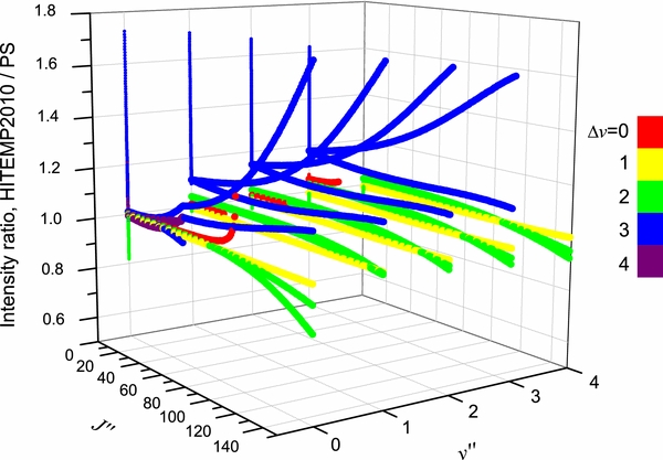
Figure 9. Comparison of line intensities of 12C16O rovibrational bands between the HITEMP2010 database and the present semi-empirical study. See text for details.
Download figure:
Standard image High-resolution image6. LINE WIDTHS AND SHIFTS
6.1. Line Widths and their Temperature Dependence
In this section, we will discuss the assembly of the complete set of air-, CO-, H2-, and CO2-broadened parameters for all the CO lines presented here. The line-shape parameters of the CO lines have been studied in dozens of publications where authors probe different spectral regions, different broadeners and different line-shape profiles. It is important to note that all of the parameters derived here assume Voigt line shape. If one seeks accuracies of the retrievals to be below the one to two percent level, this line shape is not adequate. In fact, in HITRAN2012, we have already employed the speed-dependent Voigt profile for the first overtone band. Nevertheless, we believe that for the majority of applications, the Voigt line shape will be satisfactory.
6.1.1. Air-broadened Widths
The procedure that is employed for the air-broadened parameters in HITRAN 2012 have been retained here except for the Δv = 2 bands for which the values from Malathy Devi et al. (2012b) were used. The values in HITRAN 2012 were obtained using the semi-empirical algorithm explained in the HITRAN2004 paper (Rothman et al. 2005), supplemented with high-quality experimental data, including those from Malathy Devi et al. (2012a, 2012b). The values for Δv = 3 have been used for Δv > 3 bands in this work.
6.1.2. Self-broadened Widths
Similar to air-broadened widths, the procedure that was employed for the self-broadened parameters in HITRAN 2012 have been retained here except for Δv = 2 bands for which the values from Malathy Devi et al. (2012b) were used. The values in HITRAN 2012 were developed using the semi-empirical algorithm explained in the HITRAN2004 paper (Rothman et al. 2005), supplemented with high-quality experimental data, including those from Malathy Devi et al. (2012a, 2012b). The values for Δv = 3 have been used for Δv > 3 bands in this work.
6.1.3. CO2-induced Widths
Sung & Varanasi (2005) carried out systematic measurements for the CO2-induced line widths and shifts for the 1–0, 2–0, and 3–0 bands of CO at various temperatures to determine the temperature dependence coefficients. Their values were used here. The values for Δv = 3 have been used for Δv > 3 bands. For the high-J lines whose CO2-induced widths were not measured by Sung & Varanasi (2005), the last available measured value for the highest-J line (J = 40) was adopted.
6.1.4. H2-induced Widths
There are quite a few measurements of the H2-induced broadening and shift parameters available in the literature. It is interesting to compare three studies that have carried out measurements in the 2–0 band with a wide coverage of the rotational lines (Malathy Devi et al. 2004; Régalia-Jarlot et al. 2005; Sung & Varanasi 2004b). The H2-induced broadening parameters for the 2–0 band from these three studies have been depicted in Figure 10. The results of Sung & Varanasi (2004b) and Malathy Devi et al. (2004) are in good agreement with each other, unlike the results from Régalia-Jarlot et al. (2005). Finally, the data from Malathy Devi et al. (2004) have been chosen because of the smaller uncertainties of their measurements. For the high-J values whose H2-induced widths are not measured, the available measured value for the highest-J line (J = 24) was adopted. These values were used for all other bands, neglecting vibrational dependence. This assumption seems reasonable based on the finding of Sung & Varanasi (2004b) who measured broadening in the fundamental and first and second overtone bands and found the widths to be very similar. Also, if one compares the values from the first overtone with ones measured or calculated for the pure rotational band (Dick et al. 2009; Faure et al. 2013), excellent agreement is found. All broadening values are well within 5%, whereas temperature-dependent coefficients are all within 10%. We believe this is more than satisfactory for planetary applications.

Figure 10. H2-induced line broadening for the 2–0 band of 12C16O measured by three studies: Malathy Devi et al. (2004), Sung & Varanasi (2004b), and Régalia-Jarlot et al. (2005).
Download figure:
Standard image High-resolution image6.2. Line Shifts
6.2.1. Methodology for Calculating the Semi-empirical Line Shifts
Hartmann & Boulet (2000, hereafter HB00) have successfully adopted the classic path method proposed by Neilsen & Gordon (1973) to calculate the width and shifts for HF molecules in an argon bath. Their results are in satisfactory agreement with both recent experimental measurements and the fully quantum-mechanical calculations. Most conveniently, in the Appendix, they have given a pertinent formalism that simplifies the line shift calculation. According to their theory, the line shift consists of an isotropic part and an anisotropic part which are introduced from the isotropic and anisotropic parts of the potential, respectively. The isotropic part can be further separated into symmetric and antisymmetric parts, as described below:


with the relation:


where δ(R(J)) and δ(P(J+1)) denote the line shifts for two corresponding lines R(J) and P(J+1), respectively.
Combining Equations (3) and (4), we can obtain the following relations:

It has been proven in HB00 that the symmetric part (Equation (5a)) is proportional to the difference (v'−v''), while the asymmetric part (Equation (5b)) is identical for all vibrational bands. Therefore if we choose the measurements from the first overtone (2–0) band as reference data, we could generalize the equation for both P and R branches of other rovibrational bands as follows:
where  represents the line shift for the (v' − v'') band;
  is (2–0) = 2 in this case, δ(2 − 0)symmetric (m) = 0.5 × (δ2 − 0(m) + δ2 − 0(− m)); δ(2 − 0)symmetric (m) = 0.5 × (δ2 − 0(m) − δ2 − 0(− m)); and m = −J for P branch and J + 1 for R branch transitions. Equation (6) has been adopted in our calculation of line-shift parameters for the bands where no experimental measurements of shifts are available.
6.2.2. Air-induced Shifts
The air-induced line shifts have been measured experimentally for the 1–0, 2–0, and 3–0 bands (Zou & Varanasi 2002; Malathy Devi et al. 2012b; Sung & Varanasi 2005). Among these works, the measurements of Malathy Devi et al. (2012b) for the 2–0 band have achieved an unprecedented accuracy (uncertainty <1%) using a multispectral fit procedure. To test the theoretical treatment of HB00, we took the accurate measurement of δair for the 2–0 overtone band to predict the values of δ for the 1–0 and 3–0 bands using Equation (6). The calculated results were then compared with the measurements of Zou & Varanasi (2002) and Sung & Varanasi (2005) for the 1–0 and 3–0 bands, respectively. Figure 11 shows the comparison between calculated and experimental δair for the 1–0 band. In this figure, the calculated values show a very similar pattern to the experimental ones. However, the calculated values are systematically higher than the measured values by approximately 0.0007 cm−1 atm−1 for most of the transitions. Zou & Varanasi (2002) have also calculated the air-induced shifts using the O2- and N2- induced shifts measured by Bouanich et al. (1996) assuming δair = 0.79δN2 + 0.21δO2. Their calculated results are systematically higher than their measurements by approximately 0.001 cm−1 atm−1. Since Zou & Varanasi (2002) have also reported the δair values for the 2–0 band, we compared their results with the accurate measurements of Malathy Devi et al. (2012b). It was then found that the results of Zou & Varanasi (2002) are systematically lower than those of Malathy Devi et al. (2012b) by approximately 0.0003 cm−1 atm−1. Another test was performed by calculating δair for the 1–0 band using the δair measurements of Zou & Varanasi (2002). The calculated results shown in Figure 11 are very similar to the values calculated using the data of Malathy Devi et al. (2012b). It would be interesting to see a new independent study of the 1–0 band to understand if the discrepancy is due to an oversimplified model or to issues in the actual experiment.

Figure 11. Comparison of the air-induced line shifts for the 1–0 band of 12C16O between the experimental measurements from Zou & Varanasi (2002) and the extrapolated values using Equation (6) with the 2–0 band data from Malathy Devi et al. (2012b) and with the 2–0 band from Zou & Varanasi (2002).
Download figure:
Standard image High-resolution imageFigure 12 shows the comparison between the calculated and experimental δair values of Sung & Varanasi (2005) for the 3–0 band. In this figure, the calculated values using Equation (6) agree reasonably well with the experimental values within experimental uncertainties, apart from the R(0) and R(1) lines where the experimental values are higher than the calculated values by approximately 0.0015 cm−1 atm−1. Moreover, the asymmetric features of δair between P and R branches are correctly interpreted by our calculation. It thus can be concluded that the HB00 theory should provide reasonable predictions for line-shift parameters for higher overtone bands where no experimental data are available.

Figure 12. Comparison of the air-induced line shifts for the 3–0 band of 12C16O between the experimental measurements of Sung & Varanasi (2004a) and the extrapolated values using Equation (6) with the 2–0 band data from Malathy Devi et al. (2012b).
Download figure:
Standard image High-resolution image
6.2.3. CO2-induced Shifts
Sung & Varanasi (2005) have carried out systematic measurements for the CO2-induced line widths and shifts for the 1–0, 2–0, and 3–0 bands of CO at various temperatures to determine the temperature dependence coefficients. Here, their results for line shifts have been employed to derive the corresponding values for pure rotational and higher overtone and hot bands using the HB00 theory as described above. The list containing the CO2 broadening and shifts parameters together with the associated quantum numbers has been generated and can be found in the supplementary material.
6.2.4. H2-induced shifts
7. RADIOACTIVE SPECIES
The radioactive species 14C16O, 14C17O, and 14C18O are valuable as a tracer during a nuclear explosion. Because of the large variation of the isotopic abundance of 14C in different environments, an isotopologue abundance of 100% has been assumed in generating our line lists for all three 14C-containing species, 14C16O, 14C17O, and 14C18O. The users should be aware of this detail (note that there have not been any radioactive species yet in HITRAN, and the molecules that do exist in the databases have their intensities scaled by terrestrial isotope abundances). The line list for radioactive species is given separately in the Supplementary Material.
8. CONCLUSION
The high-temperature line lists of CO are of great importance for various astrophysical, industrial, and atmospheric applications. Our updated line lists of nine isotopologues of the CO molecule is considered to be superior to previous compilations, through the use of more recent experimental data and employment of more sophisticated semi-empirical methods combined with ab initio calculations. The improved line intensities are in excellent agreement with most recent experimental data. The new ab initio calculations are found to be in good agreement with very recent experimental values.
The successful implementation of the HB00 model gave us good estimations of line shift parameters for high overtone and hot bands. The compilation of H2 and CO2 line broadening and shift parameters and their temperature dependencies in this work should be useful for the study of CO in H2- and CO2-abundant environments. In general, the updated line lists should better meet the needs of the future satellite observation of terrestrial, planetary, exoplanetary, and stellar atmospheres, high-power chemical lasers (especially the CO overtone band laser), and monitoring of automobile and plant emissions.
We offer a few recommendations for future studies to further improve the accuracy of CO line parameters.
- 1Interestingly, the fundamental band has not been measured with appropriate care of monitoring isotopic abundance in the gas cell nor with employment of sophisticated line-shape representations that include line mixing. That leaves the uncertainty for this band higher than that for the first and second overtones.
- 2More measurements for minor isotopologues in different bands are needed to construct fitted dipole moment functions for individual isotopologues and ab initio calculations carried out directly for each isotopologue are needed. This may identify potential breakdown of the Born–Oppenheimer approximation and help eliminate its effect on calculating line intensities for different isotopologues. Again determination of exact isotopic abundances in experimental gas cells is highly desirable. This can be achieved by involving a mass spectrometer, for example.
- 3Existing measurements of the fourth overtone had been carried out at very high pressure which increases the uncertainty of the measurements. With the advent of the CRDS techniques, it does not seem difficult to remeasure this band.
- 4An independent highly accurate measurement for the line intensities of an extensive set of lines in the 3–0 band is needed to resolve the disagreement between the current experimental studies.
- 5There is still room for improvement in the line position analyses which still highly rely on the solar data which does not have low uncertainty. For example, with the advent of frequency combs, it will be interesting to accurately measure the line positions of different bands for different isotopologues.
- 6The studies that employed an outdated partition function for temperature conversion of the intensities may need to be looked at with caution if one worries about fractions of percent accuracy. Also, the multi-spectrum fit in the study of Malathy Devi et al. (2012b) may need to be revisited owing to the small error in the partition function they have used. This is, however, on a fraction of a percent level.
- 7It will be beneficial to carry out independent measurements of air-induced shifts for the 1–0 band because of the systematic difference between theoretical extrapolation from the 2–0 band and experiment. Measurements in other bands are also desirable.
In general, our line list is a substantial extension and improvement over the previous efforts. It can be used by astrophysicists as is. Nevertheless, the user has to be aware that the data in these line lists will be refined when making the next official release of the HITRAN database. The line parameters for which direct high-precision measurements are available may be substituted for the semi-empirical values presented here. This will present, however, very insignificant changes, especially when one uses the line list for high-temperature applications.
For the reader's reference, the input rovibrational matrix elements and the corresponding expectation values can be found in the supplementary material (Table S1). The classic turning points on an RKR potential of CO for each vibrational level are also given (Table S2). The ab initio dipole moment function points from the present study in atomic units are listed in Table S3. The partition sums, Q(T), for all nine isotopologues with a temperature ranging from 1 to 9000 K are listed in Table S4. The line lists of 12C16O, 12C17O, 12C18O, 13C16O, 13C17O, and 13C18O in the HITRAN format can be found in supplementary files (Table S5). Corresponding CO2- and H2-broadening and shift parameters in that file are given after the traditional HITRAN 160-character record (transition) as described in a readme file. When these data become adopted for HITRAN, they will be conveniently cast into an SQL database structure that is now being developed (Hill et al. 2013). The line lists of the radioactive species 14C16O, 14C17O, and 14C18O in the HITRAN format can be found in a separate file in the supplementary materials, with 100% abundance assumed for the intensity (Table S6).
Note added in proof. After obtaining the proofs of this paper, we learned that the LEVEL8.0 version was slightly incompatible with the formalism used in Coxon & Hajigeorgiou (2004), in particular, in the handling of the variable used with the Born–Oppenheimer breakdown (BOB) functions. This resulted in a rotationally dependent deviation of the line positions in all vibrational bands. While the problem becomes appreciable only at high-J values, the line positions from this paper will have to be revised. This modification, however, does not affect the intensities or line shape parameters reported in this work. In addition, after submission of the revised version of the manuscript, we learned of the new work by Ngo et al. (2014) that reported self-broadened widths and shifts and also applied the same line-shift extrapolation procedure to self-induced shifts as we did for air-, H2- and CO2-induced values. The new study produced very similar values for self-broadened widths used by us and also confirmed the efficiency of the line-shift extrapolation algorithm used here.
We are very thankful to Professor R.J. Le Roy for providing us with potential energy functions of CO adapted to use with his program LEVEL. Dr. David Schwenke is thanked for the discussions regarding ab initio calculations. This work has been supported by NASA Planetary Atmospheres Grant NNX10AB94G. The grant from the Russian Foundation for Basic Research (12-03-00030a) to Medvedev is also thanked. The authors at LIPhy are part of Labex OSUG@2020 (ANR10 LABX56).