Probabilistic Topic Modeling for Comparative Analysis of Document Collections Probabilistic Topic Modeling for Comparative Analysis of Document Collections
ACM Trans. Knowl. Discov. Data, Vol. 14, No. 2, Article 24, Publication date: March 2020.
DOI: https://doi.org/10.1145/3369873
Probabilistic topic models, which can discover hidden patterns in documents, have been extensively studied. However, rather than learning from a single document collection, numerous real-world applications demand a comprehensive understanding of the relationships among various document sets. To address such needs, this article proposes a new model that can identify the common and discriminative aspects of multiple datasets. Specifically, our proposed method is a Bayesian approach that represents each document as a combination of common topics (shared across all document sets) and distinctive topics (distributions over words that are exclusive to a particular dataset). Through extensive experiments, we demonstrate the effectiveness of our method compared with state-of-the-art models. The proposed model can be useful for “comparative thinking” analysis in real-world document collections.
ACM Reference format:
Ting Hua, Chang-Tien Lu, Jaegul Choo, and Chandan K. Reddy. 2020. Probabilistic Topic Modeling for Comparative Analysis of Document Collections. ACM Trans. Knowl. Discov. Data 14, 2, Article 24 (March 2020), 27 pages. https://doi.org/10.1145/3369873
1 INTRODUCTION
Several domain experts suggest that “comparative thinking” is the most effective way to improve learning [49] and serves as a basis of various applications such as event summarization [45, 47], evolution analysis [13, 32], decision-making [20, 21], and interactive learning [26, 55]. Novel techniques capable of comparative thinking are therefore highly desirable in various real-world applications. The key to comparative thinking is the ability to distinguish the common and distinctive aspects between two objects [4]. In the field of data mining, topic modeling has been widely used to identify the hidden topics underlying the content [2]. In this work, we will investigate the possibility to utilize such techniques to facilitate “comparative thinking.” In other words, we would like to answer the following question: How can we simultaneously identify the common and distinctive content using topic models?
First, to achieve this goal, we will study the kinds of capabilities that are required by a desirable model. Theoretically, a model capable of “comparative thinking” should perform well in the following aspects. (1) Clearly revealing common and distinctive topics. Traditional topic modeling methods such as latent Dirichlet allocation (LDA) [2] and non-negative matrix factorization (NMF) [25] are unable to achieve good performance in discriminative learning, although running standard topic modeling methods separately on different datasets is one possible solution. However, it will generate non-comparable topics with different distributions, thus requiring additional post-processing techniques such as topic pair mapping, to further determine the common and distinctive topics. The performance of these models is unlikely to be adequate, due to the lack of clearly defined structures that can reveal common and distinctive topics. (2) Focusing on distinctive learning for content understanding. Instead of distinctive learning, most of the previous studies focused mainly on label prediction through learning class content features [23, 38, 39, 40, 43, 44]. There remains a gap in models that can identify the common and distinctive contents across datasets. (3) Learning on the entire collection level. Although there has been a vast amount of literature on mining the global and local aspects of a document corpus [7, 11, 18, 35, 52], most studies have been limited to working within one document set. The problem described here requires learning across different datasets, a far more difficult task. (4) Supporting multiple datasets. Kim et al. [19] proposed an NMF-based approach for distinctive learning named discNMF, which can handle two datasets, but it cannot easily deal with applications involving multiple datasets. As real-world tasks generally require the analysis on more than two datasets simultaneously, a general model that can be applied to arbitrary number of datasets is clearly needed.
In this article, we propose a novel approach for common and distinctive topic modeling (CDTM) on multiple datasets. CDTM is a hierarchical Bayesian model that is designed to simultaneously learn common and distinctive topics from document collections. In CDTM, several topics are global mixtures and word distributions shared by all document sets, while other topics are locally owned by each respective dataset. By word-level topic assignments, the global structures (common topics) as well as local distributions (distinctive topics) are learned within a unified framework. Through these structures, CDTM is able to discover topics characterizing a particular corpus, as well as maximally exploit the shared information across multiple corpora. This type of discriminative learning is the basis for various important applications that require “similar content comparison” and “content evolution.”
Similar content comparison. “Similar content” refers to the data belonging to the same domain (common topics), but with different emphasis or features (distinctive topics). For example, authors with different educational or cultural backgrounds are likely to have slightly different opinions on a particular subject. Figure 1 shows an example of the results obtained by applying the proposed CDTM model on news datasets published in the period of 2016 U.S. presidential election. The news articles contain word “Clinton” or “Trump” in their headlines. Figure 1(a) shows Clinton's distinctive topics, suggesting that the most significant words from her distinctive topics are related to investigations, such as “email,” “FBI,” and “security.” On the other hand, most words from Trump's distinctive topics represent issues, such as “immigration,” “border,” and “abortion.” However, as can be seen from Figure 1(b), despite facing different difficulties, the two presidential candidates share common interests such as “election,” “president,” and “voters.”

Content evolution study. The main goal of the evolution study is to understand how the overlaps and changes between old and new documents take place. More precisely, “changes” refer to fading or emerging topics (distinctive topics), and “overlaps” denote consistently discussed topics across time (common topics). Figure 2 is an illustrative example for a content evolution study. It shows how the research areas have evolved by analyzing Neural Information Processing Systems papers published from year 1987 to 2016. “Neural Networks” was the most popular term in the 1990s, followed by “SVM” and “boosting” as active research topics. “Bayesian” models such as LDA are on the rise in the later years, while “deep learning” research gains more and more attention recently. The above mentioned terms reflect the distinctive features in different time stamps. Meanwhile, several terms such as “NLP,” “converge,” and “optimization” are consistently popular over time, which belongs to the common topics of datasets across all time periods. The main contributions of this article can be summarized as follows:

- Propose a novel Bayesian model to simultaneously identify common and distinct topics among different datasets. The proposed CDTM model is the first graphical model to focus on identifying common and distinctive topics among multiple datasets, emerging from a wide range of applications.
- Explore the possibilities of discriminative learning with the variations of CDTM. Theoretically, there could be different LDA-like graphical models that can achieve discriminative learning. We explore the possibilities by designing and evaluating variations of CDTM with different structures.
- Provide guideline of usage scenarios for different models through extensive experiments. The performance of the proposed CDTM model is compared to existing state-of-the-art algorithms on real-world datasets. Our extensive quantitative and qualitative results show “when to use what method” and demonstrate the effectiveness of the proposed CDTM model.
The rest of the article is organized as follows. Section 2 reviews related work. Section 3 introduces the CDTM model and its inference process. Section 4 presents our experimental results. Section 5 concludes the article.
2 RELATED WORK
This section reviews the existing literature related to the problem studied in this article. Generally speaking, there are three main branches of research related to this work, traditional topic modeling techniques [10, 17, 25, 50], topic-class modeling [23, 38, 39, 40, 44], and methods mining global and local aspects of documents [7, 11, 18, 24, 35, 52]. Traditional topic models have been widely studied to identify the latent topics from documents. Based on these models, variations of traditional topic modeling with focus on discriminative learning can be categorized into the following two directions: topic-class modeling and global-local aspects mining. In addition to extracting topics, the topic-class modeling methods also include the concept of class, which will learn the topic distribution for different categories. On the other hand, the global–local aspect mining learns the shared and distinctive components for documents. Although these two groups of works are related to CDTM model, neither of them can handle the comparison between different datasets.
2.1 Traditional Topic Models
In general, topic models can be classified into two categories, depending on whether the approaches are based on (i) matrix decomposition such as singular value decomposition (SVD) or (ii) generative models. Probabilistic latent semantic analysis (PLSA) [10, 17] is the earliest such attempt which represents the documents as a mixture of topics and learned latent topics by performing matrix decomposition on the term-document matrix. Similarly, NMF also learned topics through matrix decomposition, applying the constraint that the decomposed matrices only included non-negative values [25]. The generative probabilistic model, LDA took a different approach by assuming a Dirichlet prior for the latent topics [2]. Theoretically, LDA-based topic modeling techniques will be able to learn coherent topics compared to matrix decomposition approaches, as they allow topic mixtures to vary in different documents [29, 50]. Many of these approaches can be used to implement the task mentioned in this article with special settings, such as LDA [2, 15] and its non-parametric variation Hierarchical Dirichlet Process [34, 51]. However, our extensive experiments conducted in this study (which are presented in Section 4) demonstrate that these approaches are unable to match the performance of CDTM, since they are not specifically designed for comparative analysis of document collections.
2.2 Topic-class Modeling
Several topic-class modeling methods have been proposed to solve the classification problem. Rosen-Zvi et al. [44] proposed the Author-Topic model, which aimed to find different topic distributions over multiple authors, where each author has a corresponding topic mixture. Based on the Author-Topic model, Lacoste-Julien et al. [23] designed discLDA to study latent topics in order to predict class labels. The main goal of the Author-Topic model is to model the interests of authors, while discLDA is to model the class properties based on content, which is also a special case of the Author-Topic model when each individual document only has one author. To bring more supervised characteristics to traditional LDA, Ramage et al. [39] proposed a variation named labeledLDA to study the mapping between latent topics and given labels. They then went on to explore the latent relationship between topics and labels with the cost of higher complexity [40]. Besides the general approaches introduced above, there are also some previous works applying the topic-class modeling to specific domains. For example, Lin et al. treated sentiment label as a special type of class: topics were dependent on sentiment distributions, while words are conditioned on the sentiment-topic pairs [27]. Rasiwasia et al. [41] studied the image classification problem by modeling each image as a word histogram and image classes as topics, and building a one-to-one mapping between topics and class labels. In summary, all of these previous works studied latent topics through class labels, and utilized the learned topical representations for label prediction. Unlike these approaches, the method we propose in this work aims to discover both the common and the different aspects of document sets.
2.3 Global-local Aspect Mining
Another branch of related works learn the structures within a single document/collection. Chemudugunta et al. [7] identified background topics and document specific topics using a variant of LDA method. Similarly, Huang et al. [18] recognized local and global aspects of documents and organized these components into a storyline via optimization. Ren et al. [42] proposed an iterative algorithm to learn phrase semantic relevance between different documents. Wang et al. [52] studied the same problem of local/global topic discovery through iterative decomposition towards events. Paul et al. [35] added an aspect variable to the LDA model so that a word may depend on a topic, an aspect, both, or neither. Ge et al. [11] proposed a method to summarize documents into chronicles according to the mapping of their underlying topics. Aspect extraction is the most widely used application of topic model based global-local aspect mining, which aims to identify descriptions for certain aspects of documents (usually product reviews). Mukherjee et al. [33] used seed words provided by users to extract aspect categories and assumed each aspect is associated with distributions over non-seed words and seed terms. Le et al. [24] proposed a supervised topic model to compare and visualize documents from multiple collections. Moghaddam et al. [31] proposed a model named Factorized LDA (FLDA), which is trained at category level to learn latent factors underlying the reviews of a category. FLDA assumes each aspect of a review should be conditioned on both the item and the reviewer. They also provided another LDA-based approach named ILDA [30], which simultaneously models aspects and their rating in order to capture the dependency between aspects and rating sentiments. However, each of these models study the patterns within one document collection, whereas our model seeks to learn the relationships among different document collections. In addition, these existing approaches work only in particular applications designed for a specific problem such as chronicles/storyline generation, rather than a general solution for document analysis.
3 PROPOSED METHOD
In this section, we introduce CDTM, a probabilistic model that aims to identify the common topics shared by multiple datasets and distinctive topics representing the unique characteristics of each dataset.
3.1 Problem Statement
CDTM is a generative probabilistic model for analyzing multiple datasets. The basic assumption in this article is that documents are represented as random mixtures over latent topics, where each topic is a distribution over words; some topics are shared by all datasets, while some other topics only belong to a specific dataset. The high-level global topics across multiple datasets are called common topics, and local distinctive topics belonging to one dataset are called specific topics. The goal of this article is to simultaneously learn both common topics and specific/distinctive topics.
Let us assume a collection of $l$ datasets, denoted by $\mathcal {C}=\lbrace \mathcal {S}_1, \mathcal {S}_2,\ldots, \mathcal {S}_l\rbrace$. In this collection, each dataset is a set of documents denoted by $\mathcal {S}=\lbrace \mathcal {D}_1, \mathcal {D}_2,\ldots, \mathcal {D}_{M_S}\rbrace$, where $M_S$ is the number of documents within the dataset $\mathcal {S}$. Each document is a sequence of $N_D$ words denoted by  . The vocabulary $\mathcal {V}$ of a collection $\mathcal {C}$ contains terms from all the datasets, and a word
  is therefore represented as a $|\mathcal {V}|$-dimensional one-hot vector. A common topic is denoted by a $K_c$-dimensional Dirichlet variable
  , and a specific topics is represented as a $K_d$-dimensional Dirichlet variable
  , where $K_c$ is the number of common topics shared by all the $l$ datasets, and $K_d$ is the number of specific topics for each dataset. The notations and variables used in this article are listed in Table 1.
| Notation | Description |
|---|---|
| $\mathcal {C}$ | a collection of multiple datasets |
| $l$ | number of datasets in collection $\mathcal {C}$ |
| $\mathcal {S}$ | a dataset of multiple documents |
| $M_S$ | number of documents in a dataset $S$ |
| $\mathcal {D}$ | a documents of multiple words |
| $N_D$ | number of words in document $\mathcal {D}$ |
| $\mathcal {V}$ | vocabulary for collection $\mathcal {C}$ |
 |
common topic mixture proportion |
 |
specific topic mixture proportion |
| $\phi _{c}$ | mixture component of common topic |
| $\phi _{d}$ | mixture component of specific topic |
| $K_c$ | number of common topics |
| $K_d$ | number of specific topics |
 |
indicator of common or specific topic choice |
| $z$ | indicator of topic choice |
| $s$ | indicator of dataset choice |
| $m$ | indicator of document choice |
| $n$ | indicator of word choice |
| $w$ | term indicator for a specific word |
| $\beta _0$/$\beta _1$ | hyperparameters for word probability matrices $\phi _{c}$/$\phi _{d}$ |
| $\alpha _0$/$\alpha _1$ | hyperparameters for topic mixtures  / / |
| $\mu$ | hyperparameter for indicator $s$ |
| $\lambda$ | hyperparameter for indicator  |
Using these definitions, the task of learning common and specific topics is modeled as the estimation for posterior distributions of Dirichlet variables  and
and  . Our proposed CDTM model is a Bayesian graphical model designed for efficiently computing these values.
3.2 The Proposed CDTM Model
A Bayesian graphical model is a type of a structured probabilistic model that utilizes a directed acyclic graph to represent the joint probability of random variables. The graphical model of CDTM model is shown in Figure 3. The circles denote latent variables; the gray ones are observable and the white ones are unobserved. The black squares represent priors, which are pre-defined parameters. The arrows indicate conditional dependencies between the variables and parameters. The plates denote the repetition of variables, which can be used to represent documents, datasets, and topics. For example, a document $\mathcal {D}$ contains $N_D$ words, which can be viewed as $N_D$ repetitions of a word variable  . Therefore, a document $\mathcal {D}$ is denoted by the plate outside of the word variable
  marked with $N_D$. Similarly, a dataset $\mathcal {S}$ with $M_S$ documents can be denoted by the plate marked with $M_S$, which is placed outside of the “document plate.”
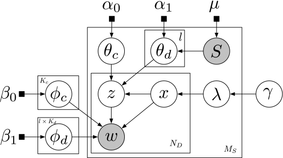

The formal generative process of the CDTM model corresponding to the graphical model shown in Figure 3 is described in Algorithm 1. The collection-level and dataset-level variables are first generated, followed by document-level variables, and finally word-level variables are generated under the constraint of upper-level variables.
Generation of collection-level and dataset-level variables. Instead of a single mixture component used in the traditional LDA, word probabilities in CDTM are parameterized by the following two kinds of topic mixture components:  (common topic) and
  (specific topic). Specifically,
  and
and  are multinomial distributions over terms that correspond to one of the common and specific topics, respectively. These are implemented as a $|\mathcal {V}|$-dimensional vector including values for all terms in vocabulary $\mathcal {V}$ of collection $\mathcal {C}$.
- Common topic mixture component
 . There are $K_c$ common topic parameters
  shared by all $l$ datasets. Therefore, in line 1 of Algorithm 1,
  is sampled $K_c$ times from a Dirichlet distribution with prior $\alpha _0$.
- Specific topic mixture component
 . Unlike common topic matrix
  , each dataset has $K_d$ different specific topics, and the entire collection has $l \times K_d$ different collection-dependent parameters
  in total. Therefore, as shown in Figure 3, there are $l \times K_d$ plates outside node
  . Similarly, in line 2 of Algorithm 1,
  is drawn $l \times K_d$ times from a Dirichlet distribution with prior $\alpha _1$.
The entire collection $\mathcal {C}$ consisting of $l$ datasets can be modeled through $l*K_d+K_c$ topics. Through the settings of topic mixture components, our proposed CDTM can model multiple datasets within a single unified framework, and simultaneously identify the common and distinctive aspects for each individual dataset.
Generation of document-level variables. In addition to collection-level mixture  and dataset-level mixture
  , we also design document-level mixtures to capture the variance for each document. Specifically, in the CDTM model, two document-level topic mixtures
  and
and  are governed by a per-document variable $\lambda$ that switches the choice between common and distinctive topics.
- Preference mixture
 . This variable is a per-document beta distribution that controls the value for per-word preference binary variable
  (will be introduced in the following paragraph).
- Common topic mixture
 . Each document has a common topic mixture
  , which is only effective when a word's preference variable
  .1
.1
- Distinctive topic mixture
 . Similarly, the document-level variable distinctive topic mixture
  only applies when a word's preference variable
  .
.
Generation of word-level variables. A word  can either be sampled from a mixture of a specific topic mixture
  , or a common topic mixture
  depending on a binary variable
  sampled from a binomial distribution
  . The generative process for words in the documents involves three stages. First, through the choice of variable
  , the CDTM model will decide whether the topic generating current word
  is a specific topic or a common topic. Afterwards, a topic indicator
  is sampled according to the document-specific mixture proportion. Finally, a word is drawn from the corresponding topic-specific term distribution.
- Choose variable
 . Per-word variable
  is chosen from a per-document multinomial distribution with prior
  .
.  indicates that the corresponding word is more likely to be generated from common topics, while
  implies the corresponding word is from a specific topic.
- Choose topic
 . After choosing
  , topic
  for each word
  is drawn from one of $K_c$ common topics if
  or from one of $K_d$ specific topics if
  .
.
- Choose term
 . Depending on the choices made for
  and
and  , word
  is generated either from a common topic-term distribution
  or sampled from specific topic-term distribution
  .
.
3.3 Inference
Although the exact inference of posterior distributions for hidden variables is generally intractable, the solution can be estimated through approximate inference algorithms, such as mean-field variational expectation [2, 15, 16], Gibbs sampling [6, 12, 36], maximum likelihood estimation [3, 9], and numerical optimization [37, 54]. Gibbs sampling is used for the inference of the proposed CDTM model, as this approach yields more accurate estimations than variational inference in LDA-like graphical models.
3.3.1 Joint Distribution. When the dataset label $s$ of the document is observed, its labeling prior $\mu$ is d-separated from the rest of the model. When $s$ is invisible, the CDTM model can be used to predict the collection label for documents. Based on Algorithm 1 and the graphical model in Figure 3, the joint distribution of the CDTM model can be represented as follows:

3.3.2 Hidden Variables. The key to this inference problem is to estimate the posterior distributions of the following hidden variables: (1) the topic assignment indicator  for words; (2) the common/distinctive preference indicator
  for words; and (3) the topic mixture proportion
  ,
,  and preference mixture proportion
  for documents. As a special case of a Markov chain Monte Carlo, Gibbs sampling iteratively samples one instance at a time, conditional on the values of the remaining given variables. We only present the result here; the detailed derivation process is omitted in order to keep the overall dicussion more clear. According to Bayes’ rule, the conditional probability of
  can be computed by dividing the joint distribution in Equation (1) by all the variables except
  . Since
  is dependent on the value of
  , the sampling of
  is discussed separately for two situations:
  or 1. When
  , which indicates that the topic
  is chosen from a common topic, the conditional probability of
  is as follows:

 , the conditional probability of
 is as shown in Equation (
3), where
$n_{dz}^v$ is the number of terms
$v$ choosing distinctive topic
$z$ in the current dataset, and
$n_{dm}^z$ is the number of words in current document
$m$ choosing distinctive topic
$z$:
is as shown in Equation (
3), where
$n_{dz}^v$ is the number of terms
$v$ choosing distinctive topic
$z$ in the current dataset, and
$n_{dm}^z$ is the number of words in current document
$m$ choosing distinctive topic
$z$:

Similar to the inference of $z$, the derivation for the posterior of  is discussed for two cases:
  or
or  . Specifically, when
  , the inference is calculated as Equation (4), where $n_m^{0}$ is the number of words choosing
  in document $m$:

 , the inference is computed using Equation (
5), where
$n_m^{1}$ is the number of words choosing
, the inference is computed using Equation (
5), where
$n_m^{1}$ is the number of words choosing
 in document
$m$:
in document
$m$:

3.3.3 Multinomial Parameters. Variables  ,
,  , $\theta _{c}$,
  and $\lambda$ are multinomial distributions with Dirichlet priors. According to Bayes rule and the definition of Dirichlet priors, these multinomial parameters can be computed from the above posteriors. For example, the common topic word distribution $\phi _{cz}$ for term $v$ and the common topic mixture $\theta _{cm}$ for document $m$ are computed as follows:
 can be calculated in a similar way:
 can be 1 or 0:
 ,
,
 , and
, and
 :
:

3.3.4 Gibbs Sampling Algorithm. The Gibbs sampling process for then CDTM model is shown in Algorithm 2. The procedure has the following five count variables: $n_{1sz}^v$ and $n_{0z}^v$ are matrices with dimension $K \times V$, $n_{1sm}^z$ has $M$ rows and $K_d$ columns, $n_{m}^x$ has dimension $M \times 2$, and $n_{0}^z$ is $K_c$ dimensional vector.
The Gibbs sampling algorithm has the following three stages: initialization, a burn-in period, and a sampling period. The determination of the optimum burn-in period duration is essential for Markov chain Monte Carlo (MCMC) approaches. In this article, we observe changes in the perplexity to check whether the Markov chain has converged. There are several strategies for using the results from Gibbs samplers. One is to read the results from one iteration (e.g., last iteration), another is to use the average of multiple samples. To obtain independent Markov chain states, here we use “sampling lag” to read results, which will leave an interval of $I$ iterations between subsequent chosen samplers.

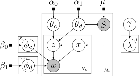
3.4 Batch CDTM Model
In this section, we will describe a batch processing variant of CDTM, called batch-CDTM model. As shown in Figure 4, control variable $\lambda$ is a dataset level parameter in the batch-CDTM model, rather than the per-document parameter in CDTM model. Using notations and terminologies similar to the ones described in Section 3.2, the joint distribution of words. topics and preference variables can be represented into the following form:

The Gibbs sampling for bath-CDTM can be performed in a similar way to that of CDTM. Therefore, here we only give the full conditional posterior for preference variable $x$:


4 EXPERIMENTS
In this section, the proposed CDTM model is evaluated with baselines using synthetic data as well as real-world datasets. We first present comparison results on synthetic data to demonstrate the superiority of the CDTM method over batch-CDTM and discNMF. And then our proposed CDTM model is also validated using different real-world datasets with various baselines. In both of these evaluations (using synthetic and real-world data), the datasets along with the comparison methods are first described, then the evaluation metrics are introduced in the following subsections, and finally the quantitative results among different approaches are presented in detail.
4.1 Evaluation on Synthetic Data
We will now describe the generation of various synthetic datasets, and then conduct analysis using these datasets to compare the performance of our proposed models and other baselines.
4.1.1 Datasets and Experimental Settings. The generation strategy for the synthetic data are as follows. Different ground truth input matrices $D_i$ for $i=1,2,\ldots,S$ can be considered as term-document matrices based on common topic matrices $W_{i,c}=[w_{i,c}^{(1)},\ldots,w_{i,c}^{(K_c)}]$ and distinctive topic matrices $W_{i,d}=[w_{i,d}^{(1)},\ldots,w_{i,d}^{(K_d)}]$. The $t$-th element ${(w_{i,c}^{(k)})_t}$ and ${(w_{i,d}^{(k)})_t}$ in the matrices can be computed as follows, where $inx(i,k)=100K_c+100(i-1)K_d+100(k-1)$:
- Label Error Rate. Label Error Rate (LER) here measures the relationship between the predicted and the ground truth labels. A lower LER value corresponds to a better performance. Given a document $m$ in dataset $\mathcal {D}$, all the models in our experiments will produce a document-level topic mixture, the topic with the largest probability value will be given the final class label $l_m$. Given the ground truth label $k_m$, the LER is computed as follows:
where $M$ is the total number of documents, $\eta (x,y)$ is equal to zero, if $x = y$, and equals to one, otherwise. In other words, $\eta (x,y)$ is the number of documents incorrectly labeled by the method.\begin{equation} LER(\mathcal {D}) = \frac{{\eta (l_m,k_m)}}{ {M}}, \end{equation}
- Similarity Score. Similarity score evaluates the similarity among the common topics of different datasets. In this article, the similarity score, which indicates how close the common topics $\Phi _{c,i}$ in dataset $\mathcal {D}_i$ is with their corresponding topics $\Phi _{c,j}$ in the other dataset $\mathcal {D}_j$, is defined as follows:
In an ideal scenario, the similarity score of common topics should be zero, since they are shared by all the datasets. Generally, a smaller value of similarity score corresponds to a better model performance.\begin{equation} f(\mathcal {D}_i,\mathcal {D}_j)_s=\sum _{z=1}^{K_c}||\phi _{c,i}^z-\phi _{c,j}^z||^2. \end{equation}
- Reconstruction Score. Reconstruction score measures the closeness of the estimated parameters produced by the models to the ground truth words. More specifically, for each document, the product of topic-term distribution and document-topic mixture will give an estimation of word occurrence probability. Reconstruction score is computed as the difference between such estimated values in document $m$ and its true words $W_m$:
Similar to similarity score and LER, a smaller value in reconstruction score means better model performance.

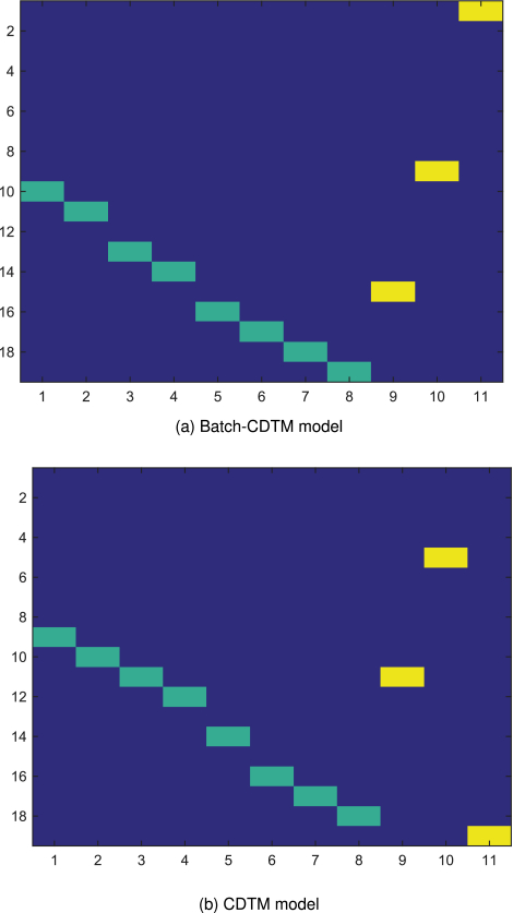
4.1.3 CDTM Vs Batch-CDTM. In this part, we compared CDTM model and its variation batch-CDTM model through illustration of result matrices and LER.
Figure 5(a) and (b) show the examples of the resulting topic-term distributions of batch-CDTM and CDTM, respecitvely. As can be seen in these figures, the performance of batch-CDTM is better than that of the CDTM. Batch-CDTM can successfully recognize all the topics and there are no overlaps between any two topics. However, CDTM makes obvious mistakes that the first common topic (topic #9) shares the same terms (terms #1,000 to #1,100) with the third distinctive topic (topic #3). To justify this observation, we run each method 20 times with random initializations and set identical initializations to both methods at each run.
In Figure 6(a) and (b), CDTM generally achieves lower error rate, compared to batch-CDTM model. As shown in Figure 6(a), both methods gain better performance with the increase of distinctive topic number $K_d$. Batch-CDTM performs poorly at the beginning, with a small value $K_d$ (equal to one). And its performance appears to be linear with respect to the values of $K_d$. CDTM model can yield relatively better performance even at the initial stage, where $K_d$ is set to be one. No obvious linear relationship between $K_d$ and performance is observed for CDTM model. However, the general trend is still similar to that of batch-CDTM: larger distinctive topic number will benefit the performance. Figure 6(b) shows the performance changes as the common topic number $K_c$ increases. Unlike the impact of distinctive topic number $K_d$, when changing common topic number $K_c$, there are no linear correlations that are observed for CDTM, nor for batch-CDTM. Both the two methods will produce lower error rates with larger common topic settings, but the curves are fluctuating.
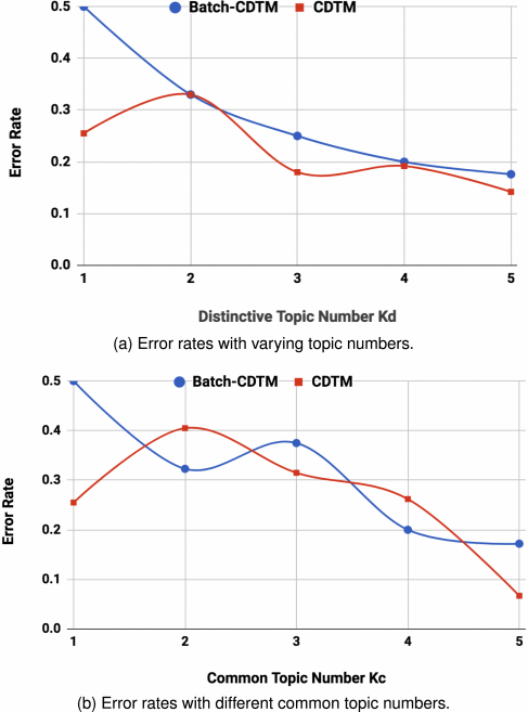
In general, Figure 5 evaluates the model performance at the dataset-level by examining the learned topics, while Figure 6 shows the results on document-level classification. As can be seen from the above the experiments, although batch-CDTM occasionally provides better topics, it is less robust than CDTM on document-level classification. Batch-CDTM can generally get better topics, as the $\lambda$ is the global parameter, and CDTM has more flexibility at the document level because its $\lambda$ parameter is assigned locally. Based on these observations, in the following document-level evaluation on real-world data, we will compare the performance of CDTM model to the other state-of-the-arts methods.
4.1.4 CDTM Vs discNMF on Multiple Datasets. As mentioned above, CDTM can be used in the analysis of multiple datasets, which is not supported by the baseline methods. In this part, we compare the performance of CDTM model with its closest baselines discNMF using the metrics of reconstruction error and similarity score on multiple synthetic datasets. Since discNMF does not support multiple datasets, we repeatedly apply it to achieve the results comparable to those of the CDTM model. However, it only works on the situation that includes $2_i (i=1,2,\ldots)$ datasets. The results studied for five datasets are presented in Table 2. Here discNMF is applied three times to get the results on five datasets. In the first application of DiscNMF, we obtained the results as combinations of dataset 1 and 2 and dataset 3 and 4. The second application of discNMF separated dataset 1 and 2, and similarly the third run of discNMF distinguished dataset 3 and 4.
| Similarity Score | Reconstruct Error | |||||
|---|---|---|---|---|---|---|
| DiscNMF | CDTM | DiscNMF | CDTM | |||
| Dataset 1 | 0.07 | 0.11 | 0 | 0 | 0.041 | 0.032 |
| Dataset 2 | 0.053 | 0.047 | ||||
| Dataset 3 | 0.09 | 0 | 0.039 | 0.022 | ||
| Dataset 4 | 0.061 | 0.056 | ||||
As can be seen from Table 2, CDTM model performs better than discNMF in both metrics, similarity score and reconstruction error. Actually, because CDTM designs a global shared data structure to model the common topics, its similarity score is zero for all datasets. DiscNMF gets a score of 0.11 in the results on combination dataset 1 and 2 and dataset 3 and 4. Smaller scores are achieved in the further separations, that discNMF gets similarity score 0.07 in topics from dataset 1 and 2, and 0.09 in the common topic similarity score for dataset 3 and 4.
4.2 Evaluation on Real-world Data
4.2.1 Datasets and Experimental Settings. To evaluate our method and other baseline comparisons, three real-world document datasets are used in our experiments: 20 News group data (20 clusters, 18,828 documents, and 43,009 keywords), Reuters dataset (65 clusters, 8,293 documents, and 18,933 keywords), and four area dataset (4 groups, 15,110 documents, 6,487 keywords). These datasets have been selected for their public availability and wide usage in topic modeling evaluations [19, 23]. Three sub-datasets are formed with different clusters, as shown in Table 3. To conduct an extensive comparison, various ratios of common and distinctive clusters are assigned to the datasets. In the Reuters data, the number of topics contained in the common cluster is the same as that in each of the exclusive clusters. while in the four area dataset, the number of common topics is larger than the number of distinctive topics.
| Common cluster | Exclusive clusters in subset 1 | Exclusive clusters in subset 2 | |
|---|---|---|---|
| Reuters | sugar | coffee | trade |
| gnp | gold | ship | |
| cpi | crude | cocoa | |
| 20 news | Alt.atheism sci.space | comp.graphics | talk.politics.guns |
| comp.sys.ibm.pc.hardware | talk.politics.mideast | ||
| comp.windows.x | talk.politics.misc | ||
| 4 area | Data Mining | Machine Learning | Database |
| Information Retrieval |
For the CDTM model, weak symmetric priors are used for all Dirichlet or Beta parameters: $\alpha _0=\alpha _1=0.1, \beta _0=\beta _1=0.001, \gamma =0.5, \mu =0.1$. It has been shown that a better performance can be obtained when the values of topic number are set closer to the real-world cases [19]. The distinctive topic number $K_d$ and common topic number $K_c$ for each dataset are therefore set as follows: (1) $K_d=3$ and $K_c=3$ in the Reuters dataset; (2) $K_d=3$ and $K_c=1$ in the 20news dataset; (3) $K_d=1$ and $K_c=2$ in the four area dataset. The Gibbs sampler is run for 400 iterations, with the first 100 iterations as burnt-in period.
4.2.2 Comparison Methods. Although there are many well studied applications on topic-class modeling [27, 41] or global-local aspect mining [7, 18], few general approaches are proposed for the purpose of discriminative learning. Since the research focus of our article is discriminative learning with topic models, the following five methods are chosen as our baseline methods, which are the most relevant approaches for our problem. LDA and NMF are most widely used state-of-the-art methods, and almost all other topic models are the variations of them. discLDA and discNMF are such variations on discriminative learning, which are the works that are closest to our proposed CDTM model. Recently, deep-learning models such as recurrent neural networks (RNN) are known to be good performers on sequence data such as text [28]. To better evaluate performance of CDTM, we also add one RNN model as the benchmark comparison method on text clustering task [46].
- LDA [2]: This is the standard topic modeling approach widely studied in the literature. We ran the LDA method on different subsets separately. For the best results, we used weak symmetric priors in our experiments: $\alpha =0.1$ and $\beta =0.001$.
- NMF [25]: This is the most popular topic modeling method based on matrix decomposition. As with the standard LDA, we applied the NMF method separately to each subset for topic discovery.
- discLDA [23]: This is a variant of LDA that is capable of discriminative modeling. There are three tunable hyperparameters $\alpha$, $\beta$, and $\pi$ in this approach, which here is set to $0.1, 0.001$, and 0.1, respectively.
- discNMF [19]: This is a discriminative topic modeling method based on NMF. To achieve best the performance, we set parameter $\alpha$ to be 100, and $\beta$ to be 10.
- LSTM [46]: Long short-term memory (LSTM) is a RNN architecture, which is widely used in sequence data such as text and speech. To perform text clustering, our implementation consists of one LSTM layer and one softmax layer, with a learning rate of 0.0001.
4.2.3 Evauation Metrics. The quality of the topic modeling results are evaluated in terms of different measures described below.
- Perplexity. Perplexity is a standard metric used to evaluate topic modeling approaches [2, 14], and is typically defined as follows:
where $M$ is the number of documents,\begin{equation} Perplexity(D) = exp\left\lbrace {\frac{{ - \sum_{m = 1}^M {\prod \nolimits _{n = 1}^N l ogP({{{\bf w}}_{mn}})} }}{{\sum_{m = 1}^M {{N_m}} }}} \right\rbrace \end{equation}
 is the word vector for document $m$ and $N_m$ is the number of words in document $m$. A lower perplexity indicates more accurate performance of the model. Here the probability of the words
  occurring in a document $m$, given its parameters, can be calculated as follows:
where $\phi _{cz_{mn}}^{w_{mn}}$ and ${\phi _{dz_{mn}}^{w_{mn}}}$ can be computed through Equations (6) and (8), while ${\theta _{cz_{mn}}^{(m)}}$ and $\theta _{dz_{mn}}^{(m)}$ can be calculated through Equations (7) and (9).\begin{equation} P(w_{mn}) = \left\lbrace \begin{array}{c}\displaystyle {\phi _{cz_{mn}}^{w_{mn}}}{\theta _{cz_{mn}}^{(m)}},\quad {\rm {if}}{\hspace{1.0pt}} {\hspace{1.0pt}} {x_{mn} = 0} \\[3pt] \displaystyle{\phi _{dz_{mn}}^{w_{mn}}}{\theta _{dz_{mn}}^{(m)}},\quad {\rm {if}}{\hspace{1.0pt}} {\hspace{1.0pt}} {x_{mn} = 1} \end{array} \right. \end{equation}
occurring in a document $m$, given its parameters, can be calculated as follows:
where $\phi _{cz_{mn}}^{w_{mn}}$ and ${\phi _{dz_{mn}}^{w_{mn}}}$ can be computed through Equations (6) and (8), while ${\theta _{cz_{mn}}^{(m)}}$ and $\theta _{dz_{mn}}^{(m)}$ can be calculated through Equations (7) and (9).\begin{equation} P(w_{mn}) = \left\lbrace \begin{array}{c}\displaystyle {\phi _{cz_{mn}}^{w_{mn}}}{\theta _{cz_{mn}}^{(m)}},\quad {\rm {if}}{\hspace{1.0pt}} {\hspace{1.0pt}} {x_{mn} = 0} \\[3pt] \displaystyle{\phi _{dz_{mn}}^{w_{mn}}}{\theta _{dz_{mn}}^{(m)}},\quad {\rm {if}}{\hspace{1.0pt}} {\hspace{1.0pt}} {x_{mn} = 1} \end{array} \right. \end{equation}
- Accuracy. Clustering accuracy (ACC) quantitatively measures the mapping relationships between resultant clusters and labeled classes [5]. A larger ACC value means better clustering performance. Given a document $m$, result label $r_m$, and ground truth label $s_m$, the cluster accuracy is computed as follows:
where $M$ is the total number of documents, $\delta (x,y)$ is a delta function that is equal to one, if $x = y$, and equals to zero, otherwise. In our evaluation, the ACC metric is used to calculate the quality of clusters, where $M$ is the total number of documents within a cluster in the ground-truth case and $\delta (x,y)$ is the number of documents correctly labeled by the methods.\begin{equation} ACC = \frac{\sum _{m=1}^{M}\delta (s_m,r_m)}{M}, \end{equation}
- Normalized Mutual Information. Normalized Mutual Information (NMI) is used to measure the quality of clusters, and is typically defined as follows:
In this article, NMI is used to evaluate clustering performance, where $c$ is the number of clusters, $n_i$ is the number of documents contained in the ground truth label $\mathcal {C}_i$, $\hat{n}_j$ is the number of documents belonging to result label $\mathcal {L}_i$, and $n_{ij}$ is the number of documents that are in the intersection between the result label $\mathcal {C}_i$ and the ground truth class $\mathcal {L}_j$. Typically, a larger $NMI$ value indicates better clustering performance.\begin{equation} NMI = \frac{\sum _{i=1}^{c}\sum _{j=1}^{c}\frac{n_{i,j}}{n}\log \frac{n \cdot n_{i,j}}{n_i\hat{n}_j}}{\sqrt {(\sum _{i=1}^{c}n_i\log \frac{n_i}{n})(\sum _{i=1}^{c}\hat{n}_j\log \frac{\hat{n}_j}{n})}}. \end{equation}
4.2.4 Parameter Sensitivity Analysis. The distinctive topic number $K_d$ is an important parameter for the discriminative learning method discLDA, discNMF, and our proposed CDTM. When keeping the total topic number $K=K_c+K_d$ fixed, Figure 7 shows the perplexity of method discLDA, discNMF, and CDTM for varying topic numbers $K_d$. The correct number of common and distinct topics here are both three. Two conclusions can be drawn from this figure.

- Minimum perplexity. Both discNMF and our proposed CDTM show minimal perplexity when $K_d$ is set to be 3, which is the correct number of discriminative topic pairs. However, there is no obvious correspondence between minimum perplexity and correct discriminative topic for discLDA.
- Sensitivity. Our proposed CDTM consistently obtains low perplexity with changes in values of $K_d$. Interestingly, another graphical model, discLDA is the second best performer in terms of variance, while matrix factorization method discNMF is very sensitive to the setting of parameter $K_d$, which increases dramatically when $K_d$ is set to be 5.
In summary, Figure 7 shows that CDTM model consistently provides results that are closer to the ground truth, discLDA is also stable with comparatively small variance, although it is hard to assign the right parameter value, while discNMF is a good performer in most cases except for the extreme values.
4.2.5 Clustering Performance. The clustering performance evaluates the quality of the resulting clusters compared to the ground-truth cluster labels. First, the cluster index for each document is computed as the most strongly associated topic index. For our proposed CDTM model, this step identifies the maximal element $\theta _{dz}$ in vector $\theta _{d}$, which can be computed similar to Equation (7). The results of discLDA are computed by jointly considering the transformation matrices and the topic mixture distribution. For the NMF and discNMF methods, this step is implemented by finding the corresponding column vector for factor matrix $H$. For LSTM, the softmax layer will generate the probability distribution of clusters, and we take the index of the maximum element in the distribution as the predicted cluster. The obtained results are then re-mapped to ground truth labels using the Hungarian algorithm [22]. Two widely adopted cluster quality measures ACC and NMI are used to evaluate the performance; these are listed in Table 4.
| Reuters | ACC | NMI | 20 news | ACC | NMI | 4 area | ACC | NMI |
|---|---|---|---|---|---|---|---|---|
| LDA | 51.327 | 0.143 | LDA | 31.141 | 0.071 | LDA | 52.864 | 0.217 |
| NMF | 55.565 | 0.221 | NMF | 34.387 | 0.125 | NMF | 44.631 | 0.147 |
| discLDA | 55.148 | 0.236 | discLDA | 33.813 | 0.122 | discLDA | 46.789 | 0.234 |
| discNMF | 54.113 | 0.228 | discNMF | 35.747 | 0.116 | discNMF | 38.136 | 0.219 |
| LSTM | 58.125 | 0.228 | LSTM | 42.243 | 0.202 | LSTM | 54.845 | 0.388 |
| CDTM | 56.815 | 0.238 | CDTM | 40.813 | 0.222 | CDTM | 55.179 | 0.391 |
| Higher values indicate better performance. |
||||||||
As shown in Table 4, we mark the best values with bold, and the second best ones with underlines. Generally, LSTM and our proposed CDTM model are best performers that outperform other existing methods (NMF, LDA, discNMF and discLDA) in all datasets for both measures ACC and NMI.
- Comparisons among different datasets. In general, the values of measure ACC and NMI for all methods will increase as the actual topic number of each cluster (6 topics for the Reuters data, 4 topics for the 20 news dataset, and 3 topics for the four area dataset) decreases. In the Reuters dataset, where the number of common and distinctive topics is the same, the five methods yield very similar results. In the 20 news dataset, as the common topic number decreases, although all methods see an increase in performance, our proposed CDTM model obtains the largest improvement. Also, in the four area dataset, where the distinctive topic number is less than the common topic number, CDTM is still the best performer, with much better ACC and NMI than other methods.
- Comparisons between CDTM and LSTM. Generally, LSTM and CDTM achieve comparable performance, that LSTM achieves better values in ACC while CDTM is the winner in terms of NMI. This is not surprising. As a deep neural network, LSTM works as a “black box.” It performs good in prediction task, but lack of explanation and understanding for output. As a result, LSTM is better in the metric of ACC, but is left behind CDTM in NMI, the metric emphasizing the quality of the clusters.
- Comparisons between CDTM and other LDA-based approaches. LDA, discLDA, and proposed CDTM model are all LDA-based approaches. CDTM is the best performer in all three datasets. discLDA is less stable, beating LDA in the datasets from Reuters and 20 news, but less well in the four area dataset. The main difference between CDTM and discLDA is that CDTM is entirely inferred through Gibbs sampling, while parameters in discLDA are estimated by a combination of Gibbs sampling and the EM algorithm. Such combination processes may result in performance instability.
- Comparisons among NMF-based approaches. Both the NMF and discNMF algorithms model topics through matrix factorization. The NMF method is slightly better than discNMF for the datasets from Reuters and four area, while discNMF performs better for the 20 news dataset. This indicates that discNMF can perform well when there is some imbalance between common and distinctive topics, but degenerates to standard NMF when common and distinctive topics have similar values. It may also suffer from the instability problem due to greater model complexity.
- Comparisons between CDTM and discNMF. In the 20 news dataset, NMF performs better than LDA, and discNMF is better than discLDA. In the four area dataset, LDA is also better than NMF, and discLDA is much better than discNMF. This indicates that LDA-based approaches can obtain good performance when there are more common topics, while NMF-based approaches can generate good results when there are more distinctive topics in the dataset.
4.3 Topic Distributions
To examine the performance, we will show the top ranked words for each topic [1, 53]. In this article, to further analyze the differences between the NMF-based and LDA-based methods, Table 5 lists the top-10 ranked words in topics learned by the discNMF model and our CDTM model. In this experiment, we utilized the four area dataset, because it is a difficult task to differentiate between these four areas due to their high content similarity between any two sub-groups. First, these four areas (data mining, information retrieval, machine learning, and database) are the closest research areas to data science, a sub-discipline of computer science. Second, in general, both “Information Retrieval” and “Data Mining” (the common topics) are on the basis on “Machine learning” (distinctive topic 1) and “Database” (distinctive topic 2). Two important observations can be made based on the results shown in Table 5.
| Distinctive Topics | |||||||
|---|---|---|---|---|---|---|---|
| Machine Learning | DataBase | ||||||
| discNMF | CDTM | discNMF | CDTM | ||||
| learning | 0.1206531 | learning | 0.019297 | database | 0.3846852 | data | 0.0280814 |
| based | 0.0459054 | based | 0.015685 | xml | 0.1141720 | query | 0.0188698 |
| model | 0.0386878 | using | 0.014255 | processing | 0.0252830 | web | 0.0171929 |
| using | 0.0337021 | data | 0.012807 | management | 0.0220824 | sql | 0.0143184 |
| reinforcement | 0.0178361 | model | 0.012477 | querying | 0.0157286 | database | 0.0121842 |
| algorithm | 0.0111599 | algorithm | 0.007233 | keyword | 0.0135791 | mining | 0.0114003 |
| classification | 0.0111518 | search | 0.007105 | sql | 0.0103898 | using | 0.0107687 |
| approach | 0.0104132 | information | 0.006738 | design | 0.0094311 | xml | 0.0099194 |
| network | 0.0103787 | clustering | 0.006738 | caching | 0.0089737 | system | 0.0094839 |
| data | 0.0088866 | classification | 0.006720 | server | 0.0088255 | efficient | 0.0088088 |
| Common Topics | |||||||
| Information Retrieval | Data Mining | ||||||
| discNMF | CDTM | discNMF | CDTM | ||||
| data | 0.0001323 | query | 0.005830 | model | 0.0035363 | web | 0.0074333 |
| based | 0.0001215 | xml | 0.004480 | game | 0.0018993 | data | 0.0055904 |
| query | 0.0001214 | web | 0.004357 | robot | 0.0016786 | mining | 0.0042388 |
| web | 0.0001213 | data | 0.004112 | planning | 0.0016436 | query | 0.0042388 |
| using | 0.0001212 | system | 0.004112 | agent | 0.0015628 | retrieval | 0.0035017 |
| mining | 0.0001211 | clustering | 0.003744 | logic | 0.0015556 | based | 0.0033788 |
| system | 0.0001206 | evaluation | 0.003621 | process | 0.0009576 | probabilistic | 0.0023959 |
| search | 0.0001205 | mining | 0.002884 | kernel | 0.0009363 | efficient | 0.0023959 |
| efficient | 0.0001203 | summary | 0.002639 | human | 0.0008836 | pattern | 0.0023959 |
| clustering | 0.0001202 | search | 0.002394 | markov | 0.0008294 | information | 0.0022730 |
- Distinctive Topic. Both discNMF and CDTM model perform well in identifying the distinctive topics “Machine learning” and “Database.” However, the results for CDTM are computed through word groups, while discNMF is more dependent on one or two of the most representative words. (1) Both methods identify the important words correctly. For example, these algorithms were able to find the most representative words in “Database,” such as “database,” “xml,” “query,” and “sql.” Also, most of the important topic words are very similar in discNMF and CDTM. For example, 7 out of the 10 top-ranked words in “Machine learning” are shared by the two methods. (2) The main difference between discNMF and CDTM is that they assign word weights within each topic differently. Compared to the CDTM model, the discNMF model seems to be more “biased” toward the most important words, with word weight dropping dramatically from the top to the bottom. For instance, in discNMF, the weights of the top ranked words (“learning” for the topic “Machine Learning” and “database” for the topic “Database”) are three times greater than the weighting awarded to the words that came in second (“based” for the topic “Machine Learning” and “xml” for the topic “Database”). This “bias” weakens the performance of discNMF as the outputs are in fact decided by a relatively small number of words, rather than the word groups used by the CDTM model.
- Common Topic. Compared to the results of the distinctive topics, both discNMF and CDTM produce less obvious results for common topics. Although this is such a difficult task that even well-trained human analyzers find it hard to distinguish a data mining article from an information Retrieval article, we can still find interesting differences in the behaviors of the discNMF and CDTM models when dealing with such tasks. (1) DiscNMF degenerates to “random guess,” while CDTM continues to give a comparatively stable performance. For discNMF, the weights of the top-ranked words in common topics are far smaller than those of distinctive topics. For instance, the weight of the top ranked word “data” for the topic “Information Retrieval” is only 0.0001323, which is more than 1,000 times smaller than that of the top-ranked word “learning” (0.1206531) for the distinctive topic “Machine leaning” and top-1 word “database” (0.3846852) in distinctive topic “Database.” Since the vocabulary size is 8,841, the weight given to the word “data,” 0.0001323, is slightly larger than $ 0.0001131$ ($1/8,841$), which suggests a “random guess,” where the weights are evenly assigned to all words. The CDTM model behaves more stably, i.e., the weights of the top ranked words in the common topics being around $1/3$ of those in distinctive words. (2) Once more, discNMF method tends to find the most representative words while CDTM considers the combined factors of the word group. DiscNMF still tries to find the most significant words, such as word “robot,” “kernel,” and “markov” in the common topic “Data Mining.” It is true that words such as “markov” are more frequently used in data mining articles than information retrieval articles, but they are only contained in a relatively small number of articles, which may therefore fail to indicate whether a article belongs to “Data Mining” or “Information Retrieval” in most cases. Similar to the case of distinctive topics, the common topics found by the CDTM model are also computed according to the combined factors from a group of words. First, the words found by the CDTM model tend to be more general than those from discNMF. For example, the topic “Data Mining” consists of exclusive words “probabilistic” and“pattern,” which are much more widely utilized in data mining articles than the words “markov” and “kernel.” Second, there are some overlaps among the top ranked words (3 out of 10) in both “Data Mining” and “Information Retrieval,” and their different weights appropriately reflect the real scenarios. For example, in the topic “Information Retrieval,” the word “query” is the most important word. Although this word also appears in the top ranked word list for “Data Mining,” it has a much smaller weight. This phenomenon reflects the true case that both “Data Mining” and “Information Retrieval” are at the intersection of “Machine Learning” and “Database,” with different emphasis on similar content.
4.4 Topic Discovery on Multiple Collections
As mentioned earlier, the proposed CDTM model is capable of handling the case of multiple datasets. This is another advantage of the CDTM model over NMF-based approaches (which can only be extended from two datasets to multi-sets with major modifications and difficulty). In this section, we discuss the interesting discoveries that can be made by applying the CDTM model to “shooting” datasets consisting of multiple document collections. This case illustrates how the CDTM model can be applied to conduct “comparative thinking” and discover interesting patterns in real-world data.
The “shooting” datasets consist of three subsets corresponding to the following three recent shooting events that occurred in the United States: “California teenager shooting,” “South Carolina Church shooting,” and “Cincinnati shooting.” The goal here is to identify the distinctive topics contained in each document set, and the common topics that are shared by all three document sets. Besides these three events, we also include some documents from other “shooting” events to generate some noise. For parameter setting, we set both common topic number $K_c$ and distinctive topic number $K_d$ to be one here. The result topic distributions are illustrated as word clouds in Figure 8.
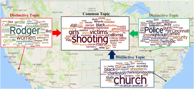
- Distinctive Topics. As the word clouds show, the top-ranked words for each event clearly reveal their characteristics. For example, in “California teenager shooting,” a teenager named “Rodger” (the biggest word) killed several victims, most of whom are “women.” Location terms are most obvious distinctive features for each of the different events, such as “cameo” for “Cincinnati shooting” and “Charleston” for “South Carolina Church shooting.” One interesting observation that can be made is that the top ranked word list includes a word labeled “YesAllWomen,” which is a prominent hashtag in Twitter. Since all our documents are news articles, this phenomenon indicates the significant influence of new emerging social media for the traditional news media. A similar conclusion can be drawn from the “South Carolina Church shooting” event, where the word “charlestonshooting” is also a hashtag from Twitter data.
- Common Topics. The common topics shared by these three events (together with the other noisy events we included) reflect the most frequently used words appearing in the “shooting” events. As can be seen from the central word cloud denoting the common topics, the two largest words, “shooting” and “victims,” are the most representative terms for all three shooting events. However, the other top ranked words also provided meaningful insights into these events. For example, the words “black,” “sex,” “girls,” and “college” are among the most important words in the list, which are consistent with the true factor that: many of the shootings are carried out by young college students, and often involving complex discrimination in gender or racism.
5 CONCLUSIONS
In this article, we proposed a novel probabilistic model called CDTM for identifying the common and distinctive topics among multiple datasets. CDTM extends a latent variable probabilistic model (e.g., LDA), by allowing the modeling of documents through choices between specific aspects of a single dataset and common aspects shared across all datasets in the collection. Extensive experiments reveal that the proposed method is not only capable of clearly identifying common and distinct topics for multiple datasets, but also capable of providing meaningful insights in the given massive data collection. The comparison against existing state-of-the-art models indicates that CDTM is more accurate than other LDA variants and more stable than the NMF-based approaches. For our future work, we plan to improve the efficiency of the proposed method, so that it can be used for real-time streaming data. In addition, we plan to build a visual analytics system [8] that can interactively visualize the common and distinctive topics. One can also naturally extend the proposed model extracting topics from short text documents by incorporating additional information [48].
ACKNOWLEDGMENTS
This work was supported in part by the U.S. National Science Foundation grants IIS-1619028, IIS-1707498, and IIS-1838730, and by the National Research Foundation of Korea (NRF) grant funded by the Korean government (MSIP) (No. NRF2019R1A2C4070420).
REFERENCES
- David M. Blei and John D. Lafferty. 2006. Dynamic topic models. In Proceedings of the International Conference on Machine Learning (ICML’06). ACM, 113–120.
- David M. Blei, Andrew Y. Ng, and Michael I. Jordan. 2003. Latent dirichlet allocation. The Journal of Machine Learning Research 3 (2003), 993–1022.
- R. Darrell Bock and Murray Aitkin. 1981. Marginal maximum likelihood estimation of item parameters: Application of an EM algorithm. In Psychometrika, Vol. 46. Springer, 443–459.
- Jordan Boyd-Graber, Yuening Hu, David Mimno, et al. 2017. Applications of topic models. Foundations and Trends® in Information Retrieval 11, 2–3, 60–62.
- Deng Cai, Xiaofei He, Xiaoyun Wu, and Jiawei Han. 2008. Non-negative matrix factorization on manifold. In Proceedings of IEEE International Conference on Data Mining (ICDM’08). IEEE, 63–72.
- George Casella and Edward I. George. 1992. Explaining the Gibbs sampler. In The American Statistician, Vol. 46. Taylor & Francis, 167–174.
- Chaitanya Chemudugunta, Padhraic Smyth, and Mark Steyvers. 2006. Modeling general and specific aspects of documents with a probabilistic topic model. In Proceedings of Neural Information Processing Systems (NIPS’06), Vol. 19. 241–248.
- Jaegul Choo, Changhyun Lee, Chandan K. Reddy, and Haesun Park. 2013. Utopian: User-driven topic modeling based on interactive nonnegative matrix factorization. In IEEE Transactions on Visualization and Computer Graphics 19, 12 (2013), 1992–2001.
- Bishop Christopher. 2007. Pattern recognition and machine learning. Springer, 93–94.
- David A. Cohn and Thomas Hofmann. 2001. The missing link-a probabilistic model of document content and hypertext connectivity. In Proceedings of the Advances in Neural Information Processing Systems (NIPS’01). 430–436.
- Tao Ge, Wenzhe Pei, Heng Ji, Sujian Li, Baobao Chang, and Zhifang Sui. 2015. Bring you to the past: Automatic generation of topically relevant event chronicles. In Proceedings of the Annual Meeting of the Association for Computational Linguistics (ACL’15). 575–585.
- Thomas L. Griffiths and Mark Steyvers. 2004. Finding scientific topics. In Proceedings of the National Academy of Sciences (PNAS’04), Vol. 101. NAS, 5228–5235.
- Bin Guo, Yi Ouyang, Cheng Zhang, Jiafan Zhang, Zhiwen Yu, Di Wu, and Yu Wang. 2017. Crowdstory: Fine-grained event storyline generation by fusion of multi-modal crowdsourced data. In Proceedings of the ACM on Interactive, Mobile, Wearable and Ubiquitous Technologies 1, 3, 55.
- Gregor Heinrich. 2008. Parameter estimation for text analysis. In University of Leipzig, Tech. Rep.
- Matthew Hoffman, Francis R. Bach, and David M. Blei. 2010. Online learning for latent dirichlet allocation. In Proceedings of the Advances in Neural Information Processing Systems (NIPS’10). 856–864.
- Matthew D. Hoffman, David M. Blei, Chong Wang, and John Paisley. 2013. Stochastic variational inference. The Journal of Machine Learning Research, Vol. 14. 1303–1347.
- Thomas Hofmann. 1999. Probabilistic latent semantic indexing. In Proceedings of the International ACM Conference on Research and Development in Information Retrieval (SIGIR’99). ACM, 50–57.
- Lifu Huang and Lian'en Huang. 2013. Optimized event storyline generation based on mixture-event-aspect model. In Proceedings of Conference on Empirical Methods on Natural Language Processing (EMNLP’13). 726–735.
- Hannah Kim, Jaegul Choo, Jingu Kim, Chandan K. Reddy, and Haesun Park. 2015. Simultaneous discovery of common and discriminative topics via joint nonnegative matrix factorization. In Proceedings of the ACM International Conference on Knowledge Discovery and Data Mining (SIGKDD’15). ACM, 567–576.
- Gang Kou, Yanqun Lu, Yi Peng, and Yong Shi. 2012. Evaluation of classification algorithms using MCDM and rank correlation. International Journal of Information Technology & Decision Making 11, 01, 197–225.
- Gang Kou, Yi Peng, and Guoxun Wang. 2014. Evaluation of clustering algorithms for financial risk analysis using MCDM methods. Information Sciences 275, 1–12.
- Harold W. Kuhn. 1955. The Hungarian method for the assignment problem. Naval Research Logistics Quarterly 2, 1 (1955), 83–97.
- Simon Lacoste-Julien, Fei Sha, and Michael I. Jordan. 2009. DiscLDA: Discriminative learning for dimensionality reduction and classification. In Proceedings of the Advances in Neural Information Processing Systems (NIPS’09). 897–904.
- Tuan Le and Leman Akoglu. 2019. ContraVis: Contrastive and visual topic modeling for comparing document collections. In Proceedings of The World Wide Web Conference. ACM, 928–938.
- Daniel D. Lee and H. Sebastian Seung. 2001. Algorithms for non-negative matrix factorization. In Proceedings of the Advances in Neural Information Processing Systems (NIPS’01). 556–562.
- Moontae Lee and David Mimno. 2017. Low-dimensional embeddings for interpretable anchor-based topic inference. In Proceedings of the 2014 Conference on Empirical Methods in Natural Language Processing (EMNLP’14). 1319–1328.
- Chenghua Lin, Yulan He, Richard Everson, and Stefan Ruger. 2011. Weakly supervised joint sentiment-topic detection from text. IEEE Transactions on Knowledge and Data engineering 24, 6, 1134–1145.
- Pengfei Liu, Xipeng Qiu, and Xuanjing Huang. 2016. Recurrent neural network for text classification with multi-task learning. In Proceedings of the International Joint Conferences on Artificial Intelligence (IJCAI’16). 2873–2879.
- David Mimno, Hanna M. Wallach, Edmund Talley, Miriam Leenders, and Andrew McCallum. 2011. Optimizing semantic coherence in topic models. In Proceedings of the Conference on Empirical Methods in Natural Language Processing (EMNLP’11). ACL, 262–272.
- Samaneh Moghaddam and Martin Ester. 2011. ILDA: Interdependent LDA model for learning latent aspects and their ratings from online product reviews. In Proceedings of the 34th International ACM SIGIR Conference on Research and Development in Information Retrieval. ACM, 665–674.
- Samaneh Moghaddam and Martin Ester. 2013. The FLDA model for aspect-based opinion mining: Addressing the cold start problem. In Proceedings of the 22nd International Conference on World Wide Web. ACM, 909–918.
- Elaheh Momeni, Shanika Karunasekera, Palash Goyal, and Kristina Lerman. 2018. Modeling evolution of topics in large-scale temporal text corpora. In Proceedings of the 12th International AAAI Conference on Web and Social Media.
- Arjun Mukherjee and Bing Liu. 2012. Aspect extraction through semi-supervised modeling. In Proceedings of the 50th Annual Meeting of the Association for Computational Linguistics: Long Papers-volume 1. Association for Computational Linguistics, 339–348.
- John Paisley, Chong Wang, David M. Blei, and Michael I. Jordan. 2015. Nested hierarchical Dirichlet processes. IEEE Transactions on Pattern Analysis and Machine Intelligence 37, 2 (2015), 56–270.
- Michael Paul and Roxana Girju. 2010. A two-dimensional topic-aspect model for discovering multi-faceted topics. In Proceedings of the Association for the Advancement of Artificial Intelligence (AAAI’10), Vol. 51. 36.
- Ian Porteous, David Newman, Alexander Ihler, Arthur Asuncion, Padhraic Smyth, and Max Welling. 2008. Fast collapsed gibbs sampling for latent dirichlet allocation. In Proceedings of the ACM International Conference on Knowledge Discovery and Data Mining (SIGKDD’08). ACM, 569–577.
- A. Kai Qin, Vicky Ling Huang, and Ponnuthurai N. Suganthan. 2009. Differential evolution algorithm with strategy adaptation for global numerical optimization. IEEE Transactions on Evolutionary Computation 13, 2 (2009), 398–417.
- Maxim Rabinovich and David M. Blei. 2014. The inverse regression topic model. In Proceedings of International Conference on Machine Learning (ICML’14). IEEE, 199–207.
- Daniel Ramage, David Hall, Ramesh Nallapati, and Christopher D. Manning. 2009. Labeled LDA: A supervised topic model for credit attribution in multi-labeled corpora. In Proceedings of Conference on Empirical Methods on Natural Language Processing (EMNLP’09). ACL, 248–256.
- Daniel Ramage, Christopher D. Manning, and Susan Dumais. 2011. Partially labeled topic models for interpretable text mining. In Proceedings of ACM International Conference on Knowledge Discovery and Data Mining (SIGKDD’11). ACM, 457–465.
- Nikhil Rasiwasia and Nuno Vasconcelos. 2013. Latent dirichlet allocation models for image classification. IEEE Transactions on Pattern Analysis and Machine Intelligence 35, 11, 2665–2679.
- Xiang Ren, Yuanhua Lv, Kuansan Wang, and Jiawei Han. 2017. Comparative document analysis for large text corpora. In Proceedings of the 10th ACM International Conference on Web Search and Data Mining. ACM, 325–334.
- Filipe Rodrigues, Mariana Lourenco, Bernardete Ribeiro, and Francisco C Pereira. 2017. Learning supervised topic models for classification and regression from crowds. IEEE Transactions on Pattern Analysis and Machine Intelligence 39, 12, 2409–2422.
- Michal Rosen-Zvi, Thomas Griffiths, Mark Steyvers, and Padhraic Smyth. 2004. The author-topic model for authors and documents. In Proceedings of the 20th Conference on Uncertainty in Artificial Intelligence (UAI’04). AUAI Press, 487–494.
- Dwijen Rudrapal, Amitava Das, and Baby Bhattacharya. 2018. A survey on automatic Twitter event summarization.Journal of Information Processing Systems 14, 1 (2018), 79–100.
- Haşim Sak, Andrew Senior, and Françoise Beaufays. 2014. Long short-term memory recurrent neural network architectures for large scale acoustic modeling. In Proceedings of the 15th Annual Conference of the International Speech Communication Association.
- Vinay Setty, Abhijit Anand, Arunav Mishra, and Avishek Anand. 2017. Modeling event importance for ranking daily news events. In Proceedings of the 10th ACM International Conference on Web Search and Data Mining. ACM, 231–240.
- Tian Shi, Kyeongpil Kang, Jaegul Choo, and Chandan K. Reddy. 2018. Short-text topic modeling via non-negative matrix factorization enriched with local word-context correlations. In Proceedings of the 2018 World Wide Web Conference. International World Wide Web Conferences Steering Committee, 1105–1114.
- Harvey F. Silver. 2010. Compare & contrast: Teaching comparative thinking to strengthen student learning. Association for Supervision & Curriculum Development, 1–2.
- Keith Stevens, Philip Kegelmeyer, David Andrzejewski, and David Buttler. 2012. Exploring topic coherence over many models and many topics. In Proceedings of the Joint Conference on Empirical Methods in Natural Language Processing (EMNLP’12) and Computational Natural Language Learning (CoNLL’12). ACL, 952–961.
- Yee W. Teh, Michael I. Jordan, Matthew J. Beal, and David M. Blei. 2005. Sharing clusters among related groups: Hierarchical Dirichlet processes. In Proceedings of the Advances in Neural Information Processing Systems (NIPS’05). 1385–1392.
- Jingjing Wang, Wenzhu Tong, Hongkun Yu, Min Li, Xiuli Ma, Haoyan Cai, Tim Hanratty, and Jiawei Han. 2015. Mining multi-aspect reflection of news events in Twitter: Discovery, linking and presentation. In Proceedings of IEEE International Conference on Data Mining (ICDM’15). IEEE, 429–438.
- Xuerui Wang and Andrew McCallum. 2006. Topics over time: A non-Markov continuous-time model of topical trends. In Proceedings of the ACM International Conference on Knowledge Discovery and Data Mining (SIGKDD’06). ACM, 424–433.
- Stephen J. Wright and Jorge Nocedal. 1999. Numerical optimization, Vol. 35. Springer Science.
- Michelle Yuan, Benjamin Van Durme, and Jordan L. Ying. 2018. Multilingual anchoring: Interactive topic modeling and alignment across languages. In Proceedings of the Advances in Neural Information Processing Systems. 8667–8677.
Footnote
- 1The value of a multinomial (binary) variable can be denoted by the index of its only non-zero element.
 denotes the zero-th element in vector $x$ is non-zero. In the rest of this article, the values of all multinomial (binary) variables are represented in this manner.
Authors’ addresses: T. Hua, Po Box 6571, Falls Church, VA, 22040; email: tingh88@vt.edu; C.-T. Lu, 7054 Haycock Road, Room 312, Falls Church, VA 22043; email: ctlu@vt.edu; J. Choo, Anam-dong 5-ga, Seongbuk-gu, Seoul 136-713, South Korea; email: jchoo@korea.ac.kr; C. Reddy, 900 N. Glebe Road, Arlington, VA 22203; email: reddy@cs.vt.edu.
Permission to make digital or hard copies of all or part of this work for personal or classroom use is granted without fee provided that copies are not made or distributed for profit or commercial advantage and that copies bear this notice and the full citation on the first page. Copyrights for components of this work owned by others than ACM must be honored. Abstracting with credit is permitted. To copy otherwise, or republish, to post on servers or to redistribute to lists, requires prior specific permission and/or a fee. Request permissions from permissions@acm.org.
©2020 Association for Computing Machinery.
1556-4681/2020/03-ART24 $15.00
DOI: https://doi.org/10.1145/3369873
Publication History: Received March 2018; revised August 2019; accepted October 2019