From Detection to Action: a Human-in-the-loop Toolkit for Anomaly Reasoning and Management
DOI: https://doi.org/10.1145/3604237.3626872
ICAIF '23: 4th ACM International Conference on AI in Finance, Brooklyn, NY, USA, November 2023
Anomalies are often indicators of malfunction or inefficiency in various systems such as manufacturing, healthcare, finance, etc. While the literature is abundant in effective detection algorithms due to this practical relevance, autonomous anomaly detection is rarely used in real-world scenarios. Especially in high-stakes applications, a human-in-the-loop is often involved in processes beyond detection such as sense-making and troubleshooting. Motivated by the financial fraud verification problem, we introduce ALARM (for Analyst-in-the-Loop Anomaly Reasoning and Management); a comprehensive end-to-end framework that supports the anomaly mining cycle from detection to action and is applicable more broadly to domains beyond finance. Besides unsupervised detection of emerging anomalies, it offers anomaly explanations and an interactive GUI for human-in-the-loop processes—visual exploration, sense-making, and ultimately action-taking via designing new detection rules—that help close “the loop” as the new rules complement rule-based supervised detection, typical of many deployed systems in practice. We demonstrate ALARM’s efficacy quantitatively and qualitatively through a series of case with fraud analysts from the financial industry.
ACM Reference Format:
Xueying Ding, Nikita Seleznev, Senthil Kumar, C. Bayan Bruss, and Leman Akoglu. 2023. From Detection to Action: a Human-in-the-loop Toolkit for Anomaly Reasoning and Management. In 4th ACM International Conference on AI in Finance (ICAIF '23), November 27--29, 2023, Brooklyn, NY, USA. ACM, New York, NY, USA 9 Pages. https://doi.org/10.1145/3604237.3626872
1 INTRODUCTION
Anomalies appear in many real-world domains, often as indicators of fault, inefficiency or malfunction in various systems such as manufacturing, environmental monitoring, surveillance, finance, computer networks, to name a few. Therefore, a large body of literature has been devoted to outlier detection algorithms [3, 5, 9] as well as open-source tools [2, 11, 20, 33].
Despite effective outlier detection algorithms, autonomous anomaly detection systems are rarely used in real world scenarios as off-the-shelf algorithms do not work well in complex situations [27]. The reason is that anomaly detection is an under-specified problem and statistical outliers are not always semantically relevant [31]. Therefore, fully automatic approaches are often impractical and the human expert (or analyst) participation and intervention are crucial. Especially in high-stakes applications, it is required, often as part of mandated policies, that the detected anomalies (credit card users flagged as malicious) go through an auditing process where the human reasons, validates and troubleshoots these anomalies.

Motivation. Anomaly explanation aims to equip the human analyst with the understanding of why the detected anomalies stand out [26]. Stand-alone explanations, however, are typically not directly utilized to improve downstream steps. There also exist various visual analytics tools specifically developed to aid detection by human perception or visual inspection to aid verification [17, 29, 30]. However, while the explanations and visualizations are expected to help the analyst gain sufficient “insight” into the anomalies, they lack explicit guidance toward decision-making and action-taking. Moreover, these detection, explanation and visualization techniques are often developed separately rather than supporting an end-to-end pipeline for human-in-the-loop anomaly mining and management for real world applications.
Application Scenario. Motivated by these gaps in the literature, we propose an end-to-end framework for anomaly mining, reasoning and management that not only equips the human-in-the-loop with anomaly explanations but also puts these explanations to use toward guiding the analyst in action-taking. Our work is driven by its applications in finance (related to bank/credit/merchant fraud and money-laundering detection and management), yet it can easily be utilized in other domains in which anomaly mining is critical.
Specifically, as shown in Fig. 1(left), we envision a deployed system where the incoming (in our case, transaction) data stream is screened through a database (i.e. ensemble) of anomaly detection rules for flagging the known type of anomalies. Rule-based detection is quite common in many real world deployed systems, thanks to the simplicity and transparency of rules (a small set of feature predicates), fast inference time, and ability to design and deploy new rules in a decentralized fashion by several experts and analysts. The overarching goal here is to quickly detect and verify new, emerging fraudulent activities and design and deploy new rule(s) that can automatically detect similar fraud in the near and far future.
Our Work. Toward this goal, we put forth the following pipeline of components. (1) Unsupervised Detection: Besides rule-based supervised detection, the data is also passed through an unsupervised detection algorithm, xStream [25, 32], for spotting emerging, unknown anomalies. (2) Explanation: We develop a built-in, model-specific explanation algorithm for xStream that estimates feature importance weights, reflective of subspaces in which the anomalies stand out the most. Importantly, the value of explanations depend on how humans put them into use [15] and to the extent that they are useful for humans in improving a downstream task [14, 28]. (3) Visual Exploration and Rule Design, with Human Interaction: To this end, as Fig. 1(right) illustrates, we leverage the explanations to present discovered anomalous patterns (i.e. clusters) to the analyst through an interactive visual interface (inset A). Anomaly clusters indicate repeating cases, of which the analyst is interested to “catch” future occurrences. The analyst can use our visual analysis tool to inspect any cluster toward verifying true vs. false positives (inset B). Notably, this is a critical step as not all statistical outliers are interesting anomalies, due to the “semantic gap” [31]. For true/semantic anomalies, we further leverage explanations to present candidate rules that best capture the verified anomalous pattern (inset C). Finally, an interactive interface allows the analyst to revise any of the candidates or design a new rule that can capture these instances (high coverage) but not others (high purity) (inset D). The newly designed rule(s) are then transferred onto the existing rule database toward flagging similar future anomalies, contributing to supervised detection and thereby closing “the loop”. In summary, this work introduces the following main contributions.
- End-to-end Pipeline for Human-in-the-loop Anomaly Discovery and Management: We develop a new end-to-end framework, called ALARM (for Analyst-in-the-Loop Anomaly Reasoning and Management), that supports (i) unsupervised emerging anomaly detection, (ii) human-in-the-loop reasoning and verification, and (iii) guided action-taking in the form of interactively designing new detection rules for future anomalies of similar nature.
- Anomaly Explanations-by-Design: We equip the unsupervised detection algorithm xStream [25, 32] with model-specific (rather than post hoc/model-agnostic) explanations (i.e. feature importances), capable of handling mixed-type data. We quantitatively evaluate the accuracy of the feature-importance based explanations by utilizing generative models that simulate mixed-type anomalies. Notably, explanations are further utilized downstream; for anomalous pattern discovery and candidate rule generation.
- Interactive Visual Toolkit for Verification and Rule Design: We create a GUI that summarizes detected anomalies in clusters (reducing one-by-one inspection overhead), allows visual inspection and exploration toward verification, and presents candidate rules for interactive, multi-objective rule design (insets A–D in Fig. 1).
- Financial Application and User Study: We employ our end-to-end framework in the financial domain wherein detecting and managing emerging fraudulent schemes in a timely fashion is critical. User studies with three real-world fraud analysts across three case studies and two datasets demonstrate the efficacy and efficiency that ALARM provides, complementing current practice.
2 Overview & Background
In our proposed ALARM pipeline, the first step is effectively detecting the emerging/novel phenomena in the incoming data stream. To this end, we employ xStream [25], which is recently extended to Apache Spark based distributed anomaly detection [32]. xStream is designed for streaming data, and can seamlessly handle feature-evolving, mixed-type data as it appears in many practical applications. Moreover, distributed detection is not only advantageous for real world domains where the data is too large to fit in a single machine, but also when data collection is inherently distributed over many servers, as is the case in the financial bank industry. Despite being an effective algorithm, xStream allows us to extend to a built-in (i.e. model-specific) explanation method.
Two downstream components of our ALARM framework, namely (1) anomaly explanation and the (2) interactive visual exploration and rule design toolkit, are developed newly as part of the current work in order to assist human analysts in the loop post detection, and thus closing the loop from detection to action.
2.1 Anomaly Detection with xStream: Review
xStream consists of three main steps, which we review briefly for the paper to be self-contained, and refer to [25] for details.
2.1.1 Step 1. Data Projection. Given mixed-type data $\mathbf {x}_i \in \mathbb {R}^D$, xStream creates a low-dim. sketch si via random projections [1, 12]:
(1)
(2)
2.1.2 Step 2. Denstiy Estimation with Half-space Chains. Anomaly detection relies on density estimation at multiple scales via a set of so-called Half-space Chains (HC), a data structure akin to multi-granular subspace histograms. Each HC has a length L, along which the (projected) feature space $\mathcal {F}_p$ is recursively halved on a randomly sampled (with replacement) feature, where fl ∈ {1, …, K} denotes the feature at level l = 1, …, L.
Given a sketch s, the goal is to efficiently identify the bin it falls into at each level. Let $\boldsymbol {\Delta }\in \mathbb {R}^K$ be the vector of initial bin widths, equal to half the range of the projected data along each dimension $f \in \mathcal {F}_p$. Let $\bar{\mathbf {z}}_l \in \mathbb {Z}^K$ denote the bin identifier of s at level l, initially all zeros. At level 1, bin-id is updated as $\bar{\mathbf {z}}_1[f_1] = \lfloor \mathbf {s}[f_1]/\boldsymbol {\Delta }[f_1] \rfloor$. At consecutive levels, it can be computed incrementally, as

(3)
Overall, xStream is an ensemble of M HCs, $\mathcal {H}= \lbrace HC^{(m)} := (\boldsymbol {\Delta }, \mathbf {f}^{(m)}, \mathcal {C}^{(m)})\rbrace _{m=1}^M$ where each HC is associated with (i) bin-width per feature $\boldsymbol {\Delta }\in \mathbb {R}^K$, (ii) sampled feature per level $\mathbf {f}^{(m)} \in \mathbb {Z}^L$, and (iii) counting data structure per level $\mathcal {C}^{(m)} = \lbrace C_l^{(m)}\rbrace _{l=1}^L$.
2.1.3 Step 3. Anomaly Scoring. To score a point for anomalousness, count of points in the bin that its sketch falls into at each level l of a HC, denoted $C_l^{(HC)}[\bar{\mathbf {z}}_l]$, is extrapolated via multiplying by 2l s.t. the counts are comparable across levels. Then, the smallest extrapolated count is considered the anomaly score, i.e.
(4)
3 ANOMALY EXPLANATION
Given the detected anomalies by xStream, we aim for model-specific explanations per anomaly, i.e., individual explanations. As detection is based on density estimates in feature subspaces, explanations aim to reflect feature importances.
3.1 Estimating Feature Importances
To estimate the weight of a feature for a high-score anomaly, we follow a simple procedure that leverages the ensemble nature of xStream. In a nutshell, it identifies the half-space chains in the ensemble that “use” the feature in binning the feature space, and (re)calculates the the anomaly score of the point only based on this set of chains. The higher it is, the more important the feature is in assigning a high score to the (anomalous) point.
Specifically, recall from Sec. 2.1.2 that $\mathbf {f}^{(m)} \in \mathbb {Z}^L$ denotes the sequence of features used in halving the feature space by chain m. Given M chains $\mathcal {H}= \lbrace HC^{(m)}\rbrace _{m=1}^M$, and a feature f to estimate its importance for a (projected) point s, we partition the chains into two groups: those that do and do not “use” f in f(m).
The definition of “use” needs care here, due to how the anomaly score of a point is estimated by a chain. Note in Eq. (4) that the level l at which the extrapolated count is the minimum provides the score; in effect, only the features up to l contribute to a point's score. Therefore, a feature is considered “used” by a chain if it is a halving feature from the top down to this scoring level only.
Let ls denote the level at which a point s is scored by a chain. A feature f is used by chain m if f ∈ f(m)[1]…f(m)[ls]. Let $\mathcal {M}_u^{(f)}$ denote the chain indices that use feature f. Then, the importance weight of f for point s is given as:
(5)
We note that several alternative importance measures did not perform well, such as the difference between scores from the chains that do and do not use f, or the drop in the anomaly score when the chains that use f are removed. The reason is multicollinearity; when chains that did not use an important feature f used correlated features instead, they continued to yield a high anomaly score.
3.2 From Projected to Original Features
Recall from Sec. 2.1.1 that xStream creates projection features k = {1…K} to sketch high-dimensional and/or mixed-type data. The chains are built using the projected features, thus, the estimated importances above are for those “compound” features.
To this end, the relations between the projected and original features can be captured as a sparse bipartite graph. Nodes k = {1…K} on one side depict the projected features with pre-computed feature importances (node weights) as described in Sec. 3.1. Nodes $F=\lbrace 1\ldots |\mathcal {F}_r \cup \mathcal {F}_c|\rbrace$ on the other side depict the original features. Note that this graph is built separately for each (anomalous) point x to be explained. Thanks to the binary hash functions, there exists an edge (k, F) only when hk(F) ≠ 0 (or for categorical F, when hk(F⊕x[F]) ≠ 0), with expected density 1/3.
To attribute importances from projection features to the original features, a simple approach could sum the importances of the projection features whose compound an original feature participates in. However, this may attribute spurious importance from a neighbor that is important due to a different feature in its compound. It would also fail to tease apart additive feature attributions [23] in the presence of multicollinearity. As an intermediate solution, we go beyond the direct neighbors and diffuse in the graph the initial projection feature weights via random walk with restart [10].
Let $\mathbf {A}\in \lbrace 0,1\rbrace ^{(K\times |\mathcal {F}_r \cup \mathcal {F}_c|)}$ denote the adjacency matrix of the bipartite graph, π = πo‖πp denote the concatenated ‘topic-sensitive’ Pagerank vector for the original and projected features, respectively, and wp be the vector of projected feature importance weights based on Eq. (5). wp is normalized to capture the fly-back probabilities, and π is initialized randomly and normalized over iterations. Then,
(6)
(7)
4 EVALUATION: ANOMALY EXPLANATION
4.1 Simulation
To assess the performance of our feature explanations, we require data containing anomalies with ground-truth feature importance weights, which (to our knowledge) does not publicly exist. To this end, we create a new simulator synthesizing anomalies in subspaces along with feature importances. A basic simulator could generate data from a predefined distribution, altering subset of features to create anomalies. However, it may produce unrealistic data. Also, consider the case where features A and B are expanded by different factors (5 times and 10 times respectively). It is not clear which feature, A or B, is more responsible for outlierness.
To overcome the above difficulties, we propose using generative models with real-world data to synthesize anomalous points and feature importances. We use the variational auto-encoder (VAE) [16] to capture complex data distributions with both real-valued and categorical features. A VAE embeds a training point x into a lower-dim. z. At training stage, the encoder minimizes the distance of a surrogate posterior qϕ(x|z) to the true pθ(z), while the decoder maximizes pθ(x|z). The likelihood of anomaly can be determined by VAE's reconstruction probability pθ(x|z), which we also use to calculate feature importances, by comparing the reconstruction probability of a feature is altered vs. not altered.
Given a dataset, we feed all the normal points into the VAE and generate m normal points $\lbrace {\bf x}_{nor}^i\rbrace _{i=1}^{m}$ with $\lbrace {\bf z}^i\rbrace _{i=1}^{m}$ hidden variables. Then, we set a threshold τ for anomalous points as:
(8)
(9)
4.2 Experiment Setup
Data: We evaluate our anomaly explanation-by-feature importances approach on three real-valued and three mixed-type datasets, which are commonly used in anomaly detection literature for tabular data. Table 1 lists the dataset names and descriptions. All data are publicly available at the UCI machine learning repository [6].1
| Name | Type | $|\mathcal {F}_c|$ | $|\mathcal {F}_r|$ |
|---|---|---|---|
| Seismic | Mixed | 4 | 11 |
| KDDCUP | Mixed | 3 | 31 |
| Hypothyroid | Mixed | 12 | 6 |
| Cardio | Real-val | 0 | 21 |
| Satellite | Real-val | 0 | 36 |
| BreastW | Real-val | 0 | 9 |
For each dataset, we remove data points with missing values and apply normal points to our simulator to generate 5000 normal points and 500 anomalies. We randomly inflate 1/3 features for each anomaly. Real-valued features are inflated to yield either global or local anomalies, as described in Sec. 4.1. Categorical features are inflated by replacing value with that of lowest probability.
| Method | Seismic | KDDCUP | Hypothyroid | Cardio | Satellite | BreastW |
| IF+SHAP (∼ 5 mins) | 0.874 ± 0.002† | 0.740 ± 0.010† | 0.810 ± 0.011 | 0.828 ± 0.005† | 0.907 ± 0.001† | 0.957 ± 0.008† |
| DIFFI (≤ 1 min) | 0.867 ± 0.013† | 0.726 ± 0.008† | 0.824 ± 0.023 | 0.823 ± 0.004† | 0.868 ± 0.005† | 0.912 ± 0.006† |
| xStream +SHAP (≥ 130 hrs) | 0.875 ± 0.006† | 0.695 ± 0.007 | 0.830 ± 0.010† | 0.847 ± 0.005† | 0.912 ± 0.003† | 0.955 ± 0.007† |
| xStream w/out proj. (≤ 1 min) | 0.873 ± 0.018† | 0.670 ± 0.010 | 0.828 ± 0.020† | 0.836 ± 0.008† | 0.910 ± 0.006† | 0.827 ± 0.005† |
| Method | Seismic | KDDCUP | Hypothyroid | Cardio | Satellite | BreastW |
| xStream w/ proj. K=15 (≤ 1 min) | 0.666 ± 0.006 * | 0.424 ± 0.006 | 0.532 ± 0.024 | 0.706 ± 0.005 † | 0.628 ± 0.006 † | 0.837 ± 0.004 † |
| xStream w/ proj. K=20 (≤ 1 min) | 0.688 ± 0.002 * | 0.444 ± 0.013 | 0.560 ± 0.008 | 0.713 ± 0.009 † | 0.652 ± 0.004 † | 0.850 ± 0.005 † |
| xStream w/ proj. K=30 (≤ 1 min) | 0.702 ± 0.003 * | 0.488 ± 0.006 * | 0.542 ± 0.016 | 0.752 ± 0.005 † | 0.675 ± 0.007 † | 0.865 ± 0.004 † |
Baselines: We evaluate our method along with two popular explanation methods: SHapley Additive exPlanations (SHAP) [23] and Depth-based Isolation Forest Feature Importance (DIFFI) [4]. SHAP is a model-free method for interpreting the output of any machine learning model. SHAP's feature importance can be computed using the predictions of both xStream as well as Isolation Forest (IF) [21] algorithm—one of the state-of-the-art anomaly detection methods for tabular data [7]. In contrast, DIFFI is a feature importance method that is specifically based on using IF as the backbone anomaly detection method.
In addition, we compare feature importances by xStream without as well as with feature projection to varying dimensions for K. We set the other hyperparameter values sufficiently large as suggested in [25] so as to obtain good detection performance.
Metrics: The main metric for evaluation is ranking based, quantifying how well we rank the features by importance; namely Normalized Discounted Cumulative Gain (NDCG) [13]. NDCG sums the relevance-weighted scores of the items in the predicted ranking to an ideal ranking. We prefer NDCG as it i) gives more weight to the top anomalous features (we apply log 2 as the base of the discount factor), and ii) can use ground-truth feature importances as the relevance score. We also measure the time for xStream and other comparison methods to acquire feature importance explanations.
4.3 Results
Table 2 displays the NDCG ranking quality w.r.t. to the synthesized ground-truth feature importances, as well as the approximate computational time required, comparing xStream (without projection) and various baseline methods. The highest NDCG scores are achieved with the combination xStream +SHAP (for detection+explanation, respectively) for almost all datasets. However, it is computationally quite demanding, taking more than 130 hours. The IF+SHAP combination provides a faster solution, delivering results in about 5 minutes, as it uses sped-up computations of SHAP [22] for tree-based methods like IF. xStream and DIFFI, two model-specific explanation methods, are even faster. xStream (w/out projection) is comparable to state-of-the-art explanation models or often the runner-up for many of the datasets. Importantly, xStream can be applied to distributed and/or streaming data, which makes it more appealing and practical for large data real-world systems, in comparison to DIFFI and IF+SHAP.
Table 3 shows the NDCG scores of xStream with different number of projections. The usage of projection diminishes xStream’s capability to detect and subsequently explain the anomalies. In other words, when projection is used there is a noticeable decrease in both AUROC and NDCG. The decline may be driven by two factors. First, when xStream is used with projection, its detection accuracy decreases which associates with lesser quality chains, making it difficult to obtain an explanation. Second, the graph propagation-based attribution is a heuristic and may not be accurate in fully capturing the direct feature effects. Nevertheless, the use of projection allows xStream to explain feature-evolving streaming data without requiring a complete retraining of the algorithm, making it more suitable for real-time applications.
Besides quantitative comparison, we also note disagreement among the explanations themselves, where different methods yield feature importances with significant variations [18]. This suggests that no explanation can be considered the definitive truth for end-users, and highlights the importance of the human in the loop: rather than blindly accepting the feature importances produced by any specific algorithm, analysts should be able to actively participate in the anomaly mining, reasoning, and management cycle.
5 FROM EXPLANATION TO ACTION: A NEW TOOLKIT FOR ANOMALY MANAGEMENT
The premise of anomaly explanations is to equip the human-in-the-loop with a deeper insight and understanding regarding the nature of the flagged anomalies. However, explanations are only as valuable as they are useful for the analysts [15], ideally in improving a downstream task with a measurable objective [14, 28].
In many real world scenarios, including our financial application domain, the analyst's main goal is to derive enough knowledge from the explanations so as to be able to prevent future anomalies of the same nature. The action toward that goal may be fixing or troubleshooting various components of a system that the analyst has access to and full control over, or involve instigating new policies regarding how the system is allowed to operate in the future.
Particularly in the financial domain, the analyst aims to deploy a new detection rule for the potential recurrences of the detected threat. Rule-based detection systems are typical of many deployed applications in the real world for several reasons. First, rules are simple; they are short and readable by humans. Second, they enable fast filtering of potentially streaming incoming data. Moreover, a database or ensemble of rules allow multiple analysts to populate the database with new rules independently, in a decentralized fashion. Therefore, our overarching approach to putting explanations into action is to build a new toolkit that facilitates designing new rules for emerging threats. The toolkit is to allow inspecting and attending not only to the anomalies as detected by an algorithm but also to those as reported by external sources (e.g. other banks, card customers, etc.).
To best support the human in the loop, we build a visual and interactive graphical user interface (GUI) for ALARM. It consists of four main building blocks, as detailed in Sec.5.1-5.4, that respectively fulfill our key design requirements: First, the anomalies need to be summarized—by grouping similar anomalies—as individually inspecting each anomaly would be too time-consuming if several hundred are flagged. Analysts are interested to capture anomalous groups or patterns (that may continue to emerge in the future), rather than one-off anomalies. Second, human analysts often prefer visually inspecting how the data generally look like and how the anomalies stand out. Their main goal in inspecting is to verify if the anomalies are truly semantically relevant or otherwise false positives. Third, analysts could benefit from automatically generated candidate rules. Data-driven rules provide a reasonable starting point that the analyst can revise, reducing the time from detection to response. Some analysts may be more novice than others and find a starting point helpful. Finally, the GUI should support fully interactive rule design that allows adding/removing feature predicates. Analysts often have years of expertise in identifying useful predicates that capture recurring attack vectors. They may also prefer some features over others for their cost-efficiency as well as for various policy reasons (justifiable, privacy, ethical, etc.).
5.1 Summary View (Sum):
Given a list of anomalies to be inspected, the summary view clusters them by similarity. Similarity is based on the feature importances as estimated by anomaly explanation (Sec. 3), rather than feature values in the original space. That is, we use $\text{sim}(\boldsymbol {\pi }_{o,i}, \boldsymbol {\pi }_{o,i^{\prime }})$ that helps group the points that stand out as anomalous in similar subspaces.

As Fig. 2 illustrates, anomalies are presented in a 2-dimensional MDS embedding space [19] for visualization, which preserves the aforementioned pairwise similarities as best as possible. The analyst can choose the number of clusters, where different symbols depict the cluster membership of the anomalies. The color of the points reflect their anomaly score from xStream. Clicking a point opens up a window that shows its feature importances in horizontal bars.
While the anomalies to be inspected could be the top k highest scoring points from xStream, ALARM also allows the analyst to import points of their own interest to inspect; e.g. (labeled) anomalies obtained via external reporting. In that case, the analyst data is passed onto xStream, which provide anomaly scores and explanations for the labeled points. Summary View displays only these labeled anomalies of interest, with explanations from xStream that are used toward clustering.
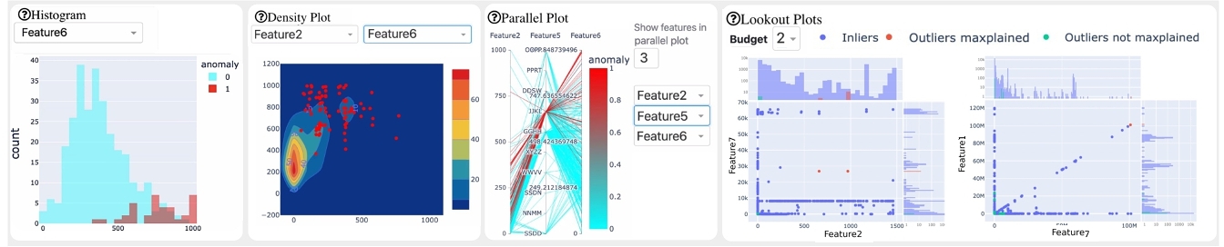
5.2 Exploration View (Expl):
Fig. 3 illustrates the tools that ALARM offers for data exploration, consisting of four main components that can aid sense-making and verification: Histogram, Density plot and Parallel plot display the comparison of anomalies vs. inliers with a single, two and multiple dimensions respectively. For all three components, the analyst is able to select which features to display. Finally, Lookout [8] presents a few scatter plots which are automatically selected feature pairs that maximally-explain (“maxplain”) the anomalies in two dimensions, i.e. wherein the anomalies stand out the most. Analyst can choose the budget interactively, adjusting the number of plots that can be used to maxplain all the anomalies.
5.3 Rule Candidates View (Cand):
Given a group of anomalies, x-PACS algorithm [24] generates concise rules, with a small set of predicates, that characterize the anomalous pattern. It estimates the univariate kernel and histogram density of the anomalous points, respectively for each numerical and nominal feature, to identify the intervals or values of significant peaks. It then combines these from selected features, where the feature intervals that define the peaks are presented as the predicates.
Fig. 4 shows a screenshot of our Rule Candidates View, which displays up to three rules that satisfy two user-specified thresholds: coverage (C) and purity (P). C is the fraction of anomalies in the group that comply with the rule, and P is the fraction of inlier points that do not pass the rule. As such, the higher both C and P are, the better, as they associate with high recall but low false alarm rates.


5.4 Rule Design Interface (RDI):
Fig. 5 illustrates a screenshot of ALARM’s interface toward facilitating the design of a new rule with high coverage and purity. The analyst can select a candidate rule to revise or design a rule from scratch by adding or deleting features, and adjusting their values. Real-valued feature predicates are adjusted by sliders that allow specifying intervals, and categorical features can be assigned a value by scrolling through a drop-down list. “Calculate Scores” button displays the coverage and purity of the latest set of predicates. Upon completion, the rule can be saved locally or in a rule database used for supervised anomaly detection.
6 FINANCIAL APPLICATION: USER STUDY
6.1 User Study Setup
Participants: We recruited three professional fraud analysts from Capital One bank to participate in our user study. The analysts had years of experience respectively, with card fraud, bank fraud, and AML (anti-money laundering) as part of their job.
Data: We conducted the user studies on two separate datasets with ground-truth anomalies. First dataset Czech is based on our simulator. From the 1999 Czech Financial Dataset2, We applied our simulator (see Sec.4.1) and simulated 1,000 normal points and 3 anomalous clusters with 20 anomalies each, based on different inflated feature subspaces. Data contains 2 numerical and 4 categorical features, as well as the inlier or anomaly cluster labels.
Second dataset Card contains a random sample of Capital One credit card transactions for a specific vendor over a period of time when they experienced a high (attempted) fraud rate. The credit card data has been anonymized with features renamed, numeric values renormalized, and categorical values hash-encoded. The dataset consists of 374 transactions, 82 of which are fraudulent or attempted fraudulent transactions. Each transaction has 3 numeric and 4 categorical features, and a label indicating whether the transaction is normal or a fraudulent one.
Procedure: We quantitatively evaluate the effectiveness and time-efficiency that ALARM provides via case studies. We also conduct an interview study and report qualitative feedback from the analysts.
Case Studies: We conducted three case studies on Czech and two case studies on Card. Each study is associated with a specific task. To avoid leakage or prior familiarity between tasks, we used a separate one of three anomalous clusters in Czech for each task. Card came equipped with an existing domain-rule from earlier investigation, which helped prevent this issue. We describe the different tasks as follows.
- Task 1: On Czech, we first ask the analyst to write a rule 1.a) using self-tools3, and then 1.b) using ALARM. We measure and compare i) quality (coverage C and purity P) of rules as well as ii) time it takes to write them (denoted time-to-rule). On Card, we skip step 1.a) as the dataset readily came with an associated domain rule, developed by earlier investigators. This study is to quantify the added benefit of ALARM vs. ad-hoc tools that analysts otherwise use.
- Task 2: On Czech, we ask the analysts to explore the automatically generated rules and improve one candidate rule using the exploration (Expl) and the rule design interface (RDI). We measure how quickly and how much they can improve the rules, in terms of average C and P. On Card, the rule to be improved is the readily available domain-rule. This study is to quantify the added benefit of Expl and RDI in improving a potentially suboptimal rule.
- Task 3: on Czech, we ask the analyst to write rules solely using Expl and RDI. We measure i) proximity of analyst-generated rules to the ground-truth, and ii) time it takes to write them (compared to avg. analyst time-to-rule via self-tools). We do not provide the analysts with any candidate rules. This study is to measure ALARM’s role in helping the analyst get to the ideal rule.
Metrics: We measure the coverage (C) and purity (P) of the rules designed as well as the duration or time-to-rule in all case studies. Interview Study: We followed the studies with a list of interview questions to which the analysts responded with short answers. The interview probed for their feedback regarding the usability and functionality of ALARM.
6.2 Case Study Results
Fig. 6 for Task 1 (ad-hoc tools vs. ALARM) demonstrates that the analysts using ALARM generally produced comparable rules to those using ad-hoc tools or to the pre-existing domain rule. On Czech, analysts have generated higher coverage rules using ad-hoc tools, only by having a disjunctive “OR” clause that treats the anomalies as two groups (while the latest version of ALARM now supports “OR” conditions). On Card, all analysts consistently produced rules with higher coverage than that of the domain-rule, sacrificing purity slightly. Since the analysts target financial fraud, they typically prioritize high coverage to avoid potentially large monetary losses from false negatives.

Furthermore, ALARM is more efficient. Different from ad-hoc tools, ALARM’s putting “the components in one place” provides an advantage. Average time-to-rule on Czech using ALARM (around 6 mins) is shorter than the time of ad-hoc tools (8 mins). On Card, all analysts were quick (also 6 mins) to produce rules comparable to the domain-rule without any training, whereas the domain rules are created with significantly longer time (“about 10-30 mins”) and require specialized domain knowledge.
Fig. 7 for Task 2 (initial-rule vs. improve-w/ALARM) shows that ALARM’s interactive exploration and rule design can assist in improving existing rules. On Czech, all analysts selected the same initial rule from among the candidates due to its simplicity (single predicate), and two of the three were able to improve to higher coverage without changing purity, within 2 mins on average. On Card, all three analysts have improved the purity of the domain-rule, with only one having to sacrifice coverage slightly, in about 6 mins on average. The improvements on Card are particularly notable, since the domain-rule for Card is already a carefully-crafted deployed rule.

On Task 3 (ground-truth vs. ALARM-w/out-Cand) we find that the ALARM-based rules explored by the analysts and the (hidden) ground-truth rule are consistent with each other, regarding their common usage of a predicate that aligns with the crucial ground-truth predicate (balance between 60000 and 75000).

As shown in Fig. 8, while one analyst built a very similar rule to the ground-truth w.r.t. coverage and purity, the others traded those in opposite directions4 by choosing different predicates besides balance. The study showcased the space of alternative rules that ALARM allowed the analysts to explore and choose from based on other hard-to-quantify metrics such as policy, ethics, and deployment cost.
6.3 Discussion on Lessons Learned
We compile a list of learned lessons based on the analysts’ interviews. Overall, the analysts found ALARM to be “valuable for exploring the data and anomalies”, “useful for comparing and contrasting”, and helpful in identifying “specific pockets of risk”.
On efficiency: Analysts agreed that ALARM is “a large time saver”, and enjoyed that it allowed them to “instantly generate rule candidates”, “quickly adjust thresholds and calculate how these adjustments affected the coverage and purity”, as well as “quickly getting a sense of where the anomalies are and how they're spread/clustered”.
On automation & interaction: While some analysts found Cand, i.e. “automatic rule mining component to be the most useful”, others perceived it as “unable to generate optimal rules” which made them “reluctant to trust” it “in favor of writing [their] own”. RDI was unanimously valued both in terms of the efficacy and efficiency it provided over manual practice: “attempt to iterate... was a massive value proposition as compared to doing this manually.”
On complexity: All analysts consistently took most advantage of the simple histogram and density plots, and some also the “string” (i.e. parallel) plot to “quickly and easily identify where anomalies were located”. However, MDS based summary viz. (esp. the axes) and the LookOut were deemed “too complex to get into”; suggesting that “individuals less familiar with ML may need robust setup instructions in order to understand and use [those]”.
Other desired functionalities: Several commented that the “ability of the user to choose their own clusters” (also split or merge existing clusters) would be “a powerful part of this tool”. While designing their rule, they liked to observe “highlights on visuals of the regions covered by rule”. One analyst suggested to add the flexibility to import additional data (e.g. last month's records from a specific vendor) while another suggested the ability to add new, analyst-crafted features. Broadly, all analysts were eager to “experiment with the tool using live data in [their] respective field” based on which they could “make more specific suggestions for improvement”.
7 CONCLUSION
We presented ALARM, a new framework for end-to-end anomaly mining, reasoning and management that supports the human analyst in the loop. It offers unsupervised detection, anomaly explanations and an interactive GUI that guides analysts toward action, i.e. new rule design. User studies with fraud analysts validate ALARM’s efficacy in finance, yet it can apply to combating emerging threats in many other domains.
REFERENCES
- Dimitris Achlioptas. 2003. Database-friendly random projections: Johnson-Lindenstrauss with binary coins. J. of Comp. and Sys. Sci. 66, 4 (2003), 671–687.
- Elke Achtert, Hans-Peter Kriegel, Lisa Reichert, Erich Schubert, Remigius Wojdanowski, and Arthur Zimek. 2010. Visual evaluation of outlier detection models. In International Conference on Database Systems for Advanced Applications. Springer, 396–399.
- Charu C. Aggarwal. 2013. Outlier Analysis. Springer. http://dx.doi.org/10.1007/978-1-4614-6396-2
- Mattia Carletti, Matteo Terzi, and Gian Antonio Susto. 2020. Interpretable Anomaly Detection with DIFFI: Depth-based Isolation Forest Feature Importance. https://doi.org/10.48550/ARXIV.2007.11117
- Varun Chandola, Arindam Banerjee, and Vipin Kumar. 2009. Anomaly detection: A survey. ACM computing surveys (CSUR) 41, 3 (2009), 1–58.
- Dheeru Dua and Casey Graff. 2017. UCI Machine Learning Repository. http://archive.ics.uci.edu/ml
- Andrew Emmott, Shubhomoy Das, Thomas Dietterich, Alan Fern, and Weng-Keen Wong. 2015. A meta-analysis of the anomaly detection problem. arXiv preprint arXiv:1503.01158 (2015).
- Nikhil Gupta, Dhivya Eswaran, Neil Shah, Leman Akoglu, and Christos Faloutsos. 2019. Beyond outlier detection: Lookout for pictorial explanation. In ECML PKDD. 122–138.
- Jiawei Han, Micheline Kamber, and Jian Pei. 2012. Outlier detection. Data mining: Concepts and Techniques (2012), 543–584.
- Taher H Haveliwala. 2002. Topic-sensitive pagerank. In Proceedings of the 11th international conference on World Wide Web. 517–526.
- Kyle Hundman, Valentino Constantinou, Christopher Laporte, Ian Colwell, and Tom Soderstrom. 2018. Detecting spacecraft anomalies using lstms and nonparametric dynamic thresholding. In Proceedings of the 24th ACM SIGKDD international conference on knowledge discovery & data mining. 387–395.
- Piotr Indyk and Rajeev Motwani. 1998. Approximate nearest neighbors: towards removing the curse of dimensionality. In STOC. 604–613.
- Kalervo Järvelin and Jaana Kekäläinen. 2017. IR Evaluation Methods for Retrieving Highly Relevant Documents. SIGIR Forum 51, 2 (aug 2017), 243–250. https://doi.org/10.1145/3130348.3130374
- Sérgio Jesus, Catarina Belém, Vladimir Balayan, João Bento, Pedro Saleiro, Pedro Bizarro, and João Gama. 2021. How can I choose an explainer? An application-grounded evaluation of post-hoc explanations. In Proceedings of the 2021 ACM Conference on Fairness, Accountability, and Transparency. 805–815.
- Harmanpreet Kaur, Harsha Nori, Samuel Jenkins, Rich Caruana, Hanna Wallach, and Jennifer Wortman Vaughan. 2020. Interpreting interpretability: understanding data scientists’ use of interpretability tools for machine learning. In Proceedings of the 2020 CHI conference on human factors in computing systems. 1–14.
- Diederik P Kingma and Max Welling. 2013. Auto-Encoding Variational Bayes. https://doi.org/10.48550/ARXIV.1312.6114
- Sungahn Ko, Isaac Cho, Shehzad Afzal, Calvin Yau, Junghoon Chae, Abish Malik, Kaethe Beck, Yun Jang, William Ribarsky, and David S Ebert. 2016. A survey on visual analysis approaches for financial data. In Computer Graphics Forum, Vol. 35. Wiley Online Library, 599–617.
- Satyapriya Krishna, Tessa Han, Alex Gu, Javin Pombra, Shahin Jabbari, Steven Wu, and Himabindu Lakkaraju. 2022. The Disagreement Problem in Explainable Machine Learning: A Practitioner's Perspective. https://doi.org/10.48550/ARXIV.2202.01602
- Joseph B Kruskal and Myron Wish. 1978. Multidimensional scaling. Number 11. Sage.
- Kwei-Herng Lai, Daochen Zha, Guanchu Wang, Junjie Xu, Yue Zhao, Devesh Kumar, Yile Chen, Purav Zumkhawaka, Minyang Wan, Diego Martinez, et al. 2021. Tods: An automated time series outlier detection system. In Proceedings of the aaai conference on artificial intelligence, Vol. 35. 16060–16062.
- Fei Tony Liu, Kai Ming Ting, and Zhi-Hua Zhou. 2008. Isolation forest. In ICDM. IEEE, 413–422.
- Scott M Lundberg, Gabriel Erion, Hugh Chen, Alex DeGrave, Jordan M Prutkin, Bala Nair, Ronit Katz, Jonathan Himmelfarb, Nisha Bansal, and Su-In Lee. 2020. From local explanations to global understanding with explainable AI for trees. Nature machine intelligence 2, 1 (2020), 56–67.
- Scott M Lundberg and Su-In Lee. 2017. A unified approach to interpreting model predictions. Advances in neural information processing systems 30 (2017).
- Meghanath Macha and Leman Akoglu. 2018. Explaining anomalies in groups with characterizing subspace rules. DAMI 32, 5 (2018), 1444–1480.
- Emaad Manzoor, Hemank Lamba, and Leman Akoglu. 2018. xStream: Outlier detection in feature-evolving data streams. In KDD. 1963–1972.
- Egawati Panjei, Le Gruenwald, Eleazar Leal, Christopher Nguyen, and Shejuti Silvia. 2022. A survey on outlier explanations. The VLDB Journal (2022), 1–32.
- Maria Riveiro, Göran Falkman, Tom Ziemke, and Thomas Kronhamn. 2009. Reasoning about anomalies: a study of the analytical process of detecting and identifying anomalous behavior in maritime traffic data. In Visual Analytics for Homeland Defense and Security, Vol. 7346. SPIE, 93–104.
- Hua Shen and Ting-Hao Huang. 2020. How useful are the machine-generated interpretations to general users? A human evaluation on guessing the incorrectly predicted labels. In Proceedings of the AAAI Conference on Human Computation and Crowdsourcing, Vol. 8. 168–172.
- Yang Shi, Yuyin Liu, Hanghang Tong, Jingrui He, Gang Yan, and Nan Cao. 2020. Visual analytics of anomalous user behaviors: A survey. IEEE Transactions on Big Data (2020).
- Hadi Shiravi, Ali Shiravi, and Ali A Ghorbani. 2011. A survey of visualization systems for network security. IEEE Transactions on visualization and computer graphics 18, 8 (2011), 1313–1329.
- Robin Sommer and Vern Paxson. 2010. Outside the closed world: On using machine learning for network intrusion detection. In 2010 IEEE symposium on security and privacy. IEEE, 305–316.
- Sean Zhang, Varun Ursekar, and Leman Akoglu. 2022. Sparx: Distributed Outlier Detection at Scale. In KDD. 4530–4540.
- Yue Zhao, Zain Nasrullah, and Zheng Li. 2019. PyOD: A Python Toolbox for Scalable Outlier Detection. Journal of Machine Learning Research 20, 96 (2019), 1–7. http://jmlr.org/papers/v20/19-011.html
FOOTNOTE
1Also downloadable from http://odds.cs.stonybrook.edu
2 https://www.kaggle.com/datasets/mariammariamr/1999-czech-financial-dataset
3Our analysts across various fraud domains used various ad-hoc tools such as Excel, pivot tables, SQL, etc. In contrast, ALARM proved to be a unified tool for all.
4As automatic candidates were not allowed in Task 3, Analyst2, who had found them most useful previously, started with a large trade-off and chose to focus on coverage.

This work is licensed under a Creative Commons Attribution-NonCommercial International 4.0 License.
ICAIF '23, November 27–29, 2023, Brooklyn, NY, USA
© 2023 Copyright held by the owner/author(s).
ACM ISBN 979-8-4007-0240-2/23/11.
DOI: https://doi.org/10.1145/3604237.3626872