Abstract
How to improve the classification accuracy is a key issue in four-class motor imagery-based brain-computer interface (MI-BCI) systems. In this paper, a method based on phase synchronization analysis and common spatial pattern (CSP) algorithm is proposed. The proposed method embodies the idea of the inverted binary tree, which transforms the multi-class problem into several binary problems. First, the phase locking value (PLV) is calculated as a feature of phase synchronization, then the calculated correlation coefficients of the phase synchronization features are used to construct two pairs of class. Subsequently, we use CSP to extract the features of each class pair and use the linear discriminant analysis (LDA) to classify the test samples and obtain coarse classification results. Finally, the two classes obtained from the coarse classification form a new class pair. We use CSP and LDA to classify the test samples and get the fine classification results. The performance of method is evaluated on BCI Competition IV dataset IIa. The average kappa coefficient of our method is ranked third among the experimental results of the first five contestants. In addition, the classification performance of several subjects is significantly improved. These results show this method is effective for multi-class motor imagery classification.
You have full access to this open access chapter, Download conference paper PDF
Keywords
- Electroencephalography
- Motor imagery
- Phase synchronization
- Common spatial pattern
- Linear discriminant analysis
1 Introduction
Brain-computer interface (BCI) is a direct communication and control channel between the human brain and a computer or other electronic device, through which people can express ideas or manipulate devices directly through the brain without using language or action [1]. It can effectively improve the ability of patients with severe disabilities to communicate with the outside or control external environment [2]. The BCI research team often use EEG to measure the biological brain signal [3]. Brain wave is a method of recording brain activity using the electrophysiological index [4]. It records the wave changes during brain activity and is the overall reflection of the electrophysiological activity of the brain cells in the cerebral cortex or scalp surface [5]. When a certain region of the cerebral cortex is activated by the senses, action instructions or motion imagination and other stimuli, the region’s metabolism and blood stream increase, at the same time, the information is processing. These can lead to the amplitude reduction or block of the corresponding band of the EEG signal. This kind of electrophysiological phenomenon is called ‘event-related desynchronization’ or ERD. The brain exhibits a significant increase in electrical activity at quiescent conditions, which is called ‘event-related synchronization’ or ERS [3]. The theoretical basis of motion imagination lies in ERS and ERD.
Motor imagery (MI) refers to a psychological process that there are individual rehearsal and simulation of the given actions but no obvious physical activity [6]. Relevant studies have shown that the neuronal activity of the primary sensorimotor areas generated by motor imagery is similar to the neuron activities of primary sensorimotor areas generated by actual motion [7, 8]. The biggest advantage of the motor imagery-based brain-computer interface (MI-BCI) system is that the EEG signal is generated by imagination without relying on any sensory stimulation. Therefore, many BCI teams based on motion imagination are devoted to the study of EEG feature extraction and classification algorithms, especially for the classification of the four-class motor imagery. Peng et al. [9] proposed a discriminative extremum learning machine with a supervised sparse preservation (SPELM) model, which is effective in multi-class classification tasks and regression tasks. Gouy-Pailler et al. [10] proposed maximum likelihood framework to improve the classification recognition rate of multi-class BCI paradigms, bridging the gap between the common spatial model (CSP) and blind source separation (BSS) of non-stationary sources. The average kappa value is 0.50. Nicolas-Alonso et al. [11] used a method for classifying four-level motion imaging tasks by combining adaptive processing and semi-supervised learning. The kappa coefficient is 0.70. He et al. [12] constructed a common Bayesian network by selecting relevant channels using nodes with common and different edges, and then classified them with SVM. The average kappa coefficient reaches 0.66.
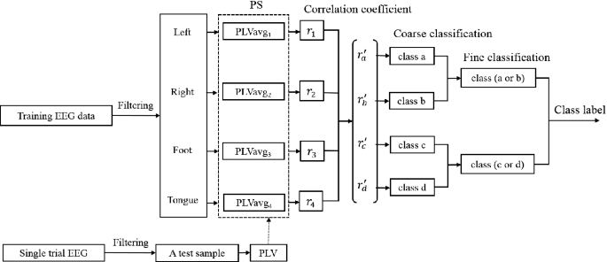
The main purpose of this paper is to propose an inverted binary tree classification method which combines phase synchronization analysis and common spatial pattern (CSP). This method can improve the classification accuracy of multi-class motor imagery EEG. We assess this method on the data set IIa which contains four different motor imagery tasks. First, the phase locking value (PLV) is calculated as a feature of phase synchronization, then the calculated correlation coefficients of the phase synchronization features are used to construct two pairs of class. Then, we use CSP to extract the features of each class pair and use the linear discriminant analysis (LDA) to classify the test samples and obtain coarse classification results. Finally, the two classes obtained from the coarse classification form a new class pair. CSP and LDA are still used to classify the test samples and get the fine classification results.
This paper is organized as follows. Section 2 describes the BCI Competition IV dataset IIa. In Sect. 3, processing methods and all steps of the proposed method are described in detail. Experimental results are presented in Sect. 4. Finally, Sect. 5 concludes the paper.
2 Data Acquisition
Our experiment uses the dataset IIa, which is available from the 4\(^{th}\) International BCI Competition (BCI-IV) and is provided by the Graz Technical University. Detailed description about dataset IIa can be downloaded from the website (http://www.bbci.de/competition/iv/#datasets). It consists of EEG data from nine subjects (named as A01, A02, A03, A04, A05, A06, A07, A08, A09, respectively). The cue-based BCI paradigm comprises four classes of motor imagery EEG measurements, namely left hand (class 1), right hand (class 2), feet (class 3), and tongue (class 4). Two sessions are recorded for each subject on different days, one for training and the other for evaluation. Each session is composed of 6 runs separated by short breaks. Each run consists of 48 trials (each class appears 12 times), yielding 288 trials per session. The timing scheme of one trial is illustrated in Fig. 1.

Timing scheme of the paradigm for recording dataset IIa.
The subjects sit in the comfortable armchair in front of the computer screen. A cue arrow indicates to perform the desired motor imagery task. The experimental data are recorded with 22 Ag/AgCl electrodes (3.5 cm inter-electrode distance) and 3 monopolar EOG channels. The signals are sampled with 250 Hz and bandpass-filtered between 0.5 Hz and 100 Hz.
The competition requires participants to provide a continuous classification output for each sample in the form of class labels that could be ‘1’, ‘2’, ‘3’ or ‘4’. The winner is the algorithm with the largest kappa value.
3 Methods
3.1 Data Preprocessing
In this work, the original signals derived from the BCI-IV are intercepted into single-trial data. The above-described data is then filtered between 8 Hz and 30 Hz with a third-order Butterworth bandpass filter. This band-pass frequency range is used because it covers both mu (8–12Hz) and beta (18–25Hz) rhythms. It can be seen from the timing scheme of one trial that the real motor imagery is starting at 3 s. Therefore, for the following feature extraction and classification, the 3 s data from 3 s to 6 s are intercepted from the filter data. The length of data for each sample is 750 data points.
3.2 Phase Synchronization Analysis
Phase synchronization analysis is based on the interrelation of the phase and the EEG with synchronization angle [13]. It can retain the phase components of EEG signals and inhibit the impact of amplitude.
For a continuous time signal x(t) recoded from channel x, its complex analysis signal by Hilbert transform can be defined as:
where \(A_x(t)\) and \(\varPhi _x(t)\) are the instantaneous amplitude and instantaneous phases of signals x(t), respectively. \(\tilde{x}(t)\) is the Hilbert transform of \(\varPhi _x(t)\). Analogously, y(t) represent the signal recoded from channel y, we define \(Z_y(t)=A_y(t)e^{i\varPhi _y(t)}\) for signal y(t).
There are many methods to measure synchronization. PLV is an important measure of phase synchronization when studying biosignals, especially electrical brain activities [14], and is defined as:
where \(<.>\) means the averaging operator of a continues time t. \(\varPhi _x(t)\) and \(\varPhi _y(t)\) are the instantaneous phases of the analytical signals \(Z_x(t)\) and \(Z_y(t)\), respectively.
Every two channels can be used to build different channel pairs. Dataset IIa has 22 channels. We calculate PLV of all channel pairs. And a symmetric matrix \(\mathbf {K}\) with dimension \(c\times c\) can be obtained. The matrix \(\mathbf {K}\) is given as:
The average PLV is defined as:
where \(N_i\) is the number of samples belonging to class i. i denotes either class 1, 2, 3 or 4.
3.3 Correlation Coefficients of Phase Synchronization Features
The correlation coefficient calculation formula is defined as:
where \(\mathbf {A}\) represents a symmetric matrix composed of the PLV value of a test sample, and \(\mathbf {B}\) represents a symmetric matrix composed of the average PLV values of the training samples of each class. \(\mathbf {\overline{A}}\) is equal to \(mean(\mathbf {A})\) and \(\mathbf {\overline{B}}\) is equal to \(mean(\mathbf {B})\). m and n denote the row and column of the matrix \(\mathbf {A}\) and \(\mathbf {B}\), respectively. In this paper, as introduced in the Sect. 3.2, m and n are the same, which are equal to the number of EEG signal channels. The dataset IIa contains four classes of motor imagery EEG data, so each test sample will form four correlation coefficients. Thereby, a column vector R can be obtained:
where \(r_1\), \(r_2\), \(r_3\) and \(r_4\) denote the correlation coefficient.
Then we can get a new column vector \(\mathbf {c}\) from \(\mathbf {r}\), and \(\mathbf {c}\) can be expressed as:
\(r_{a}^{'}=abs(r_i-mean(R))\). Analogously, \(r_{b}^{'}\), \(r_{c}^{'}\) and \(r_{d}^{'}\) have the same meaning.
3.4 Coarse Classification and Fine Classification
The proposed method mainly consists of two aspects: coarse classification of test samples based on phase synchronization feature correlation coefficients and fine classification of test samples based on coarse classification.
For coarse classification, we use the two classes of EEG data set corresponding to the first two correlation coefficients in \(\mathbf {c}\) as the training samples for CSP feature extraction, and use LDA to classify the test samples. The test samples are classified into one of the two classes. The same operation on the last two correlation coefficients and the result are classified into the other classes.
For fine classification, with the result of coarse classification, we can get a new pair of class and then make fine classification of the test sample with the CSP and LDA to acquire final classification result.
3.5 Summary of the Proposed Method
Figure 2 shows a detailed flow chart of the proposed method. The method includes several stages: signal preprocessing with a third-order Butterworth bandpass filter, use phase synchronization analysis to measure the relationship between two different channels, calculate the correlation coefficients of phase synchronization features, coarse classification and fine classification (CSP is used to extract features and LDA is employed to classify a test sample).
Flow chart of the proposed method.
4 Experiments
4.1 Phase Synchronization Features
Dataset IIa uses 22 electrodes for data acquisition, including four-class motor imagery tasks. For training data sets, we calculate the PLV of all channel pairs and get the average PLV of each class. Each class includes 72 samples. Taking the subject A03 as an example, the average PLV matrices of each class is shown in Fig. 3. The matrix contains the interaction between the channel pairs and the instantaneous phase between the channels. The closer the chroma to 1, the more synchronized the EEG signals of the two channels. It can be seen from the figure that the average PLV feature obtained from various classes of EEG training sample is different, which can be used to classify the EEG signal.

The average PLV matrices of each class on training dataset.
4.2 Topography of Optimal Spatial Filter
The proposed algorithm utilizes one versus one CSP algorithm to find the appropriate spatial filter which can maximize the difference between the two classes. That is, the variance of one class is maximized while the variance of the other class is minimized. In this paper, the optimal spatial filter is constructed by selecting 8 optimal projection directions (the first 4 rows and the last 4 rows). The projection direction of the spatial filter can be visualized by brain topography. Figure 4 shows the first and the last columns of the CSP filter, which corresponds to the maximum and the minimum eigenvalues of subject A03. The brain topography reflects the neural activity of the brain intuitively. After optimizing the pairing, there are significant differences in the EEG data of the two classes of motor imagery in each class pair. From the figure, we can also see the features of ERD/ERS produced by four kinds of motor imagery, which are effective for the classification of EEG data.

Topographic map of the first and last eigenvector of CSP filters for classifying different single-trial test samples, and 22 electrode locations. The results for subject A03 are shown.

(a) Feature subspace mapping of class 4 and class 2, coarse classification. (b) Feature subspace mapping of class 3 and class 1, coarse classification. (c) Feature subspace mapping of class 2 and class 3, fine classification.
4.3 CSP Features Subspace Mapping
The CSP algorithm is used to calculate the eigenvector, and each sample produces an 8-dimensional eigenvector, i.e. \(\mathbf {f}=[f_1,f_2,\cdots ,f_8]\). Take the subject A03 as an example, we select two spatial features from the optimized CSP features as the research object. The final result can carry out by optimizing group for three times only and constructing three spatial filters. Figure 5 shows the feature subspace mapping between the optimized combinatorial classes. The optimized combination is as follows: first, Fig. 5(a) and (b) make coarse classification of the combination of class 2 and class 4, and the combination of class 3 and class 1. Then, Fig. 5(c) obtain new optimization group and make fine classification of class 2 and class 1, which is eventually divided into class 2.
4.4 Classification Results
After coarse classification and fine classification, the predicted label by experiment and the real label are compared to determine the coarse classification and fine classification accuracy. Table 1 shows the classification accuracy of method proposed in this paper in handling the dataset IIa.
Table 1 shows that the nine subjects have a coarse classification whose accuracy range from 62.2% (A05) to 96.9% (A01) with an average of 81.75%. The fine classification accuracy range from 37.2% (A05) to 79.2% (A09) with an average of 62.66%. Obviously, the accuracy of coarse classification will affect the fine classification accuracy to a certain extent. The coarse classification accuracy of some subjects is about 90%, such as A01, A03, A07, A08, A09, and the corresponding fine classification accuracy is higher than other subjects.
We also calculate the confusion matrix of the four subjects, as shown in Fig. 6. It can be seen from the figure that the accuracy rate of right-hand motor imagery of subjects A03 is 100%, which is higher than all the other subjects. However, the accuracy of his feet motor imagery is the lowest. It can be inferred that the subject may be more concentrated during the right-hand motor imagery. In addition, the diagonal elements of the confusion matrix are always the largest, which indicates that the proposed method is applicable to the classification of multi-class motor imagery tasks.

Confusion matrices of four different subjects.
In the dataset IIa BCI competition IV, the winner is the method with the largest kappa coefficient. In order to make a fair comparison with the outcome of the competition, we use the same standard, that is, the kappa value obtained according to [15]. Table 2 presents the kappa values obtained from the proposed method in this paper and the best five competitors. A description of the results and the methods are provided on the website (http://www.bbci.de/competition/iv/results/index.html).
Table 2 shows that our approach produces quite good results in multi-class and multi-channel EEG identification, with the average kappa coefficient accounting for the third of the six different approaches, slightly below the first contestant (down 0.07) [16] and the second contestant (down 0.02) [17]. However, our algorithm has a significant advantage (up to 0.19) compared to the original third of the contestants. In addition, we can also see the kappa coefficient of subject A01 and subject A09 is the highest among the six methods.
5 Conclusion
We have proposed a coarse-to-fine classification method based on phase synchronization and common spatial pattern to extract effective features and improve classification accuracy. Phase-locking value is used to measure the phase synchronization relationship and spatial information between two different channels. The correlation coefficients of phase synchronization features are calculated to construct several class pairs. The CSP is used for feature extraction and the LDA is used to classify the selected features in coarse classification and fine classification. The core idea of this method is to obtain the feature coefficient relationship between EEG signals by using phase synchronization and optimize the pair combination of various classes of EEG data. This method can reduce the number of spatial filters and weaken the impact of the two-class pairs with higher feature coincidence on the classification results. The effective combination of features is only used to improve the classification accuracy. We conduct the experiment on the dataset IIa to evaluate the performance of the proposed method. The experimental results show that the average classification accuracy can reach 62.66%. The algorithm has good feature extraction ability and increases the classification accuracy of multi-class EEG signals.
References
Pfurtscheller, G., et al.: Current trends in GRAZ brain-computer interface (BCI) research. IEEE Trans. Rehabil. Eng. 8(2), 216–219 (2000)
Chen, Y.-L., Tang, F.-T., Chang, W.H., Wong, M.-K., Shih, Y.-Y., Kuo, T.-S.: The new design of an infrared-controlled human-computer interface for the disabled. IEEE Trans. Rehabil. Eng. 7(4), 474–481 (1999)
Vaughan, T.M., Wolpaw, J.R., Donchin, E.: EEG-based communication: prospects and problems. IEEE Trans. Rehabil. Eng. 4(4), 425–430 (1996)
Crowley, K.E., Colrain, I.M.: A review of the evidence for P2 being an independent component process: age, sleep and modality. Clin. Neurophysiol. 115(4), 732–744 (2004)
Peng, Y., Zheng, W.-L., Bao-Liang, L.: An unsupervised discriminative extreme learning machine and its applications to data clustering. Neurocomputing 174, 250–264 (2016)
Lotze, M., Halsband, U.: Motor imagery. J. Physiol.-paris 99(4–6), 386–395 (2006)
Pfurtscheller, G., Neuper, C.: Motor imagery and direct brain-computer communication. Proc. IEEE 89(7), 1123–1134 (2001)
Neuper, C., Pfurtscheller, G.: Event-related dynamics of cortical rhythms: frequency-specific features and functional correlates. Int. J. Psychophysiol. 43(1), 41–58 (2001)
Peng, Y., Bao-Liang, L.: Discriminative extreme learning machine with supervised sparsity preserving for image classification. Neurocomputing 261, 242–252 (2017)
Gouy-Pailler, C., Congedo, M., Brunner, C., Jutten, C., Pfurtscheller, G.: Nonstationary brain source separation for multiclass motor imagery. IEEE Trans. Biomed. Eng. 57(2), 469–478 (2009)
Nicolas-Alonso, L.F., Corralejo, R., Gomez-Pilar, J., Álvarez, D., Hornero, R.: Adaptive semi-supervised classification to reduce intersession non-stationarity in multiclass motor imagery-based brain-computer interfaces. Neurocomputing 159, 186–196 (2015)
He, L., Hu, D., Wan, M., Wen, Y., von Deneen, K.M., Zhou, M.C.: Common Bayesian network for classification of EEG-based multiclass motor imagery BCI. IEEE Trans. Syst. Man Cybern. Syst. 46(6), 843–854 (2015)
Kong, W., Zhou, Z., Jiang, B., Babiloni, F., Borghini, G.: Assessment of driving fatigue based on intra/inter-region phase synchronization. Neurocomputing 219, 474–482 (2017)
Hu, J., Mu, Z., Wang, J.: Phase locking analysis of motor imagery in brain-computer interface. In: 2008 International Conference on Biomedical Engineering and Informatics, vol. 2, pp. 478–481. IEEE (2008)
Cohen, J.: A coefficient of agreement for nominal scales. Educ. Psychol. Measur. 20(1), 37–46 (1960)
Ang, K.K., Chin, Z.Y., Wang, C., Guan, C., Zhang, H.: Filter bank common spatial pattern algorithm on BCI competition IV datasets 2a and 2b. Front. Neurosci. 6, 39 (2012)
Liu, G.-Q., Huang, G., Zhu, X.-Y.: Application of CSP method in multiclass classification. Chin. J. Biomed. Eng. 28, 935–940 (2009)
Acknowledgment
This work was supported by National Key R&D Program of China for Intergovernmental International Science and Technology Innovation Cooperation Project (2017YFE0116800), National Natural Science Foundation of China (61671193, U1909202), Science and Technology Program of Zhejiang Province (2018C04012), Key Laboratory of Brain Machine Collaborative Intelligence of Zhejiang Province (2020E10010) and the Graduate Scientific Research Foundation of Hangzhou Dianzi University (CXJJ2019121).
Author information
Authors and Affiliations
Corresponding author
Editor information
Editors and Affiliations
Rights and permissions
Copyright information
© 2020 IFIP International Federation for Information Processing
About this paper

Cite this paper
Ling, W., Xu, F., Fan, Q., Peng, Y., Kong, W. (2020). Coarse-to-Fine Classification with Phase Synchronization and Common Spatial Pattern for Motor Imagery-Based BCI. In: Shi, Z., Vadera, S., Chang, E. (eds) Intelligent Information Processing X. IIP 2020. IFIP Advances in Information and Communication Technology, vol 581. Springer, Cham. https://doi.org/10.1007/978-3-030-46931-3_16
Download citation
DOI: https://doi.org/10.1007/978-3-030-46931-3_16
Published:
Publisher Name: Springer, Cham
Print ISBN: 978-3-030-46930-6
Online ISBN: 978-3-030-46931-3
eBook Packages: Computer ScienceComputer Science (R0)