Multi-granularity Complex Network Representation Learning

Abstract

Network representation learning aims to learn the low dimensional vector of the nodes in a network while maintaining the inherent properties of the original information. Existing algorithms focus on the single coarse-grained topology of nodes or text information alone, which cannot describe complex information networks. However, node structure and attribution are interdependent, indecomposable. Therefore, it is essential to learn the representation of node based on both the topological structure and node additional attributes. In this paper, we propose a multi-granularity complex network representation learning model (MNRL), which integrates topological structure and additional information at the same time, and presents these fused information learning into the same granularity semantic space that through fine-to-coarse to refine the complex network. Experiments show that our method can not only capture indecomposable multi-granularity information, but also retain various potential similarities of both topology and node attributes. It has achieved effective results in the downstream work of node classification and the link prediction on real-world datasets.

1 Introduction

Complex network is the description of the relationship between entities and the carrier of various information in the real world, which has become an indispensable form of existence, such as medical systems, judicial networks, social networks, financial networks. Mining Knowledge in networks has drown continuous attention in both academia and industry. How to accurately analyze and make decisions on these problems and tasks from different information networks is a vital research. e.g. in the field of sociology, a large number of interactive social platforms such as Weibo, WeChat, Facebook, and Twitter, create a lot of social networks including relationships between users and a sharp increase in interactive review text information. Studies have shown that these large, sparse new social networks at different levels of cognition will present the same small-world nature and community structure as the real world. Then, based on these interactive information networks for data analysis [1], such as the prediction of criminal associations and sensitive groups, we can directly apply it to the real world.

Network representation learning is an effective analysis method for the recognition and representation of complex networks at different granularity levels, while preserving the inherent properties, mapping high-dimensional and sparse data to a low-dimensional, dense vector space. Then apply vector-based machine learning techniques to handle tasks in different fields [2, 3]. For example, link prediction [4], community discovery [5], node classification [6], recommendation system [7], etc.

In recent years, various advanced network representation learning methods based on topological structure have been proposed, such as Deepwalk [8], Node2vec [9], Line [10], which has become a classical algorithm for representation learning of complex networks, solves the problem of retaining the local topological structure. A series of deep learning-based network representation methods were then proposed to further solve the problems of global topological structure preservation and high-order nonlinearity of data, and increased efficiency. e.g., SDNE [13], GCN [14] and DANE [12]. However, the existing researches has focused on coarser levels of granularity, that is, a single topological structure, without comprehensive consideration of various granular information such as behaviors, attributes, and features. It is not interpretable, which makes many decision-making systems unusable.

In addition, the structure of the entity itself and its attributes or behavioral characteristics in a network are indecomposable [18]. Therefore, analyzing a single granularity of information alone will lose a lot of potential information. For example, in a job-related crime relationship network is show in Fig. 1, the anti-reconnaissance of criminal suspects leads to a sparse network than common social networks. The undiscovered edge does not really mean two nodes are not related like P2 and P3 or (P1 and P2), but in case detection, additional information of the suspect needs to be considered. The two without an explicit relationship were involved in the same criminal activity at a certain place (L1), they may have some potential connection. The suspect P4 and P7 are related by the attribute A4, the topology without attribute cannot recognize why the relation between them is generated. So these location attributes and activity information are inherently indecomposable and interdependence with the suspect, making the two nodes recognize at a finer granularity based on the additional information and relationship structure that the low-dimensional representation vectors learned have certain similarities. We can directly predict the hidden relationship between the two suspects based on these potential similarities. Therefore, it is necessary to consider the network topology and additional information of nodes.

Fig. 1.

The example of job-related crime relationship network

The cognitive learning mode of information network is exactly in line with the multi-granularity thinking mechanism of human intelligence problem solving, data is taken as knowledge expressed in the lowest granularity level of a multiple granularity space, while knowledge as the abstraction of data in coarse granularity levels [15]. Multi-granularity cognitive computing fuses data at different granularity levels to acquire knowledge [16]. Similarly, network representation learning can represent data into lower-dimensional granularity levels and preserve underlying properties and knowledge. To summarize, Complex network representation learning faces the following challenges:

Information Complementarity: The node topology and attributes are essentially two different types of granular information, and the integration of these granular information to enrich the semantic information of the network is a new perspective. But how to deal with the complementarity of its multiple levels and represent it in the same space is an arduous task.

Similarity Preservation: In complex networks, the similarity between entities depends not only on the topology structure, but also on the attribute information attached to the nodes. They are indecomposable and highly non-linear, so how to represent potential proximity is still worth studying.

In order to address the above challenges, this paper proposes a multi-granularity complex network learning representation method (MNRL) based on the idea of multi-granularity cognitive computing.

2 Related Works

Network representation learning can be traced back to the traditional graph embedding, which is regarded as a process of data from high-dimensional to low-dimensional. The main methods include principal component analysis (PCA) [19] and multidimensional scaling (MDS) [21]. All these methods can be understood as using an $n\times k$ matrix to represent the original $n\times m$ matrix, where $k \ll m$. Later, some researchers proposed IsoMap and LLE to maintain the overall structure of the nonlinear manifold [20]. In general, these methods have shown good performance on small networks. However, the time complexity is extremely high, which makes them unable to work on large-scale networks. Another popular class of dimensionality reduction techniques uses the spectral characteristics (e.g. feature vectors) of a matrix that can be derived from a graph to embed the nodes. Laplacian Eigenmaps [22] obtain low-dimensional vector representations of each node in the feature vector representation graph associated with its k smallest non-trivial feature values.

Recently, DeepWalk was inspired by Word2vec [24], a certain node was selected as the starting point, and the sequence of the nodes was obtained by random walk. Then the obtained sequence was regarded as a sentence and input to the Word2vec model to learn the low-dimensional representation vector. DeepWalk can obtain the local context information of the nodes in the graph through random walks, so the learned representation vector reflects the local structure of the point in the network [8]. The more neighboring points that two nodes share in the network, the shorter the distance between the corresponding two vectors. Node2vec uses biased random walks to make a choose between breadth-first (BFS) and depth-first (DFS) graph search, resulting in a higher quality and more informative node representation than DeepWalk, which is more widely used in network representation learning. LINE [10] proposes first-order and second-order approximations for network representation learning from a new perspective. HARP [25] obtains a vector representation of the original network through graph coarsening aggregation and node hierarchy propagation. Recently, Graph convolutional network (GCN) [14] significantly improves the performance of network topological structure analysis, which aggregates each node and its neighbors in the network through a convolutional layer, and outputs the weighted average of the aggregation results instead of the original node’s representation. Through the continuous stacking of convolutional layers, nodes can aggregate high-order neighbor information well. However, when the convolutional layers are superimposed to a certain number, the new features learned will be over-smoothed, which will damage the network representation performance. Multi-GS [23] combines the concept of multi-granularity cognitive computing, divides the network structure according to people’s cognitive habits, and then uses GCN to convolve different particle layers to obtain low-dimensional feature vector representations. SDNE [13] directly inputs the network adjacency matrix to the autoencoder [26] to solve the problem of preserving highly nonlinear first-order and second-order similarity.

The above network representation learning methods use only network structure information to learn low-dimensional node vectors. But nodes and edges in real-world networks are often associated with additional information, and these features are called attributes. For example, in social networking sites such as Weibo, text content posted by users (nodes) is available. Therefore, the node representation in the network also needs to learn from the rich content of node attributes and edge attributes. TADW studies the case where nodes are associated with text features. The author of TADW first proved that DeepWalk essentially decomposes the transition probability matrix into two low-dimensional matrices. Inspired by this result, TADW low-dimensionally represents the text feature matrix and node features through a matrix decomposition process [27]. CENE treats text content as a special type of node and uses node-node structure and node-content association for node representation [28]. More recently, DANE [12] and CAN [34] uses deep learning methods [11] to preserve potentially non-linear node topology and node attribute information. These two kinds of information provide different views for each node, but their heterogeneity is not considered. ANRL optimizes the network structure and attribute information separately, and uses the Skip-Gram model to skillfully handle the heterogeneity of the two different types of information [29]. Nevertheless, the consistent and complementary information in the topology and attributes is lost and the sensitivity to noise is increased, resulting in a lower robustness.

To process different types of information, Wang put forward the concepts of “from coarse to fine cognition” and “fine to coarse” fusion learning in the study of multi-granularity cognitive machine learning [30]. People usually do cognition at a coarser level first, for example, when we meet a person, we first recognize who the person is from the face, then refine the features to see the freckles on the face. While computers obtain semantic information that humans understand by fusing fine-grained data to coarse-grained levels. Refining the granularity of complex networks and the integration between different granular layers is still an area worthy of deepening research [17, 31]. Inspired by this, divides complex networks into different levels of granularity: Single node and attribute data are microstructures, meso-structures are role similarity and community similarity, global network characteristics are extremely macro-structured. The larger the granularity, the wider the range of data covered, the smaller the granularity, the narrower the data covered. Our model learns the semantic information that humans can understand at above mentioned levels from the finest-grained attribute information and topological structure, finally saves it into low-dimensional vectors.

3 Multi-granular Network Representation Learning

3.1 Problem Definition

Let $G = \left( {V,E,A} \right)$ be a complex network, where V represents the set of n nodes and E represents the set of edges, and A represents the set of attributes. In detail, $A \in {\mathfrak {R}^{n \times m}}$ is a matrix that encodes all node additional attributes information, and ${a_i} \in A$ describes the attributes associated with node ${v_i}$, where ${v_i} \in V$. ${e_{ij}} = \left( {{v_i},{v_j}} \right) \in E$ represents an edge between ${{v}_{i}}$ and ${{v}_{j}}$. We formally define the multi-granularity network representation learning as follows:

Definition 1

Given a complex network $G=\left( V,E,A \right)$, we represent each node ${{v}_{i}}$ and attribute ${{a}_{i}}$ as a low-dimensional vector ${{y}_{i}}$ by learning a function${{f}_{G}}:V\rightarrow {{\mathfrak {R}}^{d}}$, where $d\ll \left| V \right|$ and ${{y}_{i}}$ not only retains the topology of the nodes but also the node attribute information.

Definition 2

Given network $G=\left( V,E,A \right)$. Semantic similarity indicates that two nodes have similar attributes and neighbor structure, and the low-dimensional vector obtained by the network representation learning maintains the same similarity with the original network. E.g., if ${{v}_{i}}\sim {{v}_{j}}$ through the mapping function ${f_G}$ to get the low-dimensional vectors ${{y}_{i}}={{f}_{G}}\left( {{v}_{i}} \right)$, ${{y}_{j}}={{f}_{G}}\left( {{v}_{j}} \right)$, ${{y}_{i}}$ and ${{y}_{j}}$ are still similar, ${{y}_{i}}\sim {{y}_{j}}$.

Definition 3

Complex networks are composed of node and attribute granules (elementary granules), which can no longer be decomposed. Learning these grains to get different levels of semantic information includes topological structure (micro), role acquaintance (meso) and global structure (macro). The complete low-dimensional representation of a complex network is the aggregation of these granular layers of information.

3.2 Multi-granularity Representation Model

In order to solve the problems mentioned above, inspired by multi-granularity cognitive computing, we propose a multi-granularity network representation learning method (MNRL), which refines the complex network representation learning from the topology level to the node’s attribute characteristics and various attachments. The model not only fuses finer granular information but also preserves the node topology, which enriches the semantic information of the relational network to solve the problem of the indecomposable and interdependence of information. The algorithm framework is shown in Fig. 2.

Fig. 2.

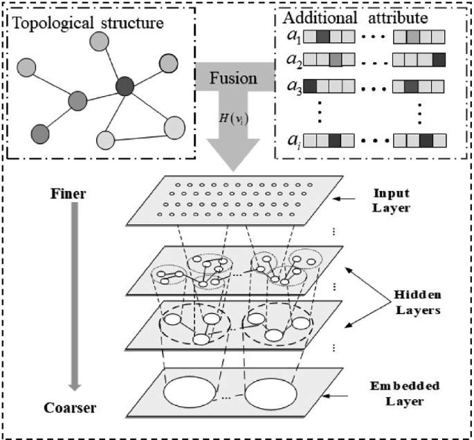
The architecture of the proposed MNRL model.

Firstly, the topology and additional information are fused through the function H, then the variational encoder is used to learn network representation from fine to coarse. The output of the embedded layer are low-dimensional vectors, which combines the attribute information and the network topology.

Multi-granularity Information Fusion. To better characterize multiple granularity complex networks and solve the problem of nodes with potential associations that cannot be processed through the relationship structure alone, we refine the granularity to additional attributes, and designed an information fusion method, which are defined as follows:

$$\begin{aligned} \begin{aligned}&{x_i} = H\left( {{v_i}} \right) \\&H\left( {{v_i}} \right) = {a_i} + \sum \limits _{{v_j} \in N\left( {{v_i}} \right) } {\frac{{d\left( {{v_j}} \right) }}{{d\left( {{v_i}} \right) }}{w_{ij}}{a_j}} \end{aligned} \end{aligned}$$

(1)

Where ${N\left( {{v_i}} \right) }$ is the neighbors of node ${{v}_{i}}$ in the network, ${{a}_{i}}$ is the attributes associated with node ${{v}_{i}}$. ${w_{ij}} > 0$ for weighted networks and ${w_{ij}} = 1$ for unweighted networks. ${d({v_j})}$ is the degree of node ${{v}_{j}}$. ${x_i}$ contains potential information of multiple granularity information, both the neighbor attribute information and the node itself.

Information Complementarity Capture. To capture complementarity of different granularity hierarchies and avoid the effects of various noises, our model in Fig. 1 is a variational auto-encoder, which is a powerful unsupervised deep model for feature learning. It has been widely used for multi-granularity cognitive computing applications. In multi-granularity complex networks, auto-encoders fuse different granularity data to a unified granularity space from fine to coarse. The variational auto-encoder contains three layers, namely, the input layer, the hidden layer, and the output layer, which are defined as follows:

$$\begin{aligned} \begin{aligned}&y_i^1 = \sigma \left( {{w^{\left( 1 \right) }}{x_i} + {b^{\left( 1 \right) }}} \right) \\&y_i^k = \sigma \left( {{w^{\left( k \right) }}y_i^{k - 1} + {b^{\left( k \right) }}} \right) ,k = 2, \ldots ,K - 2\\&{y_\mu } = {w^{\left( {K - 1} \right) }}y_i^k + {b^{\left( {K - 1} \right) }},{y_\sigma } = {w^{\left( {K - 1} \right) }}y_i^k + {b^{\left( {K - 1} \right) }}\\&{y_i^K} = \sigma \left( {{y_\mu } + E*{y_\sigma }} \right) \end{aligned} \end{aligned}$$

(2)

Here, K is the number of layers for the encoder and decoder. $\sigma \left( \cdot \right)$ represents the possible activation functions such as ReLU, sigmod or tanh. ${{w}^{k}}$ and ${{b}^{k}}$ are the transformation matrix and bias vector in the k-th layer, respectively. $y_i^K$ is the unified vector representation that learning from model, which obeys the distribution function E, reducing the influence of noise. $E\sim (0,1)$ is the standard normal distribution in this paper. In order to make the learned representation as similar as possible to the given distribution,it need to minimize the following loss function:

$$\begin{aligned} {L_{KL}} = y_\mu ^2 + y_\sigma ^2 - \log \left( {y_\sigma ^2} \right) - 1 \end{aligned}$$

(3)

To reduce potential information loss of original network, our goal is to minimize the following auto-encoder loss function:

$$\begin{aligned} {L_{RE}} = \mathop \sum \limits _i^n \left\| {{{\hat{x}}_i} - {x_i}} \right\| _2^2 \end{aligned}$$

(4)

where ${{\hat{x}}_{i}}$ is the reconstruction output of decoder and ${x_i}$ incorporates prior knowledge into the model.

Semantic Similarity Preservation. To formulate the homogeneous network structure information, skip-gram model has been widely adopted in recent works and in the field of heterogeneous network research, Skip-grams suitable for different types of nodes processing have also been proposed [32]. In our model, the context of a node is the low-dimensional potential information. Given the node ${{v}_{i}}$ and the associated reconstruction information ${{y}_{i}}$, we randomly walk $c\in C$ by maximizing the loss function:

$$\begin{aligned} {L_{HS}} = \arg \mathrm{{max}}\mathop \sum \limits _{i = 1}^n \mathop \sum \limits _{c \in C} \mathop \sum \limits _{j \le \left| B \right| ,j \ne 0} logp\left( {{v_{i + j}}|{y_i}} \right) \end{aligned}$$

(5)

Where B is the size of the generation window and the conditional probability $p\left( {{v}_{i+j}}|{{y}_{i}} \right)$ is defined as the Softmax function:

$$\begin{aligned} p\left( {{v_{i + j}}|{y_i}} \right) = \frac{{{e^{v_{i + j}^{'T}{y_i}}}}}{{\mathop \sum \nolimits _{k = 1}^n {e^{v_k^{'T}{y_i}}}}} \end{aligned}$$

(6)

In the above formula, $v_{i}^{'}$ is the node context representation of node ${{v}_{i}}$, and ${{y_i}}$ is the result produced by the auto-encoder. Directly optimizing Eq. (6) is computationally expensive, which requires the summation over the entire set of nodes when computing the conditional probability of $p\left( {{v}_{i+j}}|{{y}_{i}} \right)$. We adopt the negative sampling approach proposed in Metapath2vec++ that samples multiple negative samples according to some noisy distributions:

$$\begin{aligned} \log \sigma \left( {v_{i + j}^{'T}{y_i}} \right) + \sum \limits _{t = 1}^S {{E_{v \sim {P_n}\left( v \right) }}\left[ {\log \sigma \left( { - v_n^{'T}{y_i}} \right) } \right] } \end{aligned}$$

(7)

Where $\sigma (\cdot )=1/(1+\exp (\cdot ))$ is the sigmoid function and S is the number of negative samples. We set ${{P}_{n}}\left( v \right) \propto d_{v}^{\frac{3}{4}}$ as suggested in Wode2vec, where ${{d}_{v}}$ is the degree of node ${{v}_{i}}$ [24, 32]. Through the above methods, the node’s attribute information and the heterogeneity of the node’s global structure are processed and the potential semantic similarity kept in a unified granularity space.

MNRL Model Joint Optimization. Multi-granularity complex network representation learning through the fusion of multiple kinds of granularity information, learning the basic granules through an autoencoder, and representing different levels of granularity in a unified low-dimensional vector solves the potential semantic similarity between nodes without direct edges. The model simultaneously optimizes the objective function of each module to make the final result robust and effective. The function is shown below:

$$\begin{aligned} L = \alpha {L_{RE}} + \beta {L_{KL}} + \psi {L_{VAE}} + \gamma \left( { - {L_{HS}}} \right) \end{aligned}$$

(8)

In detail, ${L_{RE}}$ is the auto-encoder loss function of Eq. (4), ${L_{KL}}$ has been stated in formula (3), and ${{L_{HS}}}$ is the loss function of the skip-gram model in Eq. (5). $\alpha ,\beta ,\psi ,\gamma$ are the hyper parameters to balance each module. ${L_{VAE}}$ is the parameter optimization function, the formula is as follows:

$$\begin{aligned} {L_{VAE}} = \frac{1}{2}\sum \limits _{k = 1}^K {(\left\| {{w^k}} \right\| _F^2 + \left\| {{b^k}} \right\| _F^2 + \left\| {{{\hat{w}}^k}} \right\| _F^2 + \left\| {{{\hat{b}}^k}} \right\| _F^2)} \end{aligned}$$

(9)

Where ${{w^k}}$, ${{{\hat{w}}^k}}$ are weight matrices for encoder and decoder respectively in the k-th layer, and ${{b^k}}$, ${{{\hat{b}}^k}}$ are bias matrix. The complete objective function is expressed as follows:

$$\begin{aligned} \begin{aligned} L&= \mathrm{{\alpha }}\mathop \sum \limits _i^n \left\| {{{\hat{x}}_i} - {x_i}} \right\| _2^2\\&+ \beta \left( {y_\mu ^2 + y_\sigma ^2 - log\left( {y_\sigma ^2} \right) - 1} \right) \\&+ \gamma \mathop \sum \limits _{i = 1}^n \mathop \sum \limits _{c \in C} \mathop \sum \limits _{j \le \left| B \right| ,j \ne 0} logp\left( {{v_{i + j}}|{y_i}} \right) \\&+ \frac{\psi }{2}\sum \limits _{k = 1}^K {(\left\| {{w^k}} \right\| _F^2 + \left\| {{b^k}} \right\| _F^2 + \left\| {{{\hat{w}}^k}} \right\| _F^2 + \left\| {{{\hat{b}}^k}} \right\| _F^2)} \end{aligned} \end{aligned}$$

(10)

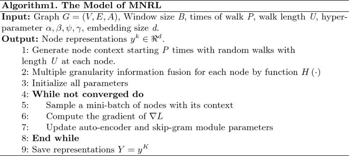
MNRL preserves multiple types of granular information include node attributes, local network structure and global network structure information in a unified framework. The model solves the problems of highly nonlinearity and complementarity of various granularity information, and retained the underlying semantics of topology and additional information at the same time. Finally, we optimize the object function L in Eq. (10) through stochastic gradient descent. To ensure the robustness and validity of the results, we iteratively optimize all components at the same time until the model converges. The learning algorithm is summarized in Algorithm 1.

4 Experiment

4.1 Datasets and Baselines

Datasets: In our experiments, we employ four benchmark datasets: Facebook¹, Cora, Citeseer and PubMed². These datasets contain edge relations and various attribute information, which can verify that the social relations of nodes and individual attributes have strong dependence and indecomposability, and jointly determine the properties of entities in the social environment. The first three datasets are paper citation networks, and these datasets are consist of bibliography publication data. The edge represents that each paper may cite or be cited by other papers. The publications are classified into one of the following six classes: Agents, AI, DB, IR, ML, HCI in Citeseer and one of the three classes (i.e., “Diabetes Mellitus Experimental”, “Diabetes Mellitus Type 1”, “Diabetes Mellitus Type 2”) in Pubmed. The Cora dataset consists of Machine Learning papers which are classified into seven classes. Facebook dataset is a typical social network. Nodes represent users and edges represent friendship relations. We summarize the statistics of these benchmark datasets in Table 1.

Table 1. Statistics of the datasets. ‘-’ indicates unknown labels.

Baselines: To evaluate the performance of our proposed MNRL, we compare it with 9 baseline methods, which can be divided into two groups. The former category of baselines leverage network structure information only and ignore the node attributes contains DeepWalk, Node2Vec, GraRep [33], LINE and SDNE. The other methods try to preserve node attribute and network structure proximity, which are competitive competitors. We consider TADW, GAE, VGAE, DANE as our compared algorithms. For all baselines, we used the implementation released by the original authors. The parameters for baselines are tuned to be optimal. For DeepWalk and Node2Vec, we set the window size as 10, the walk length as 80, the number of walks as 10. For GraRep, the maximum transition step is set to 5. For LINE, we concatenate the first-order and second-order result together as the final embedding result. For the rest baseline methods, their parameters are set following the original papers. At last, the dimension of the node representation is set as 128. For MNRL, the number of layers and dimensions for each dataset are shown in Table 2.

Table 2. Detailed network layer structure information.

4.2 Node Classification

To show the performance of our proposed MNRL, we conduct node classification on the learned node representations. Specifically, we employ SVM as the classifier. To make a comprehensive evaluation, we randomly select 10%, 30%, 50% nodes as the training set and the rest as the testing set respectively. With these randomly chosen training sets, we use five-fold cross validation to train the classifier and then evaluate the classifier on the testing sets. To measure the classification result, we employ Micro-F1 (Mi-F1) and Macro-F1 (Ma-F1) as metrics. The classification results are shown in Table 3, 4, 5 respectively. From these four tables, we can find that our proposed MNRL achieves significant improvement compared with plain network embedding approaches, and beats other attributed network embedding approaches in most situations.

Table 3. Node classification result of Citeseer

Table 4. Node classification result of Cora

Table 5. Node classification result of PubMed

Experimental results show that the representation results of each comparison algorithm perform well in node classification in downstream tasks. In general, a model that considers node attribute information and node structure information performs better than structure alone.

From these three tables, we can find that our proposed MNRL achieves significant improvement compared with single granularity network embedding approaches. For joint representation, our model performs more effectively than most similar types of algorithms, especially in the case of sparse data, because our model input is the fusion information of multiple nodes with extra information. When comparing DANE, our experiments did not improve significantly but it achieved the expected results. DANE uses two auto-encoders to learn and express the network structure and attribute information separately, since the increase of parameters makes the optimal selection in the learning process, the performance will be better with the increase of training data, but the demand for computing resources will also increase and the interpretability of the algorithm is weak. While MNRL uses a variational auto-encoder to learn the structure and attribute information at the same time, the interdependence of information is preserved, which handles heterogeneous information well and reduces the impact of noise.

4.3 Link Prediction

In this subsection, we evaluate the ability of node representations in reconstructing the network structure via link prediction, aiming at predicting if there exists an edge between two nodes, is a typical task in networks analysis. Following other model works do, to evaluate the performance of our model, we randomly holds out 50% existing links as positive instances and sample an equal number of non-existing links. Then, we use the residual network to train the embedding models. Specifically, we rank both positive and negative instances according to the cosine similarity function. To judge the ranking quality, we employ the AUC to evaluate the ranking list and a higher value indicates a better performance. We perform link prediction task on Cora datasets and the results is shown in Fig. 3.

Fig. 3.

Link prediction task on Cora and Facebook datasets

Compared with traditional algorithms that representation learning from a single granular structure information, the algorithms that both on structure and attribute information is more effective. TADW performs well, but the method based on matrix factorization has the disadvantage of high complexity in large networks. GAE and VGAE perform better in this experiment and are suitable for large networks. MNRL refines the input and retains potential semantic information. Link prediction relies on additional information, so it performs better than other algorithms in this experiment.

5 Conclusion

In this paper, we propose a multi-granularity complex network representation learning model (MNRL), which integrates topology structure and additional information, and presents these fused information learning into the same granularity semantic space that through fine-to-coarse to refine the complex network. The effectiveness has been verified by extensive experiments, shows that the relation of nodes and additional attributes are indecomposable and complementarity, which together jointly determine the properties of entities in the network. In practice, it will have a good application prospect in large information network. Although the model saves a lot of calculation cost and well represents complex networks of various granularity, it needs to set different parameters in different application scenarios, which is troublesome and needs to be optimized in the future. The multi-granularity complex network representation learning also needs to consider the dynamic network and adapt to the changes of network nodes, so as to realize the real-time information network analysis.

References

Marsden, P.V., Lin, N. (eds.): Social Structure and Network Analysis, pp. 201–218. Sage, Beverly Hills (1982)
Zhang, D., Yin, J., Zhu, X., Zhang, C.: Network representation learning: a survey. IEEE Trans. Big Data. 6(1), 3–28 (2020)
Fischer, A., Botero, J.F., Beck, M.T., De Meer, H., Hesselbach, X.: Virtual network embedding: a survey. IEEE Commun. Surv. Tutor. 15(4), 1888–1906 (2013)
Liben-Nowell, D., Kleinberg, J.: The link-prediction problem for social networks. J. Am. Soc. Inform. Sci. Technol. 58(7), 1019–1031 (2007)
Wang, F., Li, T., Wang, X., Zhu, S., Ding, C.: Community discovery using nonnegative matrix factorization. Data Min. Knowl. Disc. 22(3), 493–521 (2011)
Bhagat, S., Cormode, G., Muthukrishnan, S.: Node classification in social networks. In: Aggarwal, C. (ed.) Social Network Data Analytics, pp. 115–148. Springer, Boston (2011). https://doi.org/10.1007/978-1-4419-8462-3_5
Resnick, P., Varian, H.R.: Recommender systems. Commun. ACM 40(3), 56–58 (1997)
Perozzi, B., Al-Rfou, R., Skiena, S.: Deepwalk: online learning of social representations. In: Proceedings of the 20th ACM SIGKDD International Conference on Knowledge Discovery and Data Mining, pp. 701–710 (2014)
Grover, A., Leskovec, J.: node2vec: scalable feature learning for networks. In: Proceedings of the 22nd ACM SIGKDD International Conference on Knowledge Discovery and Data Mining, pp. 855–864 (2016)
Tang, J., Qu, M., Wang, M., Zhang, M., Yan, J., Mei, Q.: Line: large-scale information network embedding. In: Proceedings of the 24th International Conference on World Wide Web, pp. 1067–1077 (2015)
LeCun, Y., Bengio, Y., Hinton, G.: Deep learning. Nature 521(7553), 436–444 (2015)
Gao, H., Huang, H.: Deep attributed network embedding. In: IJCAI 2018, pp. 3364–3370 (2018)
Wang, D., Cui, P., Zhu, W.: Structural deep network embedding. In: Proceedings of the 22nd ACM SIGKDD International Conference on Knowledge Discovery and Data Mining, pp. 1225–1234 (2016)
Kipf, T.N., Welling, M.: Semi-supervised classification with graph convolutional networks. arXiv preprint arXiv:1609.02907 (2016)
Wang, G.: DGCC: data-driven granular cognitive computing. Granular Comput. 2(4), 343–355 (2017). https://doi.org/10.1007/s41066-017-0048-3
Bargiela, A., Pedrycz, W.: Granular computing. In: Handbook on Computational Intelligence: Volume 1: Fuzzy Logic, Systems, Artificial Neural Networks, and Learning Systems, pp. 43–66 (2016)
Lin, T.Y., Yao, Y.Y., Zadeh, L.A. (eds.) Data Mining, Rough Sets and Granular Computing, vol. 95. Physica (2013)
Tu, K., Cui, P., Wang, X., Wang, F., Zhu, W.: Structural deep embedding for hyper-networks. In: Thirty-Second AAAI Conference on Artificial Intelligence (2018)
Wold, S., Esbensen, K., Geladi, P.: Principal component analysis. Chemometr. Intell. Lab. Syst. 2(1–3), 37–52 (1987)
Balasubramanian, M., Schwartz, E.L.: The isomap algorithm and topological stability. Science 295(5552), 7 (2002)
Cox, T.F., Cox, M.A.: Multidimensional Scaling. Chapman and Hall/CRC, Boca Raton (2000)
Belkin, M., Niyogi, P.: Laplacian eigenmaps for dimensionality reduction and data representation. Neural Comput. 15(6), 1373–1396 (2003)
Zhang, L., Qian, F., Zhao, S., et al.: Network representation learning based on multi-granularity structure. CAAI Trans. Intell. Syst. 14(6), 1233–1242 (2019). https://doi.org/10.11992/tis.201905045
Goldberg, Y., Levy, O.: word2vec explained: deriving Mikolov et al’.s negative-sampling word-embedding method. arXiv preprint arXiv:1402.3722 (2014)
Chen, H., Perozzi, B., Hu, Y., Skiena, S.: Harp: hierarchical representation learning for networks. In: Thirty-Second AAAI Conference on Artificial Intelligence (2018)
Ng, A.: Sparse autoencoder. In: CS294A Lecture notes, vol. 72, pp. 1–19 (2011)
Yang, C., Liu, Z., Zhao, D., Sun, M., Chang, E.: Network representation learning with rich text information. In: Twenty-Fourth International Joint Conference on Artificial Intelligence (2015)
Sun, X., Guo, J., Ding, X., Liu, T.: A general framework for content-enhanced network representation learning. arXiv preprint arXiv:1610.02906 (2016)
Zhang, Z., et al.: ANRL: attributed network representation learning via deep neural networks. In: IJCAI, vol. 18, pp. 3155–3161 (2018)
Wang, G., Xu, J.: Granular computing with multiple granular layers for brain big data processing. Brain Inform. 1(4), 1–10 (2014). https://doi.org/10.1007/s40708-014-0001-z
Chang, L.Y., Wang, G.Y., Wu, Y.: An approach for attribute reduction and rule generation based on rough set theory. J. Softw. 10(11), 1206–1211 (1999)
Dong, Y., Chawla, N.V., Swami, A.: metapath2vec: scalable representation learning for heterogeneous networks. In: Proceedings of the 23rd ACM SIGKDD International Conference on Knowledge Discovery and Data Mining, pp. 135–144 (2017)
Cao, S., Lu, W., Xu, Q.: GraRep: learning graph representations with global structural information. In: Proceedings of the 24th ACM International on Conference on Information and Knowledge Management, pp. 891–900 (2015)
Meng, Z., Liang, S., Bao, H., Zhang, X.: Co-embedding attributed networks. In: Proceedings of the Twelfth ACM International Conference on Web Search and Data Mining, pp. 393–401 (2019)
Acknowledgments
This work is supported by the National Key Research and Development Program of China under Grant 2017YFC0804002, the National Natural Science Foundation of China (No. 61936001, No. 61772096).
Author information
Authors and Affiliations
Corresponding author
Editor information
Editors and Affiliations
Rights and permissions
Copyright information
© 2020 Springer Nature Switzerland AG
About this paper
Cite this paper
Li, P., Wang, G., Hu, J., Li, Y. (2020). Multi-granularity Complex Network Representation Learning. In: Bello, R., Miao, D., Falcon, R., Nakata, M., Rosete, A., Ciucci, D. (eds) Rough Sets. IJCRS 2020. Lecture Notes in Computer Science(), vol 12179. Springer, Cham. https://doi.org/10.1007/978-3-030-52705-1_18
Download citation
DOI: https://doi.org/10.1007/978-3-030-52705-1_18
Published:
Publisher Name: Springer, Cham
Print ISBN: 978-3-030-52704-4
Online ISBN: 978-3-030-52705-1
eBook Packages: Computer ScienceComputer Science (R0)