ALBATROSS: Publicly AttestabLe BATched Randomness Based On Secret Sharing

Abstract

In this paper we present ALBATROSS, a family of multiparty randomness generation protocols with guaranteed output delivery and public verification that allows to trade off corruption tolerance for a much improved amortized computational complexity. Our basic stand alone protocol is based on publicly verifiable secret sharing (PVSS) and is secure under in the random oracle model under the decisional Diffie-Hellman (DDH) hardness assumption. We also address the important issue of constructing Universally Composable randomness beacons, showing two UC versions of Albatross: one based on simple UC NIZKs and another one based on novel efficient “designated verifier” homomorphic commitments. Interestingly this latter version can be instantiated from a global random oracle under the weaker Computational Diffie-Hellman (CDH) assumption. An execution of ALBATROSS with n parties, out of which up to $t=(1/2-\epsilon )\cdot n$ are corrupt for a constant $\epsilon >0$, generates $\varTheta (n^2)$ uniformly random values, requiring in the worst case an amortized cost per party of $\varTheta (\log n)$ exponentiations per random value. We significantly improve on the SCRAPE protocol (Cascudo and David, ACNS 17), which required $\varTheta (n^2)$ exponentiations per party to generate one uniformly random value. This is mainly achieved via two techniques: first, the use of packed Shamir secret sharing for the PVSS; second, the use of linear t-resilient functions (computed via a Fast Fourier Transform-based algorithm) to improve the randomness extraction.

B. David—Work partially done while visiting IMDEA Software Institute. This work was supported by a grant from Concordium Foundation, DFF grant number 9040-00399B (TrA$^{2}$C) and Protocol Labs grant S$^{2}$LEDGE.

1 Introduction

Randomness is essential for constructing provably secure cryptographic primitives and protocols. While in many cases it is sufficient to assume that each party executing a cryptographic construction has access to a local trusted source of unbiased uniform randomness, many applications (e.g. electronic voting  [1] and anonymous messaging  [35, 36]) require a randomness beacon  [30] that can periodically provide fresh random values to all parties. Constructing such a randomness beacon without relying on a trusted third party requires a multiparty protocol that can be executed in such a way that all parties are convinced that an unbiased random value is obtained after the execution terminates, even if a fraction of these parties are corrupted. Moreover, in certain scenarios (e.g. in electronic voting  [1]) it might be necessary to employ a publicly verifiable randomness beacon, which allows for third parties who did not participate in the beacon’s execution to verify that indeed a given random value was successfully obtained after a certain execution. To raise the challenge of constructing such randomness beacons even more, there are classes of protocols that require a publicly verifiable randomness beacon with guaranteed output delivery, meaning that the protocol is guaranteed to terminate and output an unbiased random value no matter what actively corrupted parties do. A prominent class of protocols requiring publicly verifiable randomness beacons with guaranteed output delivery is that of Proof-of-Stake based blockchain consensus protocols  [18, 23], which are the main energy-efficient alternative to wasteful Proof-of-Work based blockchain consensus protocols  [21, 25].

Related Works: A number of randomness beacons aiming at being amenable to blockchain consensus applications have been proposed based on techniques such as Verifiable Delay Functions (VDF)  [6], randomness extraction from data in the blockchain  [2], Publicly Verifiable Secret Sharing  [12, 23, 33] or Verifiable Random Functions  [15, 18]. However, most of these schemes do not guarantee either the generation of perfectly uniformly random values  [2, 15, 18] or that a value will be generated regardless of adversarial behavior  [33]. Those methods that do have those two guarantees suffer from high computational and communication complexity  [23] or even higher computational complexity in order to improve communication complexity  [6]. Another issue with VDF based approaches is that their security relies on very precise estimates of the average concrete complexity of certain computational tasks (i.e. how much time it takes an adversary to compute a VDF), which are hard to obtain for real world systems. While SCRAPE  [12] does improve on  [23], it can still be further improved, as is the goal of this work. Moreover, none of the protocols that guarantee generation of truly unbiased uniformly random values have any composability guarantees. This is a very important issue, since these protocols are not used in isolation but as building blocks of more complex systems and thus need composability.

Our Contributions: We present ALBATROSS, a family of multiparty randomness generation protocol with guaranteed output delivery and public verification, where parties generate $\varTheta (n^2)$ independent and uniformly random elements in a group and where the computational complexity for each party in the worst case is of $\varTheta (\log n)$ group exponentiations (the most computationally expensive operation in the protocol) per random element generated, as long as the number of corrupted parties is $t=n/2-\varTheta (n)$. Our contributions are summarized below:

• The first randomness beacon with $\varTheta (\log n)$ group exponentiations per party.

• The first Universally Composable randomness beacon producing unbiased uniformly random values.

• The first randomness beacon based on the Computational Diffie-Hellman (CDH) assumption via novel “designated verifier” homomorphic commitments, which might be of independent interest.

Our basic stand alone protocol builds on SCRAPE  [12], a protocol based on publicly verifiable secret sharing (PVSS). We depart from the variant of SCRAPE based on the Decisional Diffie-Hellman (DDH) assumption, which required $\varTheta (n^2)$ group exponentiations per party to generate just one uniformly random element in the group, but tolerated any dishonest minority. Therefore, what we obtain is a trade-off of corruption tolerance in exchange for a much more efficient randomness generation, under the same assumptions (DDH hardness, RO model). We gain efficiency for ALBATROSS in the suboptimal corruption scenario by introducing two main techniques on top of SCRAPE, that in fact can be applied independently from each other: the first one is the use of “packed” (or “ramp”) Shamir secret sharing in the PVSS, and the second is the use of privacy amplification through t-resilient functions that allows to extract more uniform randomness from a vector of group elements from which the adversary may control some of the coordinates. Applying these techniques requires us to overcome significant obstacles (see below) but using them together allows ALBATROSS to achieve the complexity of $\varTheta (\log n)$ exponentiations per party and random group element. Moreover, this complexity is worst case: the $\log n$ factor only appears if a large number of parties refuse to open the secrets they have committed to, thereby forcing the PVSS reconstruction on many secrets, and a less efficient output phase. Otherwise (if e.g. all parties act honestly) the amortized complexity is of O(1) exponentiation per party and element generated.

Our Techniques: In order to create a uniformly random element in a group in a multiparty setting, a natural idea is to have every party select a random element of that group and then have the output be the group operation applied to all those elements. However, the last party in acting can see the choices of the other parties and change her mind about her input, so a natural solution is to have every party commit to their random choice first. Yet, the adversary can still wait until everyone else has opened their commitments and decide on whether they want to open or not based on the observed result, which clearly biases the output. In order to solve this, we can have parties commit to the secrets by using a publicly verifiable secret sharing scheme to secret-share them among the other parties as proposed in  [12, 23]. The idea is that public verifiability guarantees that the secret will be able to be opened even if the dealer refuses to reveal the secrets. The final randomness is constructed from all these opened secrets.

In the case of SCRAPE the PVSS consists in creating Shamir shares $\sigma _i$ for a secret s in a finite field $\mathbb {Z}_q$, and publishing the encryption of $\sigma _i$ under the public key $pk_i$ of party i. More concretely, the encryption is $pk_i^{\sigma _i}$, and $pk_i=h^{sk_i}$ for h a generator of a DDH-hard group $\mathbb {G}_q$ of cardinality q; what party i can decrypt is not really the Shamir share $\sigma _i$, but rather $h^{\sigma _i}$. However these values are enough to reconstruct $h^s$ which acts as a uniformly random choice in the group by the party who chose s. The final randomness is $\prod h^{s^a}$. Public verifiability of the secret sharing is achieved in SCRAPE by having the dealer commit to the shares independently via some other generator g of the group (i.e. they publish $g^{\sigma _i}$), proving that these commitments contain the same Shamir shares via discrete logarithm equality proofs, or DLEQs, and then having verifiers use a procedure to check that the shares are indeed evaluations of a low-degree polynomial. In this paper we will use a different proof, but we remark that the latter technique, which we call $Local_{LDEI}$ test, will be of use in another part of our protocol (namely it is used to verify that $h^s$ is correctly reconstructed).

In ALBATROSS we assume that the adversary corrupts at most t parties where $n-2t=\ell =\varTheta (n)$. The output of the protocol will be $\ell ^2$ elements of $\mathbb {G}_q$.

Larger Randomness via Packed Shamir Secret Sharing. In this suboptimal corruption scenario, we can use packed Shamir secret sharing, which allows to secret-share a vector of $\ell$ elements from a field (rather than a single element). The key point is that every share is still one element of the field and therefore the sharing has the same computational cost ($\varTheta (n)$ exponentiations) as using regular Shamir secret sharing. However, there is still a problem that we need to address: the complexity of the reconstruction of the secret vector from the shares increases by the same factor as the secret size (from $\varTheta (n)$ to $\varTheta (n^2)$ exponentiations). To mitigate this we use the following strategy: each secret vector will be reconstructed only by a random subset of c parties (independently of each other). Verifying that a reconstruction is correct only requires $\varTheta (n)$ exponentiations, by using the aforementioned $Local_{LDEI}$. The point is that if we assign $c=\log n$, then with large probability there will be only at most a small constant number of secret tuples that were not correctly reconstructed by any of the c(n) parties and therefore it does not add too much complexity for the parties to compute those. The final complexity of this phase is then $O(n^2\log n)$ exponentiations for each party, in the worst case.

Larger Randomness via Resilient Functions. To simplify, let us first assume that packed secret sharing has not been used. In that case, right before the output phase from SCRAPE, parties will know a value $h^{s_a}$ for each of the parties $P_a$ in the set $\mathcal {C}$ of parties that successfully PVSS’ed their secrets (to simplify, let us say $\mathcal {C}=\{P_1,P_2,\dots ,P_{|\mathcal {C}|}\}$), where h is a generator of a group of order q. In the original version of SCRAPE, parties then compute the final randomness as $\prod _{a=1}^{|\mathcal {C}|} h^{s_a}$, which is the same as $h^{\sum _{a=1}^{|\mathcal {C}|} s_a}$.

Instead, in ALBATROSS, we use a randomness extraction technique based on a linear t-resilient function, given by a matrix M, in such a way that the parties instead output a vector of random elements $(h^{r_1}$, ..., $h^{r_m})$ where $(r_1,...,r_m)=M (s_{1},\dots ,s_{|\mathcal {C}|})$. The resilient function has the property that the output vector is uniformly distributed as long as $|\mathcal {C}|-t$ inputs are uniformly distributed, even if the other t are completely controlled by the adversary. If in addition packed secret sharing has been used, one can simply use the same strategy for each of the $\ell$ coordinates of the secret vectors created by the parties. In this way we can create $\ell ^2$ independently distributed uniformly random elements of the group.

An obstacle to this randomness extraction strategy is that, in the presence of corrupted parties some of the inputs $s_i$ may not be known if the dealers of these values have refused to open them, since PVSS reconstruction only allows to retrieve the values $h^{s_i}$. Then the computation of the resilient function needs to be done in the exponent which in principle appears to require either $O(n^3)$ exponentiations, or a distributed computation like in the PVSS reconstruction.

Fortunately, in this case the following idea allows to perform this computation much more efficiently: we choose M to be certain type of Vandermonde matrix so that applying M is evaluating a polynomial (with coefficients given by the $s_i$) on several n-th roots of unity. Then we adapt the Cooley-Tukey fast Fourier transform algorithm to work in the exponent of the group and compute the output with $n^2\log n$ exponentiations, which in practice is almost as fast as the best-case scenario where the $s_i$ are known. This gives the claim amortized complexity of $O(\log n)$ exponentiations per party and random element computed.

Additional Techniques to Decrease Complexity. We further reduce the complexity of the PVSS used in ALBATROSS, with an idea which can also be used in SCRAPE [12]. It concerns public verification that a published sharing is correct, i.e. that it is of the form $pk_i^{p(i)}$ for some polynomial of bounded degree, say at most k. Instead of the additional commitment to the shares used in [12], we use standard $\varSigma$-protocol ideas that allow to prove this type of statement, which turns out to improve the constants in the computational complexity. We call this type of proof a low degree exponent interpolation (LDEI) proof.

Universal Composability. We extend our basic stand alone protocol to obtain two versions that are secure in the Universal Composability (UC) framework  [10], which is arguably one of the strongest security guarantees one can ask from a protocol. In particular, proving a protocol UC secure ensures that it can be used as a building block for more complex systems while retaining its security guarantees, which is essential for randomness beacons. We obtain the first UC-secure version of ALBATROSS by employing UC non-interactive zero knowledge proofs (NIZKs) for discrete logarithm relations, which can be realized at a reasonable overhead. The second version explores a new primitive that we introduce and construct called “designated verifier” homomorphic commitments, which allows a sender to open a commitment towards one specific receiver in such a way that this receiver can later prove to a third party that the opening revealed a certain message. Instead of using DDH based encryption schemes as before, we now have the parties commit to their shares using our new commitment scheme and rely on its homomorphic properties to perform the LDEI proofs that ensure share validity. Interestingly, this approach yields a protocol secure under the weaker CDH assumption in the random oracle model.

2 Preliminaries

[n] denotes the set $\{1,2,\dots ,n\}$ and [m, n] denotes the set $\{m,m+1,\dots ,n\}$. We denote vectors with black font lowercase letters, i.e. $\mathbf {v}$. Given a vector $\mathbf {v}=(v_1,\dots ,v_n)$ and a subset $I\subseteq [n]$, we denote by $\mathbf {v}_I$ the vector of length |I| with coordinates $v_i, i\in I$ in the same order they are in $\mathbf {v}$. Throughout the paper, q will be a prime number and $\mathbb {Z}_q=\mathbb {Z}/q\mathbb {Z}$ is a finite field of q elements. For a field $\mathbb {F}$, $\mathbb {F}^{m\times n}$ is the set of $m\times n$ matrices with coefficients in $\mathbb {F}$. Moreover, we denote by $\mathbb {F}[X]_{\le m}$ the vector space of polynomials in $\mathbb {F}[X]$ with degree at most m. For a set $\mathcal {X}$, let $x \, {\mathop {\leftarrow }\limits ^{{\scriptscriptstyle \$}}}\, \mathcal {X}$ denote x chosen uniformly at random from $\mathcal {X}$; and for a distribution $\mathcal {Y}$, let $y \, {\mathop {\leftarrow }\limits ^{{\scriptscriptstyle \$}}}\, \mathcal {Y}$ denote y sampled according to the distribution $\mathcal {Y}$.

Polynomial Interpolation and Lagrange Basis. We recall a few well known facts regarding polynomial interpolation in fields.

Definition 1 (Lagrange basis)

Let $\mathbb {F}$ be a field, and $S=\{a_1,\dots ,a_r\}\subseteq \mathbb {F}$. A basis of $\mathbb {F}[X]_{\le r-1}$, called the Lagrange basis for S, is given by $\{L_{a_i,S}(X): i\in [r]\}$ defined by

$$L_{a_i,S}(X)=\prod _{a_j\in S\setminus \{a_i\}} \frac{X-a_j}{a_i-a_j}.$$

Lemma 1

Let $\mathbb {F}$ be a field, and $S=\{a_1,\dots ,a_r\}\subseteq \mathbb {F}$. Then the map $\mathbb {F}[X]_{\le r-1}\rightarrow \mathbb {F}^{r}$ given by $f(X)\mapsto (f(a_1),\dots ,f(a_r))$ is a bijection, and the preimage of $(b_1,\dots ,b_r)\in \mathbb {F}^r$ is given by $f(X)=\sum _{i=1}^r b_i\cdot L_{a_i,S}(X)$.

Packed Shamir Secret Sharing. From now on we work on the finite field $\mathbb {Z}_q$. Shamir secret sharing scheme  [32] allows to share a secret $s\in \mathbb {Z}_q$ among a set of n parties (where $n<q$) so that for some specified $1\le t<n$, the secret can be reconstructed from any set of $t+1$ shares via Lagrange interpolation ($t+1$-reconstruction), while any t or less shares convey no information about it (t-privacy). In Shamir scheme each share is also in $\mathbb {Z}_q$ and therefore of the same size of the secret.

Packed Shamir secret sharing scheme  [5, 20] is a generalization that allows for sharing a vector in $\mathbb {Z}_q^\ell$ while each share is still one element of $\mathbb {Z}_q$. Standard Shamir is the case $\ell =1$. Packing comes at the inevitable cost of sacrificing the threshold nature of Shamir’s scheme, which is replaced by an (optimal) quasithreshold (often called “ramp”) behavior, namely there is t-privacy and $t+\ell$ reconstruction. The description of the sharing and reconstruction (from $t+\ell$ shares) algorithms can be found in Fig. 1.

Fig. 1.

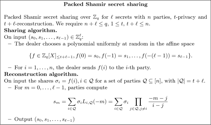
Packed Shamir secret sharing (sharing algorithm)

Remark 1

The points $0,-1,\dots ,-(\ell -1)$ (for the secret) and $1,\dots ,n$ (for the shares) can be replaced by any set of $n+\ell$ pairwise distinct points. In this case the reconstruction coefficients should be changed accordingly. Choosing other evaluation points may be beneficial due to efficient algorithms for both computing the shares and the Lagrange coefficients [34]. In this work we will not focus on optimizing this aspect and use the aforementioned points for notational simplicity.

Linear Codes. The Hamming weight of a vector $\mathbf {c}\in \mathbb {Z}_q^n$ is the number of nonzero coordinates of $\mathbf {c}$. An $[n, k, d]_q$-linear error correcting code C is a vector subspace of $\mathbb {Z}_q^n$ of dimension k and minimum distance d, i.e., the smallest Hamming weight of a nonzero codeword in C is exactly d. A generator matrix is a matrix $M\in \mathbb {Z}_q^{k\times n}$ such that $C=\{\mathbf {m}\cdot M: \mathbf {m}\in \mathbb {Z}_q^k\}$.

Given n pairwise distinct points $x_1,\dots , x_n$ in $\mathbb {Z}_q^n$, a Reed Solomon of length n and dimension k is defined as $=\{(f(x_1),\dots ,f(x_n)): f\in \mathbb {Z}_q[X], \deg f<k\}.$ It is well known that this is an $[n,k,n-k+1]_q$-linear code, and therefore achieves the largest possible minimum distance for a code of that length and dimension. These codes are called MDS (maximum distance separable).

The dual code of a code C, denoted $C^{\bot }$, is the vector space consisting of all vectors $\mathbf {c}^{\bot }\in \mathbb {Z}_q^n$ such that $\langle \mathbf {c}, \mathbf {c}^{\bot }\rangle =0$ for all $\mathbf {c}\in C$ where $\langle \cdot , \cdot \rangle$ denotes the standard inner product. For the Reed-Solomon code above, its dual is the following so-called generalized Reed-Solomon code

$$C^{\bot }=\{(u_1\cdot f_*(x_1),\dots ,u_n\cdot f_*(x_n)):g\in \mathbb {Z}_q[X], \deg f_*<n-k\}$$

where $u_1,...,u_n$ are fixed elements of $\mathbb {Z}_q^n$, namely $u_i=\prod _{j=1, j\ne i}^n (x_i-x_j)^{-1}$.

Linear Perfect Resilient Functions. Our optimizations make use of randomness extractors which are linear over $\mathbb {Z}_q$ and hence given by a matrix $M\in \mathbb {Z}_q^{u\times r}$ satisfying the following property: the knowledge of any t coordinates of the input gives no information about the output (as long as the other $r-t$ coordinates are chosen uniformly at random). This notion is known as linear perfect t-resilient function [16].

Definition 2

A $\mathbb {Z}_q$-linear (perfect) t-resilient function (t-RF for short) is a linear function $\mathbb {Z}_q^r\rightarrow \mathbb {Z}_q^u$ given by $\mathbf {x}\mapsto M\cdot \mathbf {x}$ such that for any $I\subseteq [r]$ of size t, and any $\mathbf {a}_I=(a_j)_{j\in I}\in \mathbb {Z}_q^{t}$, the distribution of $M\cdot \mathbf {x}$ conditioned to $\mathbf {x}_I=\mathbf {a}_I$ and to $\mathbf {x}_{[r]\setminus I}$ being uniformly random in $\mathbb {Z}_q^{r-t}$, is uniform in $\mathbb {Z}_q^u$.

Note that such a function can only exist if $u\le r-t$. We have the following characterization in terms of linear codes.

Theorem 1

[16]. An $u\times r$ matrix M induces a linear t-RF if and only if M is a generator matrix for an $[r,u,t+1]_q$-linear code.

Remark 2

Remember that with our notation for linear codes, the generator matrix acts on the right for encoding a message, i.e. $\mathbf {m}\mapsto \mathbf {m}\cdot M$. In other words the encoding function for the linear code and the corresponding resilient function given by the generator matrix as in Theorem 1 are “transpose from each other”.

A t-RF for the optimal case $u=r-t$ is given by any generator matrix of an $[r,r-t,t+1]_q$ MDS code, for example a matrix M with $M_{ij}=a_j^{i-1}$ for $i\in [r-t]$, $j\in [r]$, where all $a_j$’s are distinct, which generates a Reed-Solomon code. It will be advantageous for us to fix an element $\omega \in \mathbb {Z}_q^*$ of order at least $r-t$ and set $a_j=\omega ^{j-1}$, that is we will use the matrix $M=M(\omega ,r-t,r)$ where

$$M_{ij}=\omega ^{(i-1)(j-1)}, i\in [r-t], j\in [r]$$

Then $M\cdot \mathbf {x}=(f(1),f(\omega ),\cdots ,f(\omega ^{r-t-1}))$ where $f(X):=x_0+x_1X+x_2X^2+\dots +x_{r-1}X^{r-1}$, and we can use the Fast Fourier transform to compute $M\cdot \mathbf {x}$ very efficiently, as we explain later.

3 Basic Algorithms and Protocols

In this section we introduce some algorithms and subprotocols which we will need in several parts of our protocols, and which are relatively straight-forward modifications of known techniques.

3.1 Proof of Discrete Logarithm Equality

We will need a zero-knowledge proof that given $g_1,...,g_m$ and $x_1,...,x_m$ the discrete logarithms of every $x_i$ with base $g_i$ are equal. That is $x_i = g_i^\alpha$ for all $i\in [m]$ for some common $\alpha \in \mathbb {Z}_q$. Looking ahead, these proofs will be used by parties in the PVSS to ensure they have decrypted shares correctly. A sigma-protocol performing DLEQ proofs for $m=2$ was given in [14]. We can easily adapt that protocol to general m as follows:

• 1. The prover samples $w \leftarrow \mathbb {Z}_q$ and, for all $i\in [m]$, computes $a_i = g_i^w$ and sends $a_i$ to the verifier.

• 2. The verifier sends a challenge $e \leftarrow \mathbb {Z}_q$ to the prover.

• 3. The prover sends a response $z=w-\alpha e$ to the verifier.

• 4. The verifier accepts if $a_i=g_i^z x_i^e$ for all $i\in [m]$.

We transform this proof into a non-interactive zero-knowledge proof of knowledge of $\alpha$ in the random oracle model via the Fiat-Shamir heuristic [19, 29]:

• The prover computes $e=H(g_1,\ldots ,g_m, x_{1},\ldots ,x_{m},a_{1},\ldots ,a_{m}),$ for $H(\cdot )$ a random oracle (that will be instantiated by a cryptographic hash function) and z as above. The proof is $(a_1,\dots ,a_m,e,z)$.

• The verifier checks that $e=H(g_1,\ldots ,g_m, x_{1},\ldots ,x_{m},a_{1},\ldots ,a_{m})$ and that $a_i=g_i^z x_i^e$ for all i.

This proof requires m exponentiations for the prover and 2m for the verifier.

3.2 Proofs and Checks of Low-Degree Exponent Interpolation

We consider the following statement: given generators $g_1,g_2,\dots ,g_m$ of a cyclic group $\mathbb {G}_q$ of prime order q, pairwise distinct elements $\alpha _1,\alpha _2,\dots ,\alpha _m$ in $\mathbb {Z}_q$ and an integer $1\le k<m$, known by prover and verifier, the claim is that a tuple $(x_1,x_2,\dots , x_m)\in \mathbb {G}_q^{m}$ is of the form $(g_1^{p(\alpha _1)},g_2^{p(\alpha _2)},\dots ,g_m^{p(\alpha _m)})$ for a polynomial p(X) in $\mathbb {Z}_q[X]_{\le k}$. We will encounter this statement in two different versions:

• In the first situation, we need a zero-knowledge proof of knowledge of p(X) by the prover. This type of proof will be used for a dealer in the publicly verifiable secret sharing scheme to prove correctness of sharing. We call this proof $LDEI((g_i)_{i\in [m]},(\alpha _i)_{i\in [m]}, k, (x_i)_{i\in [m]})$.

• In the second situation, we have no prover, but on the other hand we have $g_1=g_2=\dots =g_m$. In that case we will use a locally computable check from [12]: indeed, verifiers can check by themselves that the statement is correct with high probability. This type of check will be used to verify correctness of reconstruction of a (packed) secret efficiently. We call such check $Local_{LDEI}((\alpha _i)_{i\in [m]}, k, (x_i)_{i\in [m]}))$.¹

In [12], the first type of proof was constructed by using a DLEQ proof of knowledge of common exponent to reduce that statement to one of the second type and then using the local check we just mentioned. However, this is unnecessarily expensive both in terms of communication and computation. Indeed, a simpler $\varSigma$-protocol for that problem is given in Fig. 2.

Fig. 2.

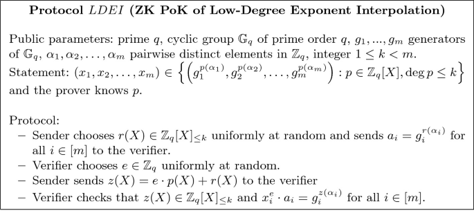
Protocol $LDEI$ zero-knowledge proof of knowledge of low-degree exponent interpolation.

Proposition 1

Protocol $LDEI$ in Fig. 2 is an honest-verifier zero-knowledge proof of knowledge for the given statement.

Proof

The proof of this proposition follows standard arguments in $\varSigma$-protocol theory and is given in the full version of this paper  [13].

Applying Fiat-Shamir heuristic we transform this into a non-interactive proof:

• The sender chooses $r\in \mathbb {Z}_q[X]_{\le k}$ uniformly at random and computes $a_i=g_i^{r(\alpha _i)}$ for all $i=1,\dots ,m$, $e=H(x_1,x_2,\dots ,x_m,a_1,a_2,\dots ,a_m)$ and $z=e\cdot p+r$. The proof is then $(a_1,a_2,\dots ,a_m,e,z)$.

• The verifier checks that $z\in \mathbb {Z}_q[X]_{\le k}$, that $x_i^e\cdot a_i=g_i^{z(\alpha _i)}$ holds for all $i=1,\dots ,m$ and that $e=H(x_1,x_2,\dots ,x_m,a_1,a_2,\dots ,a_m)$.

Now we consider the second type of situation mentioned above. The local check is given in Fig. 3.

Fig. 3.

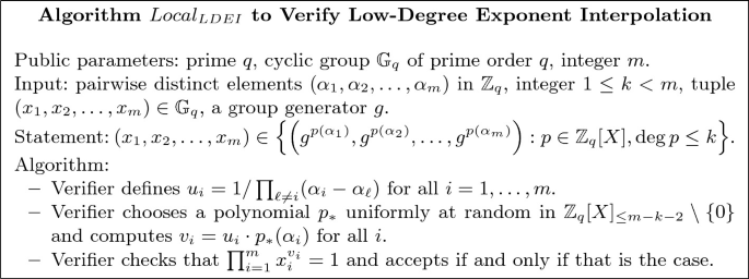
Algorithm $Local_{LDEI}$ to verify low-degree exponent interpolation

Proposition 2

The local test $Local_{LDEI}$ in Fig. 3 always accepts if the statement is true and rejects with probability at least $1-1/q$ if the statement is false.

Correctness is based on the fact that the vector $(u_1 p_*({\alpha _1}),\dots ,u_n p_*(\alpha _m))$ is in the dual code $C^{\bot }$ of the Reed Solomon code C given by the vectors $(p({\alpha _1}),\dots ,p(\alpha _m))$ with deg $p\le k$, hence if the exponents of the $x_i$’s (in base g) indeed form a codeword in C, the verifier is computing the inner product of two orthogonal vectors in the exponent. Soundness follows from the fact that, if the vector is not a codeword in C, then a uniformly random element in $C^{\bot }$ will only be orthogonal to that vector of exponents with probability less than 1/q. See [12, Lemma 1] for more information about this claim.

3.3 Applying Resilient Functions “in the Exponent”

In our protocol we will need to apply resilient functions in the following way. Let $h_1,\dots ,h_r$ be public elements of $\mathbb {G}_q$, chosen by different parties, so that $h_i=h^{x_i}$ (for some certain public generator h of the group) and $x_i$ is only known to the party that has chosen it. Our goal is to extract $(\widehat{h}_1,\dots ,\widehat{h}_u)\in \mathbb {G}_q^u$ which is uniformly random in the view of an adversary who has control over up to t of the initial elements $x_i$. In order to do that, we take a t-resilient function from $\mathbb {Z}_q^r$ to $\mathbb {Z}_q^u$ given by a matrix M and apply it to the exponents, i.e., we define $\widehat{h}_i=h^{y_i}$ where $\mathbf {x}\mapsto \mathbf {y}=M\cdot \mathbf {x}$; this satisfies the desired properties. Because the resilient function is linear, the values $\widehat{h}_i$ can be computed from the $h_i$ by group operations, without needing the exponents $x_i$. We define the following notation.

Definition 3

As above, let $\mathbb {G}_q$ be a group of order q in multiplicative notation. Given a matrix $M=(M_{ij})$ in $\mathbb {Z}_q^{u\times r}$ and a vector $\mathbf {h}=(h_1,h_2,\dots ,h_r)\in \mathbb {G}_q^{r}$, we define $\widehat{\mathbf {h}}=M\diamond \mathbf {h}\in \mathbb {G}_q^{u}$, as $\widehat{\mathbf {h}}=(\widehat{h}_1,\widehat{h}_2,\dots ,\widehat{h}_r)$, where $\widehat{h}_{i}=\prod _{k=1}^{u} h_{k}^{M_{ik}}.$

Remark 3

Given a generator h of $\mathbb {G}_q$, if we write $\mathbf {h}=(h^{x_1},h^{x_2},\dots ,h^{x_r})$, $\mathbf {x}=(x_1,x_2,\dots ,x_r)$, then $M\diamond \mathbf {h}=(h^{y_1},h^{y_2},\dots ,h^{y_r})$ where $(y_1,y_2,\dots ,y_r)=M\cdot \mathbf {x}$.

Now let $M=M(\omega ,r-t,r)$ as in Sect. 2. In order to minimize the number of exponentiations that we need to compute $M\diamond \mathbf {h}$ recall first that $M\cdot \mathbf {x}=(f(1),f(\omega ),\dots ,f(\omega ^{r-t-1}))$, where f is the polynomial with coefficients $f_i=x_{i+1}$, for $i\in [0,r-1]$. Assuming there exists $n>r-t-1$ a power of 2 that divides $q-1$, we can choose $\omega$ to be a n-th root of unity for n and use the well known Cooley-Tukey recursive algorithm  [17] for computing the Fast Fourier Transform. The algorithm in fact evaluates a polynomial of degree up to $n-1$ on all powers of $\omega$ up to $\omega ^{n-1}$ with $O(n \log n)$ multiplications. We can just set $f_j=0$ for $j\ge r$, and ignore the evaluations in $\omega ^i$, for $i\ge r-t$. In our situation the $x_i$’s are not known; we use the fact that in the Cooley-Tukey algorithm all operations on the $x_i$ are linear, so we can operate on the values $h_i=h^{x_i}$ instead. The resulting algorithm is then given in Fig. 4 (since we denoted $f_i=x_{i+1}$, then $h_i=h^{f_{i-1}}$).

Fig. 4.

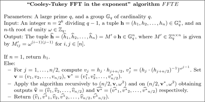
Algorithm $FFTE$ (Cooley-Tukey FFT in the exponent)

At every recursion level of the algorithm, it needs to compute in total n exponentiations, and therefore the total number of exponentiations in $\mathbb {G}_q$ is $n\log _2 n$. In fact, half of these are inversions, which are typically faster.

4 ALBATROSS Protocols

We will now present our main protocols for multiparty randomness generation. We assume n participants, at most $t<(n-1)/2$ of which can be corrupted by some active static adversary. We define then $\ell =n-2t>0$. Note that $n-t=t+\ell$, so we use these two quantities interchangeably. For asymptotics, we consider that both t and $\ell$ are $\varTheta (n)$, in particular $t=\tau \cdot n$ for some $0<\tau <1/2$. The n participants have access to a public ledger, where they can publish information that can be seen by the other parties and external verifiers.

Our protocols take place in a group $\mathbb {G}_q$ of prime cardinality q, where we assume that the Decisional Diffie-Hellman problem is hard. Furthermore, in order to use the FFTE algorithm we require that $\mathbb {G}_q$ has large 2-adicity, i.e., that $q-1$ is divisible by a large power of two $2^u$. Concretely we need $2^u>n-t$. DDH-hard elliptic curve groups with large 2-adicity are known, for example both the Tweedledee and Tweedledum curves from [8] satisfy this property for $u=33$, which is more than enough for any practical application.

4.1 A PVSS Based on Packed Shamir Secret Sharing

As a first step, we show a generalization of a PVSS from [12], where we use packed Shamir secret sharing in order to share several secrets at essentially the same cost for the sharing and public verification phases. In addition, correctness of the shares is instead verified using the $LDEI$ proof. This is different than in [12] where the dealer needed to commit to the shares using a different generator of the group, and correctness of the sharing was proved using a combination of DLEQ proofs and the $Local_{LDEI}$ check, which is less efficient. In Fig. 5, we present the share distribution and verification of the correctness of the shares of the new PVSS. We discuss the reconstruction of the secret later.

Fig. 5.

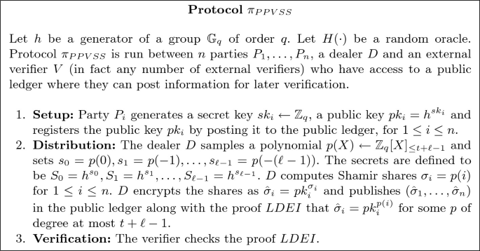
Protocol $\pi _{PPVSS}$

Under the DDH assumption, $\pi _{PPVSS}$ satisfies the property of IND1-secrecy as defined in [12] (adapted from [22, 31]), which requires that given t shares and a vector $\mathbf {x}'=(s'_0,s'_1,\dots ,s'_{\ell -1})$, the adversary cannot tell whether $\mathbf {x}'$ is the actual vector of secrets.

Definition 4

Indistinguishability of secrets (IND1-secrecy). We say that the PVSS is IND1-secret if for any polynomial time adversary $\mathcal {A}_{\text {Priv}}$ corrupting at most $t-1$ parties, $\mathcal {A}_{\text {Priv}}$ has negligible advantage in the following game played against a challenger.

• 1. The challenger runs the Setup phase of the PVSS as the dealer and sends all public information to $\mathcal {A}_{\text {Priv}}$. Moreover, it creates secret and public keys for all honest parties, and sends the corresponding public keys to $\mathcal {A}_{\text {Priv}}$.

• 2. $\mathcal {A}_{\text {Priv}}$ creates secret keys for the corrupted parties and sends the corresponding public keys to the challenger.

• 3. The challenger chooses values $\mathbf {x}_0$ and $\mathbf {x}_1$ at random in the space of secrets. Furthermore it chooses $b\leftarrow \{0,1\}$ uniformly at random. It runs the Distribution phase of the protocol with $x_0$ as secret. It sends $\mathcal {A}_{\text {Priv}}$ all public information generated in that phase, together with $\mathbf {x}_b$.

• 4. $\mathcal {A}_{\text {Priv}}$ outputs a guess $b'\in \{0,1\}$.

The advantage of $\mathcal {A}_{\text {Priv}}$ is defined as $|\Pr [b=b']-1/2|$.

Proposition 3

Protocol $\pi _{PPVSS}$ is IND1-secret under the DDH assumption.

We prove this proposition in the full version of the paper  [13], but we note that the proof follows from similar techniques as in the security analysis of the PVSS in SCRAPE  [12] and shows IND1-secrecy based on the $\ell$-DDH hardness assumption, which claims that given $(g,g^\alpha ,g^{\beta _0},g^{\beta _1},\cdots ,g^{\beta _{\ell -1}}, g^{\gamma _0},g^{\gamma _1},\cdots ,g^{\gamma _{\ell -1}})$ where the $\gamma _i$ either have all been sampled at random from $\mathbb {Z}_q$ or are equal to $\alpha \cdot \beta _i$, it is hard to distinguish both situations. However, when $\ell$ is polynomial in the security parameter (as is the case here) $\ell$-DDH is equivalent to DDH, see  [26].

We now discuss how to reconstruct secrets in $\pi _{PPVSS}$. Rather than giving one protocol, in Fig. 6 we present a number of subprotocols that can be combined in order to reconstruct a secret. The reason is to have some flexibility about which parties will execute the reconstruction algorithm and which ones will verify the reconstruction in the final randomness generation protocol.

In the share decryption protocol party $P_i$, using secret key $sk_i$, decrypts the share $\hat{\sigma }_i$ and publishes the obtained value $h^{\sigma _i}$. Moreover $P_i$ posts a DLEQ proof to guarantee correctness of the share decryption; if several secret tuples need to be reconstructed, this will be done by a batch DLEQ proof.

Once $n-t$ values $h^{\sigma _i}$ have been correctly decrypted (by a set of parties $\mathcal {Q}$), any party can compute the $\ell$ secret values $S_j=h^{s_j}$ using the reconstruction algorithm $Rec_{\mathcal {Q}}$, which boils down to applying Lagrange interpolation in the exponent. Note that since Lagrange interpolation is a linear operation, the exponents $\sigma _i$ do not need to be known, one can operate on the values $h^{\sigma _i}$ instead.

However, the computational complexity of this algorithm is high ($O(n^2)$ exponentiations) so we introduce the reconstruction verification algorithm $RecVer_{\mathcal {Q}}$ which allows any party to check whether a claimed reconstruction is correct at a reduced complexity (O(n) exponentiations). $RecVer_{\mathcal {Q}}$ uses the local test $Local_{LDEI}$ that was presented in Fig. 3.

Fig. 6.

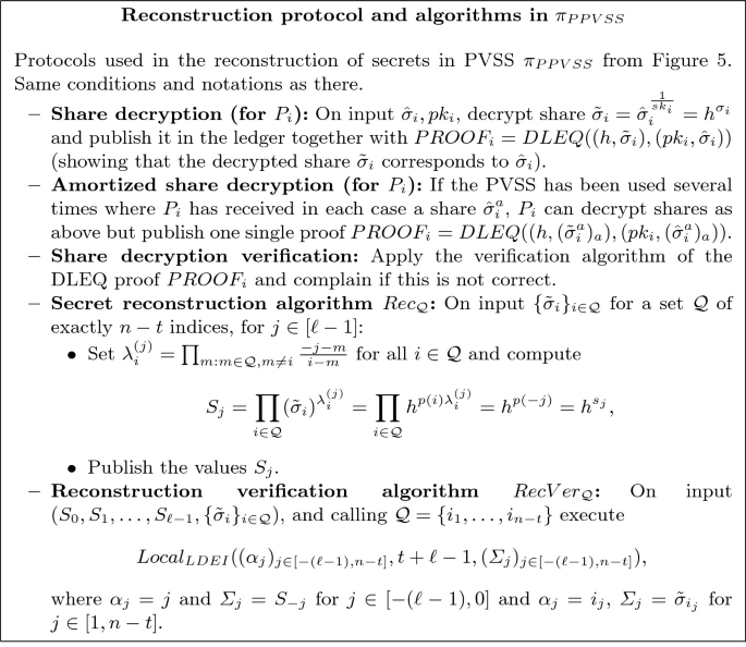
Reconstruction protocols and algorithms in $\pi _{PPVSS}$

We remark that the most expensive computation is reconstruction of a secret which requires $O(n^2)$ exponentiations.

4.2 Scheduling of Non-private Computations

In ALBATROSS, parties may need to carry out a number of computations of the form $M\diamond \mathbf {h}$, where $M\in \mathbb {Z}_q^{r\times m}$, $\mathbf {h}\in \mathbb {G}_q^m$ for some $r,m=O(n)$. This occurs if parties decide not to reveal their PVSSed secrets, and it happens at two moments of the computation: when reconstructing the secrets from the PVSS and when applying the resilient function at the output phase of the protocol.

These computations do not involve private information but especially in the PVSS they are expensive, requiring $O(n^2)$ exponentiations. Applying a resilient function via our $FFTE$ algorithm is considerably cheaper (it requires $O(n\log n)$ exponentiations), but depending on the application it still may make sense to apply the distributed computation techniques we are going to introduce.

On the other hand, given a purported output for such a computation, verifying their correctness can be done locally in a cheaper way (O(n) exponentiations) using respectively the tests $Local_{LDEI}$ for verifying PVSS reconstruction and a similar test which we call $Local_{LExp}$ for verifying the correct application of $FFTE$ (since we will not strictly need $Local_{LExp}$, we will not describe it here but it can be found in the full version of our paper).

In the worst case where $\varTheta (n)$ parties abort after having correctly PVSSed their secrets, $\varTheta (n)$ computations of each type need to be carried out. We balance the computational complexity of the parties as follows: for each of the tasks $\texttt {task}_i$ to be computed, a random set of computing parties $A_i$ is chosen of cardinality around some fixed value $c(n)$, who independently compute the task and publish their claimed outputs; the remaining parties verify which one of the outputs is correct, and if none of them is, they compute the tasks themselves.

Remark 4

The choice of $A_i$ has no consequences for the correctness and security of our protocols. The adversary may at most slow down the computation if it can arrange too many sets $A_i$ to contain no honest parties, but this requires a considerable amount of biasing of the randomness source. We will derive this randomness using a random oracle applied to the transcript of the protocol up to that moment, and assume for simplicity that each party has probability roughly $c(n)/n$ to belong to each $A_i$.

Let $\mathcal {T}=\{\texttt {task}_1,...,\texttt {task}_{f(n)}\}$ be a set of computation tasks, each of which consists of applying the same algorithm $AlgComp$ to an input $\texttt {in}_i$. Likewise, let $AlgVer$ be a verifying algorithm that given an input $\texttt {in}$ and a purported output $\texttt {out}$ always accepts if the output is correct and rejects it with very large probability if it is incorrect. We apply the protocol in Fig. 7.

Computational Complexity. We assume that $|\mathcal {P}|=\varTheta (n)$, and that $AlgComp$ requires $\texttt {ccost}(n)$ group exponentiations while $AlgVer$ needs $\texttt {vcost}(n)$. On expectation, each party will participate as computing party for $O(f(n)\cdot c(n)/n)$ tasks and as verifier for the rest, in each case needing to verify at most $c(n)$ computations. Note that we schedule the verifications so that parties check first the most common claimed output, as this will likely be the correct one. For a given $\texttt {task}_i$, if $A_i$ contains at least one honest party, then one of the verifications will be correct. $A_i$ contains only corrupt parties with probability $\tau ^{c(n)}$ where $\tau =t/n$ and therefore we can assume that the number of i’s for which this happens will be at most $O(\tau ^{c(n)}f(n))$, so parties will need to additionally apply $AlgComp$ on this number of tasks. Therefore the number of exponentiations per party is $\texttt {ccost}(n)\cdot O(( c(n)/n+\tau ^{c(n)})\cdot f(n))+\texttt {vcost}(n)\cdot O\left( c(n)\cdot \left( 1-c(n)/ n\right) \cdot f(n)\right) .$

Fig. 7.

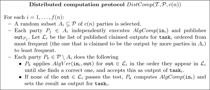
Distributed computation protocol $DistComp(\mathcal {T}, \mathcal {P}, c(n))$

PVSS Reconstruction. In the case of reconstruction of the PVSS’ed values, we have $AlgComp=Rec$ (Fig. 6), which has complexity $\texttt {ccost}(n)=O(n^2)$ and $AlgVer$ is $RecVer$ where $\texttt {vcost}(n)=O(n)$. The number of computations $f(n)$ equals the number of corrupted parties that correctly share a secret but later decide not to reveal it. In the worst case $f(n)=\varTheta (n)$. In that case, setting $c(n)=\log n$ gives a computational complexity of $O(n^2\log n)$ exponentiations. In fact the selection $c(n)=\log n$ is preferable unless $f(n)$ is small $(f(n)=O(\log n))$ where $c(n)=n$ (everybody reconstructs the $f(n)$ computations independently) is a better choice. For the sake of simplicity we will use $c(n)=\log n$ in the description of the protocols.

Output Reconstruction via $FFTE$. For this case we always have $f(n)=\ell =\varTheta (n)$. We use $FFTE$ as $AlgComp$, so $\texttt {ccost}(n)=O(n\log n)$, while $AlgVer$ is $Local_{LExp}$ where $\texttt {vcost}(n)=O(n)$. Setting $c(n)=|\mathcal {P}|$, $c(n)=\log n$ or $c(n)=\varTheta (1)$ all give $O(n^2\log n)$ exponentiations in the worst case.

Setting $c(n)=\varTheta (1)$ (a small constant number of parties computes each task, the rest verify) has a better best case asymptotic complexity: if every party acts honestly each party needs $O(n^2)$ exponentiations.

On the other hand, $c(n)=|\mathcal {P}|$ corresponds to every party carrying out the output computation by herself, so we do not really need $DistComp$ (and hence neither do we need $Local_{LExp}$). This requires less use of the ledger and a smaller round complexity, as the output of the majority is guaranteed to be correct. Moreover the practical complexity of $FFTE$ is very good, so in practice this option is computationally fast. We henceforth prefer this option, and leave $c(n)=\varTheta (1)$ as an alternative.

4.3 The ALBATROSS Multiparty Randomness Generation Algorithm

Next we present our randomness generation protocol ALBATROSS. We first introduce the following notation for having a matrix act on a matrix of group elements, by being applied to the matrix formed by their exponents.

Definition 5

As above, let $\mathbb {G}_q$ be a group of order q, and $h$ be a generator. Given a matrix $A=(A_{ij})$ in $\mathbb {Z}_q^{m_1\times m_2}$ and a matrix $B=(B_{ij})\in \mathbb {G}_q^{m_2\times m_3}$, we define $C=A\diamond B\in \mathbb {G}_q^{m_1\times m_3}$ with entries $C_{ij}=\prod _{k=1}^{m_2} B_{kj}^{A_{ik}}$.

Remark 5

An alternative way to write this is $C=h^{A\cdot D}$, where D in $\mathbb {Z}_q^{m_2\times m_3}$ is the matrix containing the discrete logs (in base h) of B, i.e. $D_{ij}=DLog_h(B_{ij})$. But we remark that we do not need to know D to compute C.

The protocol can be found in Fig. 8 and Fig. 9. In Fig. 8 we detail the first two phases Commit and Reveal: in the Commit phase the parties share random tuples $(h^{s_0^a},\dots ,h^{s_{\ell -1}^a})$ and prove correctness of the sharing. In the Reveal phase parties first verify correctness of other sharings. Once $n-t$ correct sharings have been posted,² the set $\mathcal {C}$ of parties that successfully posted correct sharings now open the sharing polynomials. The remaining parties verify this is consistent with the encrypted shares. If all parties in $\mathcal {C}$ open secrets correctly, then all parties learn the exponents $s_i^a$ and compute the final output by applying the resilient function in a very efficient manner, as explained in Fig. 9, step 4’.

If some parties do not correctly open their secret tuples, the remaining parties will use the PVSS reconstruction routine to retrieve the values $h^{s_j^a}$, and then compute the final output from the reconstructed values, now computing the resilient functions in the exponent. This is explained in Fig. 9.

Note that once a party gets into the set $\mathcal {C}$, her PVSS is correct (with overwhelming probability) and her tuple of secrets will be used in the final output, no matter the behaviour of that party from that point on. This is important: it prevents that the adversary biases the final randomness by initially playing honestly so that corrupted parties get into $\mathcal {C}$, and at that point deciding whether or not to open the secrets of each corrupted party conditioned on what other parties open. The fact that the honest parties can reconstruct the secrets from any party in $\mathcal {C}$ makes this behaviour useless to bias the output. On the other hand, the properties of the resilient function prevent the corrupted parties from biasing the output before knowing the honest parties’ inputs.

Theorem 2

With overwhelming probability, the protocol $\varPi _{ALB}$ has guaranteed output delivery and outputs a tuple of elements uniformly distributed in $\mathbb {G}_q^{\ell ^2}$, as long as the active, static, computationally bounded adversary corrupts at most t parties (where $2t+\ell =n$).

Proof

This theorem is based on the remarks above and formally proven in the full version of this paper  [13].

Fig. 8.

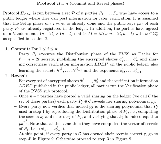
Protocol $\varPi _{ALB}$ (commit and reveal phases)

Fig. 9.

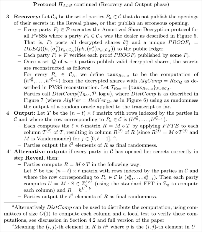
Protocol $\varPi _{ALB}$ continued

Computational Complexity: Group Exponentiations. In Table 1 we collect the complexity of ALBATROSS in terms of number of group exponentiations per party, comparing it with the SCRAPE protocol, where for ALBATROSS we assume $\ell =\varTheta (n)$. For the figures in the table, we consider both the worst case where $\varTheta (n)$ parties in $\mathcal {C}$ do not open their secrets in the Reveal phase, and the best case where all the parties open their secrets. As we can see the amortized cost for generating a random group element goes down from $O(n^2)$ exponentiations to $O(\log n)$ in the first case and O(1) in the second.

More in detail, in the Commit phase, both sharing a tuple of $\ell$ elements in the group costs O(n) exponentiations and proving their correctness take O(n) exponentiations. The Reveal phase takes $O(n^2)$ exponentiations since every party checks the $LDEI$ proofs of O(n) parties, each costing O(n) exponentiations, and similarly they later execute, for every party that reveals their sharing polynomial, O(n) exponentiations to check that this is consistent with the encrypted shares.

In the worst case O(n) parties from $\mathcal {C}$ do not open their secrets. The Recovery phase requires each then $O(n^2\log n)$ exponentiations per party, as explained in Sect. 4.2. The Output phase also requires $O(n^2\log n)$ exponentiations since $FFTE$ is used O(n) times (or if the alternative distributed technique is used, the complexity is also $O(n^2\log n)$ by the discussion in Sect. 4.2.

In the best case, all parties from $\mathcal {C}$ reveal their sharing polynomials correctly, the Recovery phase is not necessary and the Output phase requires $O(n^2)$ exponentiations per party as parties can compute the result directly by reconstructing the exponents first (where in addition one can use the standard FFT in $\mathbb {Z}_q$).

Computational Complexity: Other Operations. The total number of additional computation of group operations (aside from the ones involved in computing group exponentiations) is $O(n^2 \log n)$. With regard to operations in the field $\mathbb {Z}_q$, parties need to carry out a total of O(n) computations of polynomials of degree O(n) in sets of O(n) points, which are always subsets of the evaluation points for the secrets and share. In order to speed this computation up we can use $2n-th$ roots of unity as evaluation points (instead of $[-\ell -1,n]$) and make use of the FFT yielding a total of $O(n^2\log n)$ basic operations in $\mathbb {Z}_q$. We also need to compute Lagrange coefficients and the values $u_i$ in $Local_{LDEI}$ but this is done only once per party. In addition, the recent article [34] has presented efficient algorithms for all these computations.

Table 1. Computational complexity in terms of numbers of exponentiations for each phase of the protocols, and exponentiations per created element (per party).

Smaller Outputs. ALBATROSS outputs $O(n^2)$ random elements in the group $\mathbb {G}_q$. However, if parties do not need such large output, the protocol can be adapted to have a smaller output and a decreased complexity (even though the amortized complexity will be worse than the full ALBATROSS). In fact there are a couple of alternatives to achieve this: The first is to use standard (i.e., “non-packed” Shamir’s secret sharing, so a single group element is shared per party, as in SCRAPE; yet the resilient function based technique is still used to achieve an output of O(n) (assuming $t=(1/2-\epsilon ) n$). This yields a total computational complexity per party of $O(n^2)$ exponentiations (O(n) per output). A similar alternative is to instead use ALBATROSS as presented until the Recovery phase, and then only a subset $I\subset [0,\ell -1]$ of the coordinates of the secret vectors is used to construct a smaller output, and the rest is ignored. Then parties only need to recover those coordinates and apply the output phase to them. The advantage is that at a later point the remaining unused coordinates can be used on demand, if more randomness is needed (however it is important to note this unused randomness can not be considered secret anymore at this point, as it is computable from the information available to every party). If initially only O(n) random elements are needed, we set $|I|=O(1)$ and need $O(n^2)$ exponentiations per party (O(n) per output). We give more details in the full version.

Implementation. A toy implementation of some of the algorithms used in ALBATROSS can be found in [27].

5 Making ALBATROSS Universally Composable

In the previous sections, we constructed a packed PVSS scheme $\pi _{PPVSS}$ and used it to construct a guaranteed output delivery (G.O.D.) randomness beacon $\varPi _{ALB}$. However, as in previous G.O.D. unbiasable randomness beacons  [12, 23], we only argue stand alone security for this protocol. In the remainder of this work, we show that $\varPi _{ALB}$ can be lifted to achieve Universally Composability by two different approaches: 1. using UC-secure zero knowledge proofs of knowledge for the LDEI and DLEQ relations defined above, and 2. using UC-secure additively homomorphic commitments. We describe the UC framework, ideal functionalities and additional modelling details in the full version  [13].

Modeling Randomness Beacons in UC. We are interested in realizing a publicly verifiable G.O.D. coin tossing ideal functionality that functions as a randomness beacon (i.e. it allows any third party verifier to check whether a given output was previously generated by the functionality). We define such a functionality $\mathcal {F}_{\mathsf {CT}}^{m,\mathcal {D}}$ in Fig. 10. Notice that it provides random outputs once all honest parties activate it with independently from dishonest parties’ behavior. We realize this simple functionality for single shot coin tossing because it allows us to focus on the main aspects of our techniques. In order to obtain a stream of random values as in a traditional beacon, all parties can periodically call this functionality with a fresh sid.

Fig. 10.

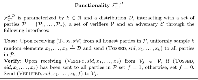
Functionality $\mathcal {F}_{\mathsf {CT}}^{k,\mathcal {D}}$ for G.O.D. publicly verifiable coin tossing.

5.1 Using UC-Secure Zero Knowledge Proofs

Our first approach is to modify the commit and reveal phases of Protocol $\varPi _{ALB}$ and use NIZK ideal functionalities as setup (along with an authenticated public bulletin board ideal functionality $\mathcal {F}_{APBB}$ as defined in the full version  [13]) in order to obtain an UC-secure version of protocol. The crucial difference is that instead of having all parties reveal the randomness of the PVSS sharing algorithm (i.e. the polynomial p(X)) in the reveal phase in order to verify that certain random inputs were previously shared in the commit phase, we have the parties commit to their random inputs using an equivocal commitment and then generate a NIZK proof that the random inputs in the commitments correspond to the ones shared by the PVSS scheme in the commit phase. In the reveal phase, the parties simply open their commitments. In case a commitment is not opened, the honest parties use the PVSS reconstruction to recover the random input. Intuitively, using an equivocal commitment scheme and ideal NIZKs allows the simulator to first extract all the random inputs shared by the adversary and later equivocate the simulated parties’ commitment openings in order to trick the adversary into accepting arbitrary random inputs from simulated honest parties that result in the same randomness as obtained from $\mathcal {F}_{\mathsf {CT}}$. Protocol $\varPi _{CT-ZK}$ is presented in Figs. 11 and 12.

Pedersen Commitments. We will use a Pedersen commitment  [28], which is an equivocal commitment, i.e. it allows a simulator who knows a trapdoor to open a commitment to any arbitrary message. In this scheme, all parties are assumed to know generators g, h of a group $\mathbb {G}_q$ of prime order q chosen uniformly at random such that the discrete logarithm of h on base g is unknown. In order to commit to a message $m \in \mathbb {Z}_q$, a sender samples a randomness $r \, {\mathop {\leftarrow }\limits ^{{\scriptscriptstyle \$}}}\, \mathbb {Z}_q$ and computes a commitment $c=g^m h^r$, which can be later opened by revealing (m, r). In order to verify that an opening $(m',r')$ for a commitment c is valid, a receiver simply checks that $c=g^{m'} h^{r'}$. However, a simulator who knows a trapdoor $\mathsf {td}$ such that $h=g^{\mathsf {td}}$ can open $c=g^m h^r$ to any arbitrary message $m'$ by computing $r'=\frac{m+\mathsf {td}\cdot r-m'}{\mathsf {td}}$ and revealing $(m',r')$. For a message $m \in \mathbb {Z}_q$ and randomness $r \in \mathbb {Z}_q$, we denote a commitment c as $\mathsf {Com}(m,r)$, the opening of c as $\mathsf {Open}(m,r)$ and the opening of c to an arbitrary message $m' \in \mathbb {Z}_q$ given trapdoor $\mathsf {td}$ as $\mathsf {TDOpen}(m,r,m',\mathsf {td})$.

Fig. 11.

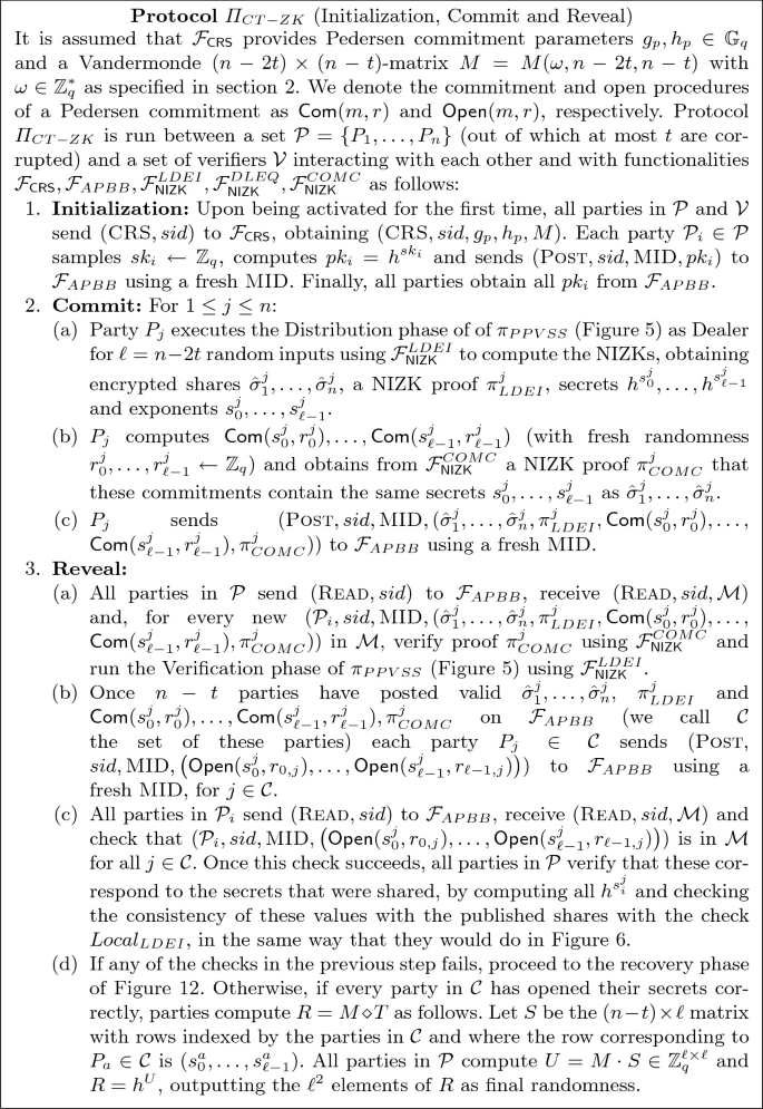
Protocol $\varPi _{CT-ZK}$, optimistic case (initialization, commit and reveal).

Fig. 12.

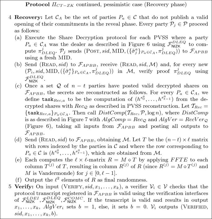
Protocol $\varPi _{CT-ZK}$ continued, pessimistic case (recovery phase)

NIZKs. We use three instances of functionality $\mathcal {F}^{R}_{\mathsf {NIZK}}$. The first one is $\mathcal {F}^{LDEI}_{\mathsf {NIZK}}$, which is parameterized with relation $LDEI$ (Sect. 3). The second one is $\mathcal {F}^{DLEQ}_{\mathsf {NIZK}}$, which is parameterized with relation DLEQ for multiple statements $DLEQ((h,(\tilde{\sigma }^i_j)_{i \in I})(pk,(\hat{\sigma }_j^i)_{i \in I}))$ (Sect. 3). The third and final one is $\mathcal {F}^{COMC}_{\mathsf {NIZK}}$, which is parameterized with a relation $COMC$ showing that commitments $\mathsf {Com}(s_0^j,r_0^j), \ldots ,\mathsf {Com}(s_{\ell -1}^j,r_{\ell -1}^j)$ contain the same secrets $s_0^j,\ldots ,s_{\ell -1}^j$ as in the encrypted shares $\hat{\sigma }^j_1,\ldots ,\hat{\sigma }^j_n$ generated by $\pi _{PPVSS}$ (Fig. 5).

CRS and Bulletin Board. In order to simplify our protocol description and security analysis, we assume that parties have access to a CRS containing the public parameters for the Pedersen equivocal commitment scheme and Vandermonde matrix for the PVSS scheme $\pi _{PPVSS}$. Moreover, a CRS would be necessary to realize the instances of $\mathcal {F}^{R}_{\mathsf {NIZK}}$ we use. Nevertheless, we remark that the parties could generate all of these values in a publicly verifiable way through a multiparty computation protocol  [7] and register them in the authenticated public bulletin board functionality in the beginning of the protocol.

Communication Model. Formally, for the sake of simplicity, we describe our protocol using an ideal authenticated public bulletin board $\mathcal {F}_{APBB}$ that guarantees all messages appear immediately in the order they are received and become immutable. However, we remark that our protocols can be proven secure in a semi-synchronous communication model with a public ledger where messages are arbitrarily delayed and re-ordered by the adversary but eventually registered (i.e. the adversary cannot drop messages or induce an infinite delay). Notice that the protocol proceeds to each of its steps once $n-t$ parties (i.e. at least all honest parties) post their messages to $\mathcal {F}_{APBB}$, so it is guaranteed to terminate if honest party messages are delivered eventually regardless of the order in which these messages appear or of the delay for such messages to become immutable. Using the terminology of  [3, 21], if we were to use a blockchain based public ledger instead of $\mathcal {F}_{APBB}$, each point we state that the parties wait for $n-t$ valid messages to be posted to $\mathcal {F}_{APBB}$ could be adapted to having the parties wait for enough rounds such that it is guaranteed by the chain growth property that a large number enough blocks are added to the ledger in such a way that the chain quality property guarantees that at least one of these blocks is honest (i.e. containing honest party messages) and that enough blocks are guaranteed to be added after this honest block so that the common prefix property guarantees that all honest parties have this block in their local view of the ledger. A similar analysis has been done in  [18, 23] in their constructions of randomness beacons.

Complexity. We execute essentially the same steps of Protocol $\varPi _{ALB}$ with the added overhead of having each party compute Pedersen Commitments to their secrets and generate a NIZK showing these secrets are the same as the ones shared through the PVSS scheme. Using the combined approaches of  [9, 24] to obtain these NIZKs, the approximate extra overhead of using UC NIZKs in relation to the stand alone NIZKs of $\varPi _{ALB}$ will be that of computing 2 evaluations of the Paillier cryptosystem’s homomorphism and 4 modular exponentiations over $\mathbb {G}_q$ per each secret value in the witness for each NIZK. In the Commit and Reveal phases, this yields an approximate fixed extra cost of $4n^2$ evaluations of the Paillier cryptosystem’s homomorphism and $8n^2$ modular exponentiations over $\mathbb {G}_q$ for generating and verifying NIZKs with $\mathcal {F}^{LDEI}_{\mathsf {NIZK}}$ and $\mathcal {F}^{COMC}_{\mathsf {NIZK}}$. In the recovery phase, if a parties fail to open their commitments, there is an extra costs of $2a(n-t)$ evaluations of the Paillier cryptosystem’s homomorphism and $4a(n-t)$ modular exponentiations over $\mathbb {G}_q$ for generating and verifying NIZKs with $\mathcal {F}^{DLEQ}_{\mathsf {NIZK}}$. In terms of communication, the approximate extra overhead is of one Paillier ciphertext and two integer commitments per each secret value in the witness for each NIZK, yielding an approximate total overhead of $(n^2+a(n-t)) \cdot |\mathsf {Paillier}|+(2n^2+a(n-t))\cdot |\mathbb {G}_q|$ bits where $|\mathsf {Paillier}|$ is the length of a Paillier ciphertext and $|\mathbb {G}_q|$ is the length of a $\mathbb {G}_q$ element.

Theorem 3

Protocol $\varPi _{CT-ZK}$ UC-realizes $\mathcal {F}_{\mathsf {CT}}^{k,\mathcal {D}}$ for $k=\ell ^2=(n-2t)^2$ and $\mathcal {D}= \{h^{s} | h \in \mathbb {G}_q, s \, {\mathop {\leftarrow }\limits ^{{\scriptscriptstyle \$}}}\, \mathbb {Z}_q \}$ in the $\mathcal {F}_{\mathsf {CRS}},\mathcal {F}_{APBB},\mathcal {F}^{LDEI}_{\mathsf {NIZK}},\mathcal {F}^{DLEQ}_{\mathsf {NIZK}},\mathcal {F}^{COMC}_{\mathsf {NIZK}}$-hybrid model with static security against an active adversary $\mathcal {A}$ corrupting corrupts at most t parties (where $2t+\ell =n$) parties under the DDH assumption.

Proof

We prove this theorem in the full version  [13].

5.2 Using Designated Verifier Homomorphic Commitments

In the stand alone version of ALBATROSS and the first UC-secure version we construct, the main idea is to encrypt shares of random secrets obtained from packed Shamir secret sharing and prove in zero knowledge that those shares were consistently generated. Later on, zero knowledge proofs are used again to prove that decrypted were correctly obtained from the ciphertexts that have already been verified for consistency, ensuring secrets can be properly reconstructed. We now explore an alternative where we instead commit to their shares using a UC additively homomorphic commitment scheme and perform a version the $Local_{LDEI}$ check on the committed shares and open the resulting commitment in order to prove that their shares were correctly generated. In order to do that, we need a new notion of a UC additively homomorphic commitment that allows for the sender to open a commitments to an specific share towards a specific party (so that only that party learns its share) but allows for those parties to later prove that they have received a valid opening or not, allowing the other parties to reconstruct the secrets from the opened shares. In the remainder of this section, we introduce our new definition of such a commitment scheme and show how it can be used along with $\mathcal {F}_{APBB}$ to realize $\mathcal {F}_{\mathsf {CT}}^{k,\mathcal {D}}$.

Fig. 13.

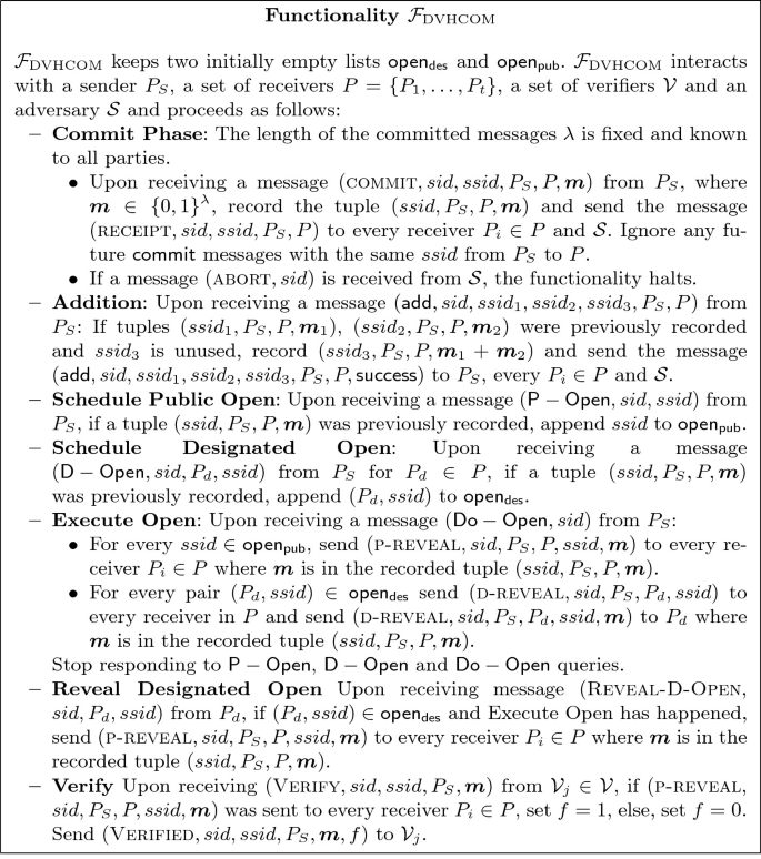
Functionality $\mathcal {F}_\mathrm {DVHCOM}$

Designated Verifier Commitments. We define a new flavor of multi-receiver commitments that we call Designated Verifier Commitments, meaning that they allow a sender to open a certain commitment only towards a certain receiver in such a way that this receiver can later prove that the commitment was correctly opened (also revealing its message) or that the opening was not valid. Moreover, we give this commitments the ability to evaluate linear functions on committed values and reveal only the result of these evaluations but not the individual values used as input, a property that is called additive homomorphism. We depart from the multi-receiver additively homomorphic commitment functionality from  [11] and augment it with designated verifier opening and verification interfaces. Functionality $\mathcal {F}_\mathrm {DVHCOM}$ is presented in Fig. 13. The basic idea to realize this functionality is that we make two important changes to the protocol of  [11]: 1. all protocol messages are posted to the authenticated bulletin board $\mathcal {F}_{APBB}$; 2. designated openings are done by encrypting the opening information from the protocol of  [11] with the designated verifier’s public key for a cryptosystem with plaintext verification  [4], which allows the designated verifier to later publicly prove that a certain (in)valid commitment opening was in the ciphertext. Interestingly, $\mathcal {F}_\mathrm {DVHCOM}$ can be realized in the global random oracle model under the Computational Diffie Hellman (CDH) assumption. We show how to realize $\mathcal {F}_\mathrm {DVHCOM}$ in the full version  [13].

Fig. 14.

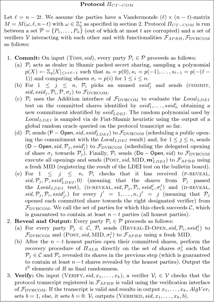
Protocol $\varPi _{CT-COM}$.

Realizing $\varvec{\mathcal {F}_{\mathsf {CT}}^{k,\mathcal {D}}}$ with $\varvec{\varPi _{CT-COM}}$ . The main idea in constructing Protocol $\varPi _{CT-COM}$ is to have each party compute shares of their random secrets using packed Shamir secret sharing and then generate designated verifier commitments $\mathcal {F}_\mathrm {DVHCOM}$ to each share. Next, each party proves that their committed shares are valid by executing the $Local_{LDEI}$ test on the committed shares (instead of group exponents), which involves evaluating a linear function on the committed shares and publicly opening the commitment containing the result of this evaluation. At the same time, each party performs designated openings of each committed share towards one of the other parties, who verify that they have obtained a valid designated opening and post a message to $\mathcal {F}_{APBB}$ confirming that this check succeeded. After a high enough number of parties successfully confirms this check for each of the sets of committed shares, each party publicly opens all of their committed shares, allowing the other parties to reconstruct the secrets. If one of the parties does not open all of their shares, the honest parties can still reconstruct the secrets by revealing the designated openings they received for their shares. We present Protocol $\varPi _{CT-COM}$ in Fig. 14 and state its security in Theorem 4. Since $\mathcal {F}_\mathrm {DVHCOM}$ can be realized in the global random oracle model under the Computational Diffie Hellman (CDH) assumption as shown in the full version  [13], we obtain an instantiation of $\mathcal {F}_{\mathsf {CT}}^{k,\mathcal {D}}$ with security based on CDH.

Theorem 4

Protocol $\varPi _{CT-COM}$ UC-realizes $\mathcal {F}_{\mathsf {CT}}^{k,\mathcal {D}}$ for $k=\ell ^2=(n-2t)^2$ and $\mathcal {D}= \{h^{s} | h \in \mathbb {G}_q, s \, {\mathop {\leftarrow }\limits ^{{\scriptscriptstyle \$}}}\, \mathbb {Z}_q \}$ in the $\mathcal {F}_\mathrm {DVHCOM},\mathcal {F}_{APBB}$-hybrid model with static security against an active adversary $\mathcal {A}$ corrupting at most t parties (where $2t+\ell =n$).

Proof

This theorem is proven in the full version  [13].

References

Adida, B.: Helios: web-based open-audit voting. In: Proceedings of the 17th USENIX Security Symposium, pp. 335–348 (2008)
Azouvi, S., McCorry, P., Meiklejohn, S.: Winning the caucus race: continuous leader election via public randomness. CoRR, abs/1801.07965 (2018)
Badertscher, C., Maurer, U., Tschudi, D., Zikas, V.: Bitcoin as a transaction ledger: a composable treatment. In: Katz, J., Shacham, H. (eds.) CRYPTO 2017. LNCS, vol. 10401, pp. 324–356. Springer, Cham (2017). https://doi.org/10.1007/978-3-319-63688-7_11
Baum, C., David, B., Dowsley, R.: A framework for universally composable publicly verifiable cryptographic protocols. Cryptology ePrint Archive, Report 2020/207 (2020). https://eprint.iacr.org/2020/207
Blakley, G.R., Meadows, C.: Security of ramp schemes. In: Blakley, G.R., Chaum, D. (eds.) CRYPTO 1984. LNCS, vol. 196, pp. 242–268. Springer, Heidelberg (1985). https://doi.org/10.1007/3-540-39568-7_20
Boneh, D., Bonneau, J., Bünz, B., Fisch, B.: Verifiable delay functions. In: Shacham, H., Boldyreva, A. (eds.) CRYPTO 2018. LNCS, vol. 10991, pp. 757–788. Springer, Cham (2018). https://doi.org/10.1007/978-3-319-96884-1_25
Bowe, S., Gabizon, A., Green, M.D.: A multi-party protocol for constructing the public parameters of the Pinocchio zk-SNARK. In: Zohar, A., et al. (eds.) FC 2018. LNCS, vol. 10958, pp. 64–77. Springer, Heidelberg (2019). https://doi.org/10.1007/978-3-662-58820-8_5
Bowe, S., Grigg, J., Hopwood, D.: Halo: recursive proof composition without a trusted setup. IACR Cryptology ePrint Archive, 2019:1021 (2019)
Camenisch, J., Krenn, S., Shoup, V.: A framework for practical universally composable zero-knowledge protocols. In: Lee, D.H., Wang, X. (eds.) ASIACRYPT 2011. LNCS, vol. 7073, pp. 449–467. Springer, Heidelberg (2011). https://doi.org/10.1007/978-3-642-25385-0_24
Canetti, R.: Universally composable security: a new paradigm for cryptographic protocols. In: 42nd FOCS, pp. 136–145. IEEE Computer Society Press, October 2001
Cascudo, I., Damgård, I., David, B., Döttling, N., Dowsley, R., Giacomelli, I.: Efficient UC commitment extension with homomorphism for free (and applications). In: Galbraith, S.D., Moriai, S. (eds.) ASIACRYPT 2019, Part II. LNCS, vol. 11922, pp. 606–635. Springer, Cham (2019). https://doi.org/10.1007/978-3-030-34621-8_22
Cascudo, I., David, B.: SCRAPE: scalable randomness attested by public entities. In: Gollmann, D., Miyaji, A., Kikuchi, H. (eds.) ACNS 2017. LNCS, vol. 10355, pp. 537–556. Springer, Cham (2017). https://doi.org/10.1007/978-3-319-61204-1_27
Cascudo, I., David, B.: ALBATROSS: publicly attestable batched randomness based on secret sharing (full version). Cryptology ePrint Archive, Report 2020/644 (2020). https://eprint.iacr.org/2020/644
Chaum, D., Pedersen, T.P.: Wallet databases with observers. In: Brickell, E.F. (ed.) CRYPTO 1992. LNCS, vol. 740, pp. 89–105. Springer, Heidelberg (1993). https://doi.org/10.1007/3-540-48071-4_7
Chen, J., Micali, S.: Algorand: a secure and efficient distributed ledger. Theor. Comput. Sci. 777, 155–183 (2019)
Chor, B., Goldreich, O., Håstad, J., Friedman, J., Rudich, S., Smolensky, R.: The bit extraction problem of t-resilient functions. In: 26th Annual Symposium on Foundations of Computer Science, Portland, Oregon, USA, 21–23 October 1985, pp. 396–407 (1985)
Cooley, J.W., Tukey, J.W.: An algorithm for the machine calculation of complex Fourier series. Math. Comp. 19, 297–301 (1965)
David, B., Gaži, P., Kiayias, A., Russell, A.: Ouroboros Praos: an adaptively-secure, semi-synchronous proof-of-stake blockchain. In: Nielsen, J.B., Rijmen, V. (eds.) EUROCRYPT 2018. LNCS, vol. 10821, pp. 66–98. Springer, Cham (2018). https://doi.org/10.1007/978-3-319-78375-8_3
Fiat, A., Shamir, A.: How to prove yourself: practical solutions to identification and signature problems. In: Odlyzko, A.M. (ed.) CRYPTO 1986. LNCS, vol. 263, pp. 186–194. Springer, Heidelberg (1987). https://doi.org/10.1007/3-540-47721-7_12
Franklin, M.K., Yung, M.: Communication complexity of secure computation (extended abstract). In: Proceedings of the 24th Annual ACM Symposium on Theory of Computing, Victoria, British Columbia, Canada, 4–6 May 1992, pp. 699–710 (1992)
Garay, J., Kiayias, A., Leonardos, N.: The bitcoin backbone protocol: analysis and applications. In: Oswald, E., Fischlin, M. (eds.) EUROCRYPT 2015, Part II. LNCS, vol. 9057, pp. 281–310. Springer, Heidelberg (2015). https://doi.org/10.1007/978-3-662-46803-6_10
Heidarvand, S., Villar, J.L.: Public verifiability from pairings in secret sharing schemes. In: Avanzi, R.M., Keliher, L., Sica, F. (eds.) SAC 2008. LNCS, vol. 5381, pp. 294–308. Springer, Heidelberg (2009). https://doi.org/10.1007/978-3-642-04159-4_19
Kiayias, A., Russell, A., David, B., Oliynykov, R.: Ouroboros: a provably secure proof-of-stake blockchain protocol. In: Katz, J., Shacham, H. (eds.) CRYPTO 2017. LNCS, vol. 10401, pp. 357–388. Springer, Cham (2017). https://doi.org/10.1007/978-3-319-63688-7_12
Lindell, Y.: An efficient transform from sigma protocols to NIZK with a CRS and non-programmable random oracle. In: Dodis, Y., Nielsen, J.B. (eds.) TCC 2015, Part I. LNCS, vol. 9014, pp. 93–109. Springer, Heidelberg (2015). https://doi.org/10.1007/978-3-662-46494-6_5
Nakamoto, S.: Bitcoin: a peer-to-peer electronic cash system. Manuscript (2008). https://bitcoin.org/bitcoin.pdf
Naor, M., Reingold, O.: Number-theoretic constructions of efficient pseudo-random functions. J. ACM 51(2), 231–262 (2004)
Palandjian, E.: Implementation of ALBATROSS. https://github.com/evapln/albatross
Pedersen, T.P.: Non-interactive and information-theoretic secure verifiable secret sharing. In: Feigenbaum, J. (ed.) CRYPTO 1991. LNCS, vol. 576, pp. 129–140. Springer, Heidelberg (1992). https://doi.org/10.1007/3-540-46766-1_9
Pointcheval, D., Stern, J.: Security proofs for signature schemes. In: Maurer, U. (ed.) EUROCRYPT 1996. LNCS, vol. 1070, pp. 387–398. Springer, Heidelberg (1996). https://doi.org/10.1007/3-540-68339-9_33
Rabin, M.O.: Transaction protection by beacons. J. Comput. Syst. Sci. 27(2), 256–267 (1983)
Ruiz, A., Villar, J.L.: Publicly verfiable secret sharing from Paillier’s cryptosystem. In: WEWoRC 2005, pp. 98–108 (2005)
Shamir, A.: How to share a secret. Commun. ACM 22(11), 612–613 (1979)
Syta, E., et al.: Scalable bias-resistant distributed randomness. In: 2017 IEEE Symposium on Security and Privacy, SP 2017, pp. 444–460 (2017)
Tomescu, A., et al.: Towards scalable threshold cryptosystems. In: IEEE Symposium on Security and Privacy, pp. 1367–1383 (2020)
van den Hooff, J., Lazar, D., Zaharia, M., Zeldovich, N.: Vuvuzela: scalable private messaging resistant to traffic analysis. In: Proceedings of the 25th Symposium on Operating Systems Principles, SOSP 2015, pp. 137–152 (2015)
Wolinsky, D.I., Corrigan-Gibbs, H., Ford, B., Johnson, A.: Dissent in numbers: making strong anonymity scale. In: Proceedings of the 10th USENIX Conference on Operating Systems Design and Implementation, OSDI 2012, pp. 179–192 (2012)
Acknowledgements
The authors would like to thank the anonymous reviewers for their suggestions, Diego Aranha, Ronald Cramer and Dario Fiore for useful discussions and Eva Palandjian for the implementation in [27] and remarks about the initial draft.
Author information
Authors and Affiliations
Corresponding author
Editor information
Editors and Affiliations
Rights and permissions
Copyright information
© 2020 International Association for Cryptologic Research
About this paper
Cite this paper
Cascudo, I., David, B. (2020). ALBATROSS: Publicly AttestabLe BATched Randomness Based On Secret Sharing. In: Moriai, S., Wang, H. (eds) Advances in Cryptology – ASIACRYPT 2020. ASIACRYPT 2020. Lecture Notes in Computer Science(), vol 12493. Springer, Cham. https://doi.org/10.1007/978-3-030-64840-4_11
Download citation
DOI: https://doi.org/10.1007/978-3-030-64840-4_11
Published:
Publisher Name: Springer, Cham
Print ISBN: 978-3-030-64839-8
Online ISBN: 978-3-030-64840-4
eBook Packages: Computer ScienceComputer Science (R0)