Constant-Size Structure-Preserving Signatures: Generic Constructions and Simple Assumptions

Abstract

This paper presents efficient structure-preserving signature schemes based on simple assumptions such as decisional linear. We first give two general frameworks for constructing fully secure signature schemes from weaker building blocks such as variations of one-time signatures and random message secure signatures. They can be seen as refinements of the Even–Goldreich–Micali framework, and preserve many desirable properties of the underlying schemes such as constant signature size and structure preservation. We then instantiate them based on simple (i.e., not q-type) assumptions over symmetric and asymmetric bilinear groups. The resulting schemes are structure-preserving and yield constant-size signatures consisting of 11–14 group elements, which compares favorably to existing schemes whose security relies on q-type assumptions.

1 Introduction

A structure-preserving signature (SPS) scheme [4] is a digital signature scheme with two structural properties: (1) the verification keys, messages, and signatures are all elements of a bilinear group; and (2) the verification algorithm checks a conjunction of pairing product equations over the key, the message, and the signature. This makes them compatible with the efficient non-interactive proof system for pairing product equations by Groth and Sahai (GS) [33]. Structure-preserving cryptographic primitives promise to combine the advantages of optimized number theoretic non-black-box constructions with the modularity and insight into protocols that use only generic cryptographic building blocks.

Indeed the instantiation of known generic constructions with an SPS scheme and the GS proof system has led to many new and more efficient schemes: Groth [32] showed how to construct an efficient simulation-sound zero-knowledge proof system (ss-NIZK) building on generic constructions of [20, 37, 41]. Abe et al. [4, 7] show how to obtain efficient round-optimal blind signatures by instantiating a framework by Fischlin [23]. SPS are also important building blocks for a wide range of cryptographic functionalities such as anonymous proxy signatures [25], delegatable anonymous credentials [9], transferable e-cash [26] and compact verifiable shuffles [18]. Most recently, Hofheinz and Jager [34] show how to construct a structure- preserving tree-based signature scheme with a tight security reduction following the approach of [21, 29]. This signature scheme is then used to build a ss-NIZK which in turn is used with the Naor and Yung [38] and Sahai [40] paradigm to build the first CCA-secure public-key encryption scheme with a tight security reduction. Examples for other schemes that benefit from efficient SPS are [8, 10, 11, 14, 24, 27, 30, 31, 35, 39].

Because properties (1) and (2) are the only dependencies on the SPS scheme made by these constructions, any structure-preserving signature scheme can be used as a drop-in replacement. Unfortunately, all known efficient instantiations of SPS [4, 5, 7] are based on so-called q-type or interactive assumptions. An open question since Groth’s seminal work [32] (only partially answered by Chase and Kohlweiss [17]) is to construct a SPS scheme that is both efficient—in particular constant-size in the number of signed group elements—and that is based on assumptions that are as weak as those required by the GS proof system itself.

1.1 Our Contribution

We begin by presenting two new generic constructions of signature schemes that are secure against chosen message attacks (CMA) from variations of one-time signatures and signatures secure against random message attacks (RMA). Both constructions inherit the structure-preserving and constant-size properties from the underlying components. We then instantiate the building blocks with the desired properties over bilinear groups. They yield constant-size structure-preserving signature schemes whose signatures consist of only 11–14 group elements and whose security can be proven based on simple assumptions such as decisional linear ($\text {DLIN}$) for symmetric bilinear groups and analogues of DDH and $\text {DLIN}$ for asymmetric bilinear groups. These are the first constant-size structure-preserving signature schemes that eliminate the use of interactive or q-type assumptions while achieving reasonable efficiency. We give more details on our generic constructions and their instantiations:

• The first generic construction ($\mathsf {SIG{1}}$, Sect. 4.1) combines a new variation of one-time signatures which we call tagged one-time signatures ($\mathsf {TOS}$) and signatures secure against random message attacks (RMA). A $\mathsf {TOS}$ is a signature scheme that attaches a fresh tag to each signature. It is unforgeable with respect to tags used only once. In our construction, a message is signed with our $\mathsf {TOS}$ using a fresh random tag, and then the tag is signed with the second signature scheme, denoted by ${\mathsf {{r}SIG{}}}$. Since ${\mathsf {{r}SIG{}}}$ only signs random tags, RMA security is sufficient.

  In Sect. 5, we construct structure-preserving $\mathsf {TOS}$ and ${\mathsf {{r}SIG{}}}$ based on $\text {DLIN}$ over symmetric (Type-I) bilinear groups. Our $\mathsf {TOS}$ yields constant-size signatures and optimally small tags that consist of only one group element. The resulting structure-preserving signature scheme produces signatures consisting of 14 group elements, and relies solely on the $\text {DLIN}$ assumption.¹

• The second generic construction ($\mathsf {SIG{2}}$, Sect. 4.2) combines partial one-time signatures and signatures secure against extended random message attacks (XRMA). The latter is a new notion that we explain below. A partial one-time signature scheme, denoted by $\mathsf {POS}$, is a one-time signature scheme in which only a part of the key is renewed for every signing operation. The notion was first introduced by Bellare and Shoup [12] under the name of two-tier signatures. In our construction, a message is signed with $\mathsf {POS}$ and then the one-time portion of the public-key is certified by the second signature scheme, denoted by ${\mathsf {{x}SIG{}}}$. The difference between a $\mathsf {TOS}$ and $\mathsf {POS}$ is that a one-time public-key is associated with a one-time secret-key. Since the one-time secret-key is needed for signing, it must be known to the reduction in the security proof. XRMA security guarantees that ${\mathsf {{x}SIG{}}}$ is unforgeable even if the adversary is given auxiliary information associated with the randomly chosen messages (e.g. the random coins used for selecting the message). The auxiliary information allows the reduction algorithm of the security proof of the second scheme to use the one-time secret-key to generate the $\mathsf {POS}$ component correctly.

  In Sect. 6, we construct structure-preserving $\mathsf {POS}$ and ${\mathsf {{x}SIG{}}}$ signature schemes based on assumptions that are analogues of DDH and $\text {DLIN}$ in Type-III bilinear groups. The resulting ${\mathsf {SIG{2}}}$ is structure-preserving and produces signatures consisting of 11 or 14 group elements depending on whether messages belong to either or both source groups.

The role of $\mathsf {TOS}$ and $\mathsf {POS}$ is to compress a message into a constant number of random group elements. This observation is interesting in light of [6] that implies the impossibility of constructing collision resistant and shrinking structure-preserving hash functions, which could immediately yield constant-size signatures. Our (extended) RMA-secure signature schemes are structure-preserving variants of Waters’ dual-signature scheme [44]. In general, the difficulty of constructing CMA-secure SPS arises from the fact that the exponents of the group elements chosen by the adversary as a message are not known to the reduction in the security proof. On the other hand, for RMA security, it is the challenger that chooses the message and therefore the exponents can be known in reductions. This is the crucial advantage for constructing (extended) RMA-secure structure-preserving signature schemes based on Waters’ dual-signature scheme.

As our SPSs can be drop-in replacements for existing SPS, we only briefly introduce recent applications in Sect. 7. They include group signatures, tightly-secure structure-preserving signatures and public-key encryption, and efficient adaptive oblivious transfer.

1.2 Related Works

1.2.1 On Generic Constructions

Even et al. [22] proposed a generic framework (the EGM framework) that combines a one-time signature scheme and a signature scheme that is secure against non-adaptive chosen message attacks (NACMA) to construct a signature scheme that is secure against adaptive chosen message attacks (CMA).

In fact, our generic constructions can be seen as refinements of the EGM framework. There are two reasons why the original framework falls short for our purpose. The first is that relaxing to NACMA does not seem to help much in constructing efficient structure-preserving signatures since the messages are still under the control of the adversary, and the exponents of the messages are not known to the reduction algorithm in the security proof. As mentioned above, resorting to (extended) RMA is a great help in this regard. In [22], they also showed that CMA-secure signatures exist iff RMA-secure signatures exist. The proof, however, does not follow their framework and their impractical construction is mainly a feasibility result. In fact, we argue that RMA-security alone is not sufficient for the original EGM framework. As mentioned above, the necessity of $\text {XRMA}$ security arises in the reduction that uses $\text {RMA}$-security to argue security of the ordinary signature scheme, as the reduction not only needs to know the random one-time public-keys, but also their corresponding one-time secret-keys in order to generate the one-time signature components of the signatures. The auxiliary information in the $\text {XRMA}$ definition facilitates access to these secret-keys. Similarly, tagged one-time signatures avoid this problem as tags do not have associated secret values. This observation applies also to a variation of the EGM framework in [42] that combines a trapdoor hash function and a NACMA-secure signature scheme. The second reason that the EGM approach is not quite suited to our task is that the EGM framework produces signatures that are linear in the size of one-time public-keys of the one-time signature scheme, and known structure-preserving one-time signature schemes have one-time public-keys that scale linearly with the number of group elements to be signed. Here, tagged or partial one-time signature schemes come in handy as they have one-time public-keys separated from long-term public-keys. Thus, to obtain constant-size signatures, we only require the one-time keys to be constant-size while allowing the long-term part to scale in the size of the message.

1.2.2 On Efficient Instantiations

All previous constructions of structure-preserving signature schemes either are inefficient, or use strong assumptions, or do not yield constant-size signatures. In particular, there are few schemes that are based on simple assumptions. Hofheinz and Jager [34] constructed an SPS scheme by following the EGM framework. The resulting scheme allows a tight security reduction to $\text {DLIN}$, but the size of signatures depends logarithmically on the number of signing operations as their NACMA-secure scheme is tree-based (like the Goldwasser–Micali–Rivest signature scheme [29]). Chase and Kohlweiss [17] and Camenisch et al. [15] constructed SPS schemes with security based on $\text {DLIN}$ that improve the performance of Groth’s scheme [32] by several orders of magnitude. The size of the resulting signatures, however, is still linear in the number of signed group elements.

2 Preliminaries

2.1 Notation

By $X :=Y$, we denote that object Y is referred to as X. For set X, notation $a \leftarrow X$ denotes a uniform sampling from X. Multiple independent samples from the same set X are denoted by $a_1,a_2,a_3,\ldots \leftarrow X$. By $Y \leftarrow A(X)$, we denote the process where algorithm A is executed with X as input and its output is labeled as Y. When A is an oracle algorithm that interacts with oracle $\mathcal O$, it is denoted as $Y \leftarrow A^\mathcal{O}(X)$. By $\Pr [X \,|\, A_1, A_2, \ldots , A_k ]$ we denote the probability that event X happens after executing the sequence of algorithms $A_1, \ldots , A_k$. The probability is taken over all coin flips observed in $A_1,\ldots ,A_k$ unless otherwise noted. We say that a function $\epsilon$ is negligible in security parameter $\lambda$ if $\epsilon < \lambda ^{-c}$ holds for all constant $c>0$ and all sufficiently large $\lambda$. We refer to probabilistic polynomial- time algorithms as p.p.t. algorithms. Unless stated otherwise, we assume that all algorithms are potentially probabilistic.

2.2 Bilinear Groups

Let ${\mathcal {G}}$ be a bilinear group generator that takes security parameter $1^\lambda$ and outputs a description of bilinear groups $\varLambda :=(p,{{\mathbb G}}_1,{{\mathbb G}}_2,{{\mathbb G}}_T,e)$, where ${{\mathbb G}}_1,\,{{\mathbb G}}_2$ and ${{\mathbb G}}_T$ are groups of prime order $p$, and $e$ is an efficient and non-degenerate bilinear map ${{\mathbb G}}_1\times {{\mathbb G}}_2\rightarrow {{\mathbb G}}_T$. In this paper, generators for ${{\mathbb G}}_1$ and ${{\mathbb G}}_2$ are implicit in $\varLambda$, and default random generators $G$ and $\hat{G}$ are chosen explicitly and independently. Groups ${{\mathbb G}}_1$ and ${{\mathbb G}}_2$ are called the source groups and ${{\mathbb G}}_T$ is called the target group. We use multiplicative notation for ${{\mathbb G}}_1,\,{{\mathbb G}}_2$ and ${{\mathbb G}}_T$. By ${{\mathbb G}}_1^*$, we denote ${{\mathbb G}}_1{\setminus } \{1\}$, which is the set of all elements in ${{\mathbb G}}_1$ except the identity. The same applies to ${{\mathbb G}}_2$ and ${{\mathbb G}}_T$ as well. Following the terminology in [28], we say that $\varLambda$ is Type-III when there is no efficient mapping between ${{\mathbb G}}_1$ and ${{\mathbb G}}_2$ in either direction.

In the Type-III setting, we denote elements in ${{\mathbb G}}_2$ by putting a tilde on a variable like $\tilde{X}$ for visual aid. By using the same letter for elements in ${{\mathbb G}}_2$ and ${{\mathbb G}}_1$ with a hat on the ${{\mathbb G}}_2$ element, e.g., X and $\hat{X}$, we denote a pair of elements in relation $\log _{G} X= \log _{\hat{G}} \hat{X}$. Should their relation be explicitly stated, we write $X \sim \hat{X}$. Note that default random generators $G$ and $\hat{G}$ are independent of each other but notational consistency retains.

We count the number of group elements to measure the size of cryptographic objects such as keys, messages, and signatures. For Type-III groups, we denote the size by (x, y) when it consists of x and y elements from ${{\mathbb G}}_1$ and ${{\mathbb G}}_2$, respectively. We refer to the setting as Type-I when ${{\mathbb G}}_1= {{\mathbb G}}_2$ (i.e., there are efficient mappings in both directions). This is also called the symmetric setting. In this case, we define $\varLambda :=(p, {{\mathbb G}}, {{\mathbb G}}_T, e)$. When we need to be specific, the group description yielded by ${\mathcal {G}}$ will be written as $\varLambda _{\mathsf {asym}}$ or $\varLambda _\mathsf{sym }$.

2.3 Assumptions

Let ${\mathcal {G}}$ be a generator of bilinear groups. All hardness assumptions we deal with are defined relative to ${\mathcal {G}}$. We first define the computational and decisional Diffie–Hellman assumptions ($\text {CDH}_1,\,\text {DDH}_{1}$) and decisional linear assumption ($\text {DLIN}_{1}$) for Type-III bilinear groups. The corresponding more standard assumptions, $\text {CDH},\,\text {DDH}$, and $\text {DLIN}$, in Type-I groups are obtained by setting ${{\mathbb G}}_1= {{\mathbb G}}_2$ and $G= \hat{G}$ in the respective definitions.

Definition 1

(Computation co-Diffie–Hellman assumption: $\text {CDH}_1$) Given $\varLambda \!\leftarrow \! {\mathcal {G}}(1^{\lambda }),G\leftarrow {{\mathbb G}}_1^*,\,\hat{G}\leftarrow {{\mathbb G}}_2^*,\,G^{x},\,G^{y},\,\hat{G}^x$, and $\hat{G}^y$ for $x,y \leftarrow \mathbb {Z}_p$, any p.p.t. algorithm $\mathcal{A}$ outputs $G^{x y}$ with negligible probability $\text {Adv} ^{\mathsf {co}\text {-}\mathsf {cdh}}_{{\mathcal {G}},\mathcal{A}}(\lambda )$ in $\lambda$.

Definition 2

(Decisional Diffie—Hellman assumption in ${{\mathbb G}}_1$: $\text {DDH}_{1}$) Given $\varLambda \leftarrow {\mathcal {G}}(1^\lambda ),\,G \leftarrow {{\mathbb G}}_1^*$, and $(G^x, G^y, Z_b)$ where $Z_1 = G^{x y}$ and $Z_0 = G^z$ for random $x,y,z\leftarrow {{\mathbb Z}}_p$ and random bit b, any p.p.t. algorithm $\mathcal{A}$ decides whether $b=1$ or 0 with negligible advantage $\text {Adv} ^{\mathsf {{\mathsf {ddh}}1}}_{{\mathcal {G}},\mathcal{A}} (\lambda )$ in $\lambda$.

Definition 3

(Decisional linear assumption in ${{\mathbb G}}_1$: $\text {DLIN}_{1}$) Given $\varLambda \leftarrow {\mathcal {G}}(1^\lambda ),({G_1},{G_2},{G_3})\leftarrow ({{\mathbb G}}_1^*)^3$ and $(G_1^x, G_2^y, Z_b)$ where $Z_1 = G_3^{x+y}$ and $Z_0 = G_3^z$ for random $x,y,z \leftarrow \mathbb {Z}_p$ and random bit b, any p.p.t. algorithm $\mathcal{A}$ decides whether $b=1$ or 0 with negligible advantage $\text {Adv} ^{\mathsf {{\mathsf {dlin}}1}}_{{\mathcal {G}},\mathcal{A}}(\lambda )$ in $\lambda$.

For $\text {DDH}_{1}$ and $\text {DLIN}_{1}$, we define an analogous assumption in ${{\mathbb G}}_2$ ($\text {DDH}_{2}$) by swapping ${{\mathbb G}}_1$ and ${{\mathbb G}}_2$ in the respective definitions. In Type-III bilinear groups, it is assumed that both $\text {DDH}_{1}$ and $\text {DDH}_{2}$ hold simultaneously. The assumption is called the symmetric external Diffie–Hellman assumption ($\text {SXDH}$), and we define advantage $\text {Adv} ^{\mathsf {sxdh}}_{{\mathcal {G}},\mathcal{C}}$ by $\text {Adv} ^{\mathsf {sxdh}}_{{\mathcal {G}},\mathcal{C}}(\lambda ) := \text {Adv} ^{\mathsf {{\mathsf {ddh}}1}}_{{\mathcal {G}},\mathcal{A}}(\lambda ) + \text {Adv} ^{\mathsf {{\mathsf {ddh}}2}}_{{\mathcal {G}},\mathcal{B}}(\lambda )$. We extend $\text {DLIN}$ in a similar manner:

Definition 4

(External decision linear assumption in ${{\mathbb G}}_1$: $\text {XDLIN}_{1}$) Given $\varLambda \leftarrow {\mathcal {G}}(1^\lambda ),({G_1},{G_2},{G_3})\leftarrow ({{\mathbb G}}_1^*)^3$ and $(G_1^x, G_2^y, {\hat{G}_{1}},{\hat{G}_{2}},{\hat{G}_{3}},\hat{G}_{1}^x, \hat{G}_{2}^{y},Z_{b})$ where $({G_{1}},{G_{2}},{G_{3}}) \sim ({\hat{G}_{1}},{\hat{G}_{2}},{\hat{G}_{3}}),\,Z_1 = G_3^{x+y}$, and $Z_0 = G_3^z$ for random $x,y,z \leftarrow \mathbb {Z}_p$ and random bit b, any p.p.t. algorithm $\mathcal{A}$ decides whether $b=1$ or 0 with negligible advantage $\text {Adv} ^{\mathsf {xdlin} 1}_{{\mathcal {G}},\mathcal{A}}(\lambda )$ in $\lambda$.

The $\text {XDLIN}_{1}$ assumption is equivalent to the $\text {DLIN}_{1}$ assumption in the generic bilinear group model [13, 43] where one can simulate the extra elements, ${\hat{G}_1},{\hat{G}_2},{\hat{G}_3},\hat{G}_1^x, \hat{G}_2^y$, in $\text {XDLIN}_{1}$ from ${G_1},{G_2},{G_3},G_1^x, G_2^y$ in $\text {DLIN}_{1}$. We define the $\text {XDLIN}_{2}$ assumption analogously by giving $\hat{G}_3^{x+y}$ or $\hat{G}_3^z$ as $Z_b$, to $\mathcal{A}$ instead. Then we define the simultaneous external $\text {DLIN}$ assumption, $\text {SXDLIN}$, that assumes that both $\text {XDLIN}_{1}$ and $\text {XDLIN}_{2}$ hold at the same time. By $\text {Adv} ^{\mathsf {{\mathsf {xdlin}}2}}_{{\mathcal {G}},\mathcal{A}}$ ($\text {Adv} ^{\mathsf {sxdlin}}_{{\mathcal {G}},\mathcal{A}}$, resp.), we denote the advantage function for $\text {XDLIN}_{2}$ (and SXDLIN, resp.).

Definition 5

(Double pairing assumption in ${{\mathbb G}}_1$ [4]: $\text {DBP} _1$) Given $\varLambda \leftarrow {\mathcal {G}}(1^\lambda )$ and $(G_z, G_r) \leftarrow ({{\mathbb G}}_1^*)^2$, any p.p.t. algorithm $\mathcal{A}$ outputs $(Z,R) \in ({{\mathbb G}}_2^*)^2$ that satisfies $1 = e(G_z,Z)\; e(G_r,R)$ with negligible probability $\text {Adv} ^{\mathsf {{\mathsf {dbp}}1}}_{{\mathcal {G}},\mathcal{A}}(\lambda )$ in $\lambda$.

The double pairing assumption in ${{\mathbb G}}_2$ ($\text {DBP} _2$) is defined in the same manner by swapping ${{\mathbb G}}_1$ and ${{\mathbb G}}_2$. It is known that $\text {DBP} _1$ ($\text {DBP} _2$, resp.) is implied by $\text {DDH}_{1}$ ($\text {DDH}_{2}$, resp.) and the reduction is tight [7]. Note that the double pairing assumption does not hold in Type-I groups since $Z=G_r,\,R=G_{z}^{-1}$ is a trivial solution. Thus in Type-I groups we will instead use the following extension:

Definition 6

(Simultaneous double pairing assumption [16]: $\text {SDP}$) Given $\varLambda \leftarrow {\mathcal {G}}(1^\lambda )$ and $(G_z, G_r,H_z,H_s) \leftarrow ({{\mathbb G}}^*)^4$, any p.p.t. algorithm $\mathcal{A}$ outputs $(Z,R,S) \in ({{\mathbb G}}^*)^3$ that satisfies $1 = e(G_z,Z)\; e(G_r,R) {\;\textstyle \wedge }\;1 = e(H_z,Z)\; e(H_s,S)$ with negligible probability $\text {Adv} ^{\mathsf {sdp}}_{{\mathcal {G}},\mathcal{A}}(\lambda )$ in $\lambda$.

As shown in [16], for the Type-I setting the simultaneous double pairing assumption holds relative to ${\mathcal {G}}$ if the decisional linear assumption holds for ${\mathcal {G}}$.

3 Definitions

3.1 Common Setup

All building blocks make use of a common setup algorithm $\mathsf {Setup}$ that takes the security parameter $1^\lambda$ and outputs a global parameter $gk$ that is given to all other algorithms. Usually $gk$ consists of a description $\varLambda$ of a bilinear group setup and a default generator for each group. In this paper, we include several additional generators in $gk$ for technical reasons. Note that when the resulting signature scheme is used in multi-user applications different additional generators need to be assigned to individual users or one needs to fall back on the common reference string model, whereas $\varLambda$ and the default generators can be shared. Thus we count the size of $gk$ when we assess the efficiency of concrete instantiations. For ease of notation, we make $gk$ implicit except w.r.t. key generation algorithms.

3.2 Signature Schemes

We use the following syntax for signature schemes suitable for the multi-user and multi-algorithm setting. We follow standard syntax with the following modifications: the key generation function takes as input global parameter $gk$ generated by $\mathsf {Setup}$ (instead of security parameter $1^\lambda$), and the message space $\mathcal{M}$ is determined solely by $gk$ (instead of being determined by the public-key).

Definition 7

(Signature scheme) A signature scheme $\mathsf {SIG}$ is a triple of polynomial-time algorithms $(\mathsf {Key}, \mathsf {Sign},\mathsf {Vrf})$:

• $\mathsf {SIG}.\mathsf {Key} (gk)$ generates a public-key $vk$ and a secret-key $sk$.

• $\mathsf {SIG}.\mathsf {Sign} (sk, msg )$ takes $sk$ and message $msg$ and outputs a signature $\sigma$.

• $\mathsf {SIG}.\mathsf {Vrf} (vk, msg , \sigma )$ outputs 1 for acceptance or 0 for rejection.

Correctness requires that $1 = \mathsf {SIG}.\mathsf {Vrf} (vk, msg , \sigma )$ holds for any $gk$ generated by $\mathsf {Setup}$, any keys generated as $(vk,sk) \leftarrow \mathsf {SIG}.\mathsf {Key} (gk)$, any message $msg \in \mathcal{M}$, and any signature $\sigma \leftarrow \mathsf {SIG}.\mathsf {Sign} (sk, msg )$.

Definition 8

(Unforgeability against adaptive chosen message attacks) A signature scheme is unforgeable against adaptive chosen message attacks (UF-CMA) if for any probabilistic polynomial-time oracle algorithms $\mathcal{A}$ the following advantage function is bounded by a negligible function in $\lambda$.

$\mathcal{O}_s$ is a signing oracle that, on receiving message $msg _j$, performs $\sigma _j \leftarrow \mathsf {SIG}.\mathsf {Sign} (sk, msg _j)$, returns $\sigma _j$ to $\mathcal{A}$, and records $msg _j$ to $Q_m$, which is an initially empty list.

Definition 9

(Unforgeability against non-adaptive chosen message attacks) A signature scheme is unforgeable against non-adaptive chosen message attacks (UF-NACMA) if for any probabilistic polynomial-time algorithms $\mathcal{A}$ and any polynomial n in $\lambda$, the following advantage function $\text {Adv} ^{\mathsf {uf}\text {-}\mathsf {nacma}}_{\mathsf {SIG},\mathcal{A}}(\lambda )$ is bounded by a negligible function in $\lambda$.

$$\begin{aligned}&\text {Adv} ^{\mathsf {uf}\text {-}\mathsf {nacma}}_{\mathsf {SIG},\mathcal{A}}(\lambda ,n) \\&\quad :=\Pr \left[ \begin{array}{l} \forall j \in [1,n],\; msg ^{\dagger } \ne msg _j\, \; \wedge \;\\ 1 = \mathsf {SIG}.\mathsf {Vrf} (vk,\sigma ^{\dagger }, msg ^{\dagger }) \end{array} \,\left| \, \begin{array}{l} gk\leftarrow \mathsf {Setup}(1^\lambda ),\\ ( msg _1,\ldots , msg _n) \leftarrow \mathcal{A}(gk),\\ (vk,sk) \leftarrow \mathsf {SIG}.\mathsf {Key} (gk),\\ \forall j \in [1,n],\;\sigma _j \leftarrow \mathsf {SIG}.\mathsf {Sign} (sk, msg _j), \\ (\sigma ^{\dagger }, msg ^{\dagger }) \leftarrow \mathcal{A}(vk,\sigma _1,\ldots ,\sigma _n)\\ \end{array} \right. \right] \end{aligned}$$

It is implicit that $\mathcal{A}$ in the first run hands over an internal state to that in the second run.

Definition 10

(Unforgeability against random message attacks ($\text {UF}\text {-}\text {RMA}$) [22]) A signature scheme is unforgeable against random message attacks (UF-RMA) if for any probabilistic polynomial-time algorithms $\mathcal{A}$ and any positive integer n bounded by a polynomial in $\lambda$, the following advantage function $\text {Adv} ^{\mathsf {uf}\text {-}\mathsf {rma}}_{\mathsf {SIG},\mathcal{A}}$ is negligible in $\lambda$.

$$\begin{aligned}&\text {Adv} ^{\mathsf {uf}\text {-}\mathsf {rma}}_{\mathsf {SIG},\mathcal{A}}(\lambda ) \\&\quad :=\Pr \left[ \begin{array}{l} \forall j \in [1,n],\; msg ^{\dagger } \ne msg _j\, \; \wedge \;\\ 1 = \mathsf {SIG}.\mathsf {Vrf} (vk,\sigma ^{\dagger }, msg ^{\dagger }) \end{array} \,\left| \, \begin{array}{l} gk\leftarrow \mathsf {Setup}(1^\lambda ),\\ (vk,sk) \leftarrow \mathsf {SIG}.\mathsf {Key} (gk),\\ ( msg _1,\ldots , msg _n) \leftarrow \mathcal{M}^{n},\\ \forall j \in [1,n],\;\sigma _j \leftarrow \mathsf {SIG}.\mathsf {Sign} (sk, msg _j), \\ (\sigma ^{\dagger }, msg ^{\dagger }) \leftarrow \mathcal{A}(vk,\sigma _1, msg _1,\ldots ,\sigma _n, msg _n)\\ \end{array} \right. \right] \end{aligned}$$

We consider a variation of random message attacks where the adversary is given, for example, the random coin used to sample the random message. Our formal definition covers more a general idea of auxiliary information about the message generator as follows. Let $\mathsf {MSGGen}$ be a message generation algorithm that takes $gk$ (and random coins as well) as input and outputs $msg \in \mathcal{M}$. Furthermore, $\mathsf {MSGGen}$ outputs auxiliary information $\omega$, which may give some hint about the random coins used for selecting $msg$. The extended random message attack is defined relative to message generator $\mathsf {MSGGen}$ as follows.

The above syntax and security notions can be applied to one-time signature schemes by restricting the oracle access only once or parameter n to 1.

Definition 11

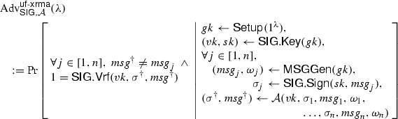
[Unforgeability against extended random message attacks ($\text {UF}\text {-}\text {XRMA}$)] A signature scheme is unforgeable against extended random message attacks (UF-XRMA) with respect to message sampler $\mathsf {MSGGen}$ if for any probabilistic polynomial-time algorithms $\mathcal{A}$ and any positive integer n bounded by a polynomial in $\lambda$, the following advantage function $\text {Adv} ^{\mathsf {uf}\text {-}\mathsf {xrma}}_{\mathsf {SIG},\mathcal{A}}$ is bounded by a negligible function in $\lambda$.

For the above security notions,$\text {UF}\text {-}\text {CMA}\Rightarrow \text {UF}\text {-}\text {XRMA}\Rightarrow \text {UF}\text {-}\text {RMA}$ holds. More precisely, for any signature scheme $\mathsf {SIG}$, for any $\mathcal{A}'$ there exists $\mathcal{A}$ such that $\text {Adv} ^{\mathsf {uf}\text {-}\mathsf cma }_{\mathsf {SIG},\mathcal{A}}(\lambda ) \!\ge \! \text {Adv} ^{\mathsf {uf}\text {-}\mathsf {xrma}}_{\mathsf {SIG},\mathcal{A}'}(\lambda )$, and for any $\mathcal{A}''$ there exists $\mathcal{A}'$ such that $\text {Adv} ^{\mathsf {uf}\text {-}\mathsf {xrma}}_{\mathsf {SIG},\mathcal{A}'}(\lambda ) \!\ge \! \text {Adv} ^{\mathsf {uf}\text {-}\mathsf {rma}}_{\mathsf {SIG},\mathcal{A}''}(\lambda )$.

3.3 Partial One-Time and Tagged One-Time Signatures

Partial one-time signatures, also known as two-tier signatures [12], are a variation of one-time signatures where only part of the public-key and secret-key must be updated for every signing, while the remaining part can be persistent.

Definition 12

(Partial one-time signature scheme [12]) A partial one-time signature scheme $\mathsf {POS}$ is a set of polynomial-time algorithms $\mathsf {POS}.\{\mathsf {Key},\mathsf {Update}, \mathsf {Sign}, \mathsf {Vrf}\}$.

• $\mathsf {POS}.\mathsf {Key} (gk)$ generates a long-term public-key $pk$ and secret-key $sk$, and sets the associated message space to be $\mathcal{M}_{o}$ as defined by $gk$ (Recall that we require that $\mathcal{M}_{o}$ be completely defined by $gk$).

• $\mathsf {POS}.\mathsf {Update} (gk)$ takes $gk$ as input, and outputs a one-time key pair $( opk , osk )$. We denote the space for $opk$ by $\mathcal{K}_{ opk }$.

• $\mathsf {POS}.\mathsf {Sign} ( sk , msg , osk )$ outputs a signature $\sigma$ on message $msg$ based on $sk$ and $osk$.

• $\mathsf {POS}.\mathsf {Vrf} ( pk , opk , msg , \sigma )$ outputs 1 for acceptance, or 0 for rejection.

Correctness requires that $1 = \mathsf {POS}.\mathsf {Vrf} ( pk , opk , msg , \sigma )$ holds except for negligible probability for any $gk,\, pk ,\, opk ,\,\sigma$, and $msg \in \mathcal{M}_{o}$, such that $gk \leftarrow \mathsf {Setup}(1^{\lambda }),\,( pk , sk ) \leftarrow \mathsf {POS}.\mathsf {Key} (gk),\,( opk , osk ) \leftarrow \mathsf {POS}.\mathsf {Update} (gk),\,\sigma \leftarrow \mathsf {POS}.\mathsf {Sign} ( sk , msg , osk )$.

A tagged one-time signature scheme is a signature scheme whose signing function in addition to the long-term secret-key takes a tag as input. A tag is one-time, i.e., it must be different for every signing.

Definition 13

(Tagged one-time signature scheme) A tagged one-time signature scheme $\mathsf {TOS}$ is a set of polynomial-time algorithms $\mathsf {TOS}.\{\mathsf {Key},\mathsf {Tag}, \mathsf {Sign}, \mathsf {Vrf}\}$.

• $\mathsf {TOS}.\mathsf {Key} (gk)$ generates a long-term public-key $pk$ and secret-key $sk$, and sets the associated message space to be $\mathcal{M}_{t}$ as defined by $gk$.

• $\mathsf {TOS}.\mathsf {Tag} (gk)$ takes $gk$ as input and outputs $tag$. By $\mathcal{T}$, we denote the space for $tag$.

• $\mathsf {TOS}.\mathsf {Sign} ( sk , msg , tag )$ outputs signature $\sigma$ for message $msg$ based on $sk$ and $tag$.

• $\mathsf {TOS}.\mathsf {Vrf} ( pk , tag , msg , \sigma )$ outputs 1 for acceptance, or 0 for rejection.

Correctness requires that $1 = \mathsf {TOS}.\mathsf {Vrf} ( pk , tag , msg , \sigma )$ holds except for negligible probability for any $gk,\, pk ,\, tag ,\,\sigma$, and $msg \in \mathcal{M}_{t}$, such that $gk \leftarrow \mathsf {Setup}(1^{\lambda }),\,( pk , sk ) \leftarrow \mathsf {TOS}.\mathsf {Key} (gk),\, tag \leftarrow \mathsf {TOS}.\mathsf {Tag} (gk),\,\sigma \leftarrow \mathsf {TOS}.\mathsf {Sign} ( sk , msg , tag )$.

A $\mathsf {TOS}$ scheme is a $\mathsf {POS}$ scheme for which $tag = osk = opk$. We can thus give a security notion for $\mathsf {POS}$ schemes that also applies to $\mathsf {TOS}$ schemes by reading $\mathsf {Update}= \mathsf {Tag}$ and $tag = osk = opk$.

Definition 14

(Unforgeability against one-time adaptive chosen message attacks) A partial one-time signature scheme is unforgeable against one-time adaptive chosen message attacks (OT-CMA) if for any probabilistic polynomial-time oracle algorithms $\mathcal{A}$ the following advantage function $\text {Adv} ^{\mathsf {ot}\text {-}\mathsf {cma}}_{\mathsf {POS},\mathcal{A}}$ is negligible in $\lambda$.

$$\begin{aligned}&\text {Adv} ^{\mathsf {ot}\text {-}\mathsf {cma}}_{\mathsf {POS},\mathcal{A}}(\lambda ) \\&\quad :=\Pr \left[ \begin{array}{l} \exists ( opk , msg ,\sigma ) \in Q_m\, \text {s.t.}\\ opk ^{\dagger } = opk \; \wedge \; msg ^{\dagger } \ne msg \; \wedge \;\\ 1 = \mathsf {POS}.\mathsf {Vrf} ( pk , opk ^{\dagger },\sigma ^{\dagger }, msg ^{\dagger }) \end{array} \,\left| \, \begin{array}{l} gk\leftarrow \mathsf {Setup}(1^\lambda ),\\ ( pk , sk ) \leftarrow \mathsf {POS}.\mathsf {Key} (gk),\\ ( opk ^{\dagger }, \sigma ^{\dagger }, msg ^{\dagger }) \leftarrow \mathcal{A}^{\mathcal{O}_t,\mathcal{O}_s}( pk )\\ \end{array} \right. \right] \end{aligned}$$

$Q_m$ is initially an empty list. $\mathcal{O}_t$ is the one-time key generation oracle that on receiving a request invokes a fresh session j, performs $( opk _j, osk _j)\leftarrow \mathsf {POS}.\mathsf {Update} (gk)$, and returns $opk _j$. $\mathcal{O}_s$ is the signing oracle that, on receiving a message $msg _j$ for session j, performs $\sigma _j \!\!\leftarrow \! \mathsf {POS}.\mathsf {Sign} ( sk , msg _j, osk _j)$, returns $\sigma _j$ to $\mathcal{A}$, and records $( opk _j, msg _j, \sigma _j)$ to the list $Q_m$. $\mathcal{O}_s$ works only once for each session. Strong unforgeability is defined by replacing condition $msg ^{\dagger } \ne msg$ with $( msg ^{\dagger }, \sigma ^{\dagger }) \ne ( msg , \sigma )$.

We define a non-adaptive variant (OT-NACMA) of the above notion by integrating $\mathcal{O}_t$ into $\mathcal{O}_s$ so that $opk _j$ and $\sigma _j$ are returned to $\mathcal{A}$ at the same time. Namely, $\mathcal{A}$ must submit $msg _j$ before seeing $opk _j$. If a scheme is secure in the sense of $\text {OT}\text {-}\text {CMA}$, the scheme is also secure in the sense of $\text {OT}\text {-}\text {NACMA}$. By $\text {Adv} ^{\mathsf {ot}\text {-}\mathsf {nacma}}_{\mathsf {POS},\mathcal{A}}(\lambda )$ we denote the advantage of $\mathcal{A}$ in this non-adaptive case. For $\mathsf {TOS}$, we use the same notation, OT-CMA and OT-NACMA, and define advantage functions $\text {Adv} ^{\mathsf {ot}\text {-}\mathsf {cma}}_{\mathsf {TOS},\mathcal{A}}$ and $\text {Adv} ^{\mathsf {ot}\text {-}\mathsf {nacma}}_{\mathsf {TOS},\mathcal{A}}$ accordingly. We will also consider strong unforgeability, for which we use labels $\mathsf {sot}\text {-}\mathsf {cma}$ and $\mathsf {sot}\text {-}\mathsf {nacma}$. Recall that if a scheme is strongly unforgeable, it is unforgeable as well.

We define a condition that is relevant for coupling random message secure signature schemes with partial one-time and tagged one-time signature schemes in later sections.

Definition 15

(Tag/one-time public-key uniformity) A $\mathsf {TOS}$ is called uniform tag if $\mathsf {TOS}.\mathsf {Tag}$ outputs $tag$ that is uniformly distributed over tag space $\mathcal{T}$. Similarly, a $\mathsf {POS}$ is called uniform-key if $\mathsf {POS}.\mathsf {Update}$ outputs $opk$ that is uniformly distributed over key space $\mathcal{K}_{ opk }$.

3.4 Structure-Preserving Signatures

A signature scheme is structure-preserving over a bilinear group $\varLambda$, if public-keys, signatures, and messages are all source group elements of $\varLambda$, and the verification only evaluates pairing product equations. Similarly, $\mathsf {POS}$ and $\mathsf {TOS}$ schemes are structure-preserving if their public-keys, signatures, messages, and tags or one-time public-keys consist of source group elements and the verification only evaluates pairing product equations.

4 Generic Constructions

4.1 $\mathsf {SIG{1}}$: Combining Tagged One-Time and RMA-Secure Signatures

Let $\mathsf {{r}SIG{}}$ be a signature scheme with message space $\mathcal{M}_{\mathsf {{r}}}$, and ${{\mathsf {TOS}}{}}$ be a tagged one-time signature scheme with tag space $\mathcal{T}$ such that $\mathcal{M}_{\mathsf {{r}}} = \mathcal{T}$ and both schemes use the same $\mathsf {Setup}$. We construct a signature scheme $\mathsf {SIG{1}}$ from $\mathsf {{r}SIG{}}$ and ${{\mathsf {TOS}}{}}$. Let $gk$ be the global parameter generated by $\mathsf {Setup}(1^\lambda )$. It is assumed that a secret-key of $\mathsf {{r}SIG{}}$ includes $gk$.

[Generic Construction 1: $\mathsf {SIG{1}}$ ]

• $\mathsf {SIG{1}}.\mathsf {Key} (gk)$: Run $( pk _{t}, sk _{t}) \leftarrow \mathsf {TOS}.\mathsf {Key} (gk),\,(vk _{r},sk _{r}) \leftarrow \mathsf {{r}SIG{}}.\mathsf {Key} (gk)$. Output $vk :=( pk _{t},vk _{r})$ and $sk :=( sk _{t},sk _{r})$.

• $\mathsf {SIG{1}}.\mathsf {Sign} (sk, msg )$: Parse $sk$ into $( sk _{t},sk _{r})$ and take $gk$ from $sk _{r}$. Run $tag \leftarrow \mathsf {TOS}.\mathsf {Tag} (gk),\,\sigma _{t} \leftarrow \mathsf {TOS}.\mathsf {Sign} ( sk _{t}, msg , tag ),\,\sigma _{r} \leftarrow \mathsf {{r}SIG{}}.\mathsf {Sign} (sk _{r}, tag )$. Output $\sigma :=( tag , \sigma _{t}, \sigma _{r})$.

• $\mathsf {SIG{1}}.\mathsf {Vrf} (vk, msg , \sigma )$: Parse $vk$ and $\sigma$ accordingly. Output 1 if $1 = \mathsf {TOS}.\mathsf {Vrf} ( pk _{t}, tag , msg , \sigma _{t})$ and $1 = \mathsf {{r}SIG{}}.\mathsf {Vrf} (vk _{r}, tag , \sigma _{r})$. Output 0 otherwise.

We prove that $\mathsf {SIG{1}}$ is secure by showing a reduction to the security of each component. As our reductions are efficient in their running time, we only relate success probabilities.

Theorem 1

$\mathsf {SIG{1}}$ is UF-CMA if $\mathsf {TOS}$ is uniform tag and OT-NACMA, and $\mathsf {{r}SIG{}}$ is UF-RMA. In particular, for any p.p.t. algorithm $\mathcal{A}$ there exist p.p.t. algorithms $\mathcal{B}$ and $\mathcal{C}$ such that $\text {Adv} ^{\mathsf {uf}\text {-}\mathsf cma }_{\mathsf {SIG{1}},\mathcal{A}}(\lambda ) \le \text {Adv} ^{\mathsf {ot}\text {-}\mathsf {nacma}}_{\mathsf {TOS},\mathcal{B}}(\lambda ) + \text {Adv} ^{\mathsf {uf}\text {-}\mathsf {rma}}_{\mathsf {{r}SIG{}},\mathcal{C}}(\lambda )$.

Security against random message attacks is sufficient for $\mathsf {{r}SIG{}}$ as it is used only to sign uniformly chosen tags. To formally prove it, however, we use the important fact that the signing function of $\mathsf {TOS}$ does not require any secret behind the tags. Departing from the $\text {UF}\text {-}\text {CMA}$ game for $\mathsf {SIG{1}}$, the security proof is done by evaluating two game transitions. The first transition is based on the $\text {OT}\text {-}\text {NACMA}$ security of $\mathsf {TOS}$. This part is rather simple as we can construct a simulator in a straightforward manner by following the key generation and signing of $\mathsf {{r}SIG{}}$. The second transition is based on $\text {UF}\text {-}\text {RMA}$ of $\mathsf {{r}SIG{}}$. We construct a simulator that, given signatures of $\mathsf {{r}SIG{}}$ on uniformly chosen tags as messages, simulates signatures of $\mathsf {SIG{1}}$ for messages provided by the adversary. For this to be done, the simulator needs to compute one-time signatures of $\mathsf {TOS}$ for the given uniform tags. This, however, can be done without any problem since the simulator has legitimate signing keys that are sufficient to run the signing function of $\mathsf {TOS}$ with uniform tags.

Proof

Any signature that is accepted as a successful forgery must either reuse an existing tag, or sign a new tag. We show that the former case reduces to attacking $\mathsf {TOS}$ and the latter case reduces to attacking $\mathsf {{r}SIG{}}$. Thus the success probability $\text {Adv} ^{\mathsf {uf}\text {-}\mathsf cma }_{\mathsf {SIG{1}},\mathcal{A}}(\lambda )$ of an attacker on $\mathsf {SIG{1}}$ will be bounded by the sum of the success probabilities $\text {Adv} ^{\mathsf {ot}\text {-}\mathsf {nacma}}_{\mathsf {TOS},\mathcal{B}}(\lambda )$ of an attacker on $\mathsf {TOS}$ and the success probability $\text {Adv} ^{\mathsf {uf}\text {-}\mathsf {rma}}_{\mathsf {{r}SIG{}},\mathcal{C}}(\lambda )$ of an attacker on $\mathsf {{r}SIG{}}$.

Game 0: :

The actual unforgeability game. $\Pr [\mathbf{Game 0}] = \text {Adv} ^{\mathsf {uf}\text {-}\mathsf cma }_{\mathsf {SIG{1}},\mathcal{A}}(\lambda )$.

Game 1: :

The real security game except that the winning condition is changed to no longer accept repetition of tags.

Lemma 1

$|\Pr [\mathbf{Game \,0}]- \Pr [\mathbf{Game\, 1}]| \le \text {Adv} ^{\mathsf {ot}\text {-}\mathsf {nacma}}_{\mathsf {TOS},\mathcal{B}}(\lambda )$

Proof

Attacker $\mathcal{A}$ wins in Game 0, but loses in Game 1, iff it produces a forgery that reuses a tag from a signing query. We describe a reduction $\mathcal{B}$ that uses such an attacker to break the OT-NACMA-security of $\mathsf {TOS}$. The reduction $\mathcal{B}$ receives $gk$ and $pk _{t}$ from the challenger of $\mathsf {TOS}$, sets up $vk _{r}$ and $sk _{r}$ honestly by running $\mathsf {{r}SIG{}}.\mathsf {Key} (gk)$, and provides $gk$ and $vk = (vk _{r}, pk _{t})$ to $\mathcal{A}$.

To answer a signing query, $\mathcal{B}$ uses the signing oracle of $\mathsf {TOS}$ to get $tag$ and $\sigma _{t}$, signs $tag$ using $sk _{r}$ to produce $\sigma _{r}$, and returns $( tag , \sigma _{t}, \sigma _{r})$. When $\mathcal{A}$ produces a forgery $( tag ^{\dagger }, \sigma _{t}^{\dagger }, \sigma _{r}^{\dagger })$ on message $msg ^{\dagger },\,\mathcal{B}$ outputs $( msg ^{\dagger }, tag ^{\dagger }, \sigma _{t}^{\dagger })$ as a forgery for $\mathsf {TOS}$.

Game 2: :

The fully idealized game. The winning condition is changed to reject all signatures.

Lemma 2

$|\Pr [\mathbf{Game \,1}] - Pr[\mathbf{Game \,2}]| \le \text {Adv} ^{\mathsf {uf}\text {-}\mathsf {rma}}_{\mathsf {{r}SIG{}},\mathcal{C}}(\lambda )$

Proof

Attacker $\mathcal{A}$ wins in Game 1, iff it produces a forgery with a fresh tag. We describe a reduction algorithm $\mathcal{C}$ that uses $\mathcal{A}$ to break the $\text {UF}\text {-}\text {RMA}$ security of $\mathsf {{r}SIG{}}$. Algorithm $\mathcal{C}$ receives $gk$ and $vk _{r}$, runs $( pk _{t}, sk _{t}) \leftarrow \mathsf {TOS}.\mathsf {Key} (gk)$, and provides $gk$ and $vk = (vk _{r}, pk _{t})$ to $\mathcal{A}$.

To answer signing query on message $msg$, algorithm $\mathcal{C}$ consults $\mathcal{O}_s$ and receives random message $msg _{r}\leftarrow \mathcal{T}$ and signature $\sigma _{r}$. Algorithm $\mathcal{C}$ then uses $msg _{r}$ as a tag, i.e., $tag = msg _{r}$, and creates signature $\sigma _{t}$ on $msg$ by running $\mathsf {TOS}.\mathsf {Sign} ( sk _{t}, msg , tag )$. It then returns $( tag , \sigma _{t}, \sigma _{r})$. Note that for a uniform tag $\mathsf {TOS}$ scheme $\mathsf {TOS}.\mathsf {Tag} (gk)$ would generate tags distributed uniformly over the tag space $\mathcal{T}$. Thus the reduction simulation is perfect. When $\mathcal{A}$ produces a forgery $( tag ^{\dagger }, \sigma _{t}^{\dagger }, \sigma _{r}^{\dagger })$ on $msg ^{\dagger }$, algorithm $\mathcal{C}$ outputs $( tag ^{\dagger }, \sigma _{r}^{\dagger })$ as a forgery.

Thus $\text {Adv} ^{\mathsf {uf}\text {-}\mathsf cma }_{\mathsf {SIG{1}},\mathcal{A}}(\lambda ) = \Pr [\mathbf{Game \,0}] \le \text {Adv} ^{\mathsf {ot}\text {-}\mathsf {nacma}}_{\mathsf {TOS},\mathcal{B}}(\lambda ) + \text {Adv} ^{\mathsf {uf}\text {-}\mathsf {rma}}_{\mathsf {{r}SIG{}},\mathcal{C}}(\lambda )$ as claimed.

The following theorem is immediately obtained from the construction.

Theorem 2

If $\mathsf {TOS}.\mathsf {Tag}$ produces constant-size tags and signatures in the size of input messages, the resulting $\mathsf {SIG{1}}$ produces constant-size signatures as well. Furthermore, if $\mathsf {TOS}$ and $\mathsf {{r}SIG{}}$ are structure-preserving, so is $\mathsf {SIG{1}}$.

4.2 $\mathsf {SIG{2}}$: Combining Partial One-Time and XRMA-Secure Signatures

Let $\mathsf {{x}SIG{}}$ be a signature scheme with message space $\mathcal{M}_{\mathsf {{x}}}$, and $\mathsf {POS}$ be a partial one-time signature scheme with one-time public-key space $\mathcal{K}_{ opk }$ such that $\mathcal{M}_{\mathsf {{x}}} = \mathcal{K}_{ opk }$ and both schemes use the same $\mathsf {Setup}$. We construct a signature scheme $\mathsf {SIG{2}}$ from $\mathsf {{x}SIG{}}$ and $\mathsf {POS}$. Let $gk$ be a global parameter generated by $\mathsf {Setup}(1^\lambda )$. It is assumed that a secret-key for $\mathsf {{x}SIG{}}$ contains $gk$.

[Generic Construction 2: $\mathsf {SIG{2}}$ ]

• $\mathsf {SIG{2}}.\mathsf {Key} (gk)$: Run $( pk _{p}, sk _{p}) \leftarrow \mathsf {POS}.\mathsf {Key} (gk),\,(vk _{x},sk _{x}) \leftarrow \mathsf {{x}SIG{}}.\mathsf {Key} (gk)$. Output $vk :=( pk _{p},vk _{x})$ and $sk :=( sk _{p},sk _{x})$.

• $\mathsf {SIG{2}}.\mathsf {Sign} (sk, msg )$: Parse $sk$ into $( sk _{p},sk _{x})$ and take $gk$ from $sk _{x}$. Run $( opk , osk ) \leftarrow \mathsf {POS}.\mathsf {Update} (gk),\,\sigma _{p} \leftarrow \mathsf {POS}.\mathsf {Sign} ( sk _{p}, msg , osk ),\,\sigma _{x} \leftarrow \mathsf {{x}SIG{}}.\mathsf {Sign} (sk _{x}, opk )$. Output $\sigma :=( opk , \sigma _{p}, \sigma _{x})$.

• $\mathsf {SIG{2}}.\mathsf {Vrf} (vk, msg , \sigma )$: Parse $vk$ and $\sigma$ accordingly. Output 1 if $1 = \mathsf {POS}.\mathsf {Vrf} ( pk _{p}, opk , msg , \sigma _{p})$, and $1 = \mathsf {{x}SIG{}}.\mathsf {Vrf} (vk _{x}, opk ,\sigma _{x})$. Output 0 otherwise.

Theorem 3

$\mathsf {SIG{2}}$ is UF-CMA if $\mathsf {POS}$ is uniform-key and OT-NACMA, and $\mathsf {{x}SIG{}}$ is $\text {UF}\text {-}\text {XRMA}$ relative to $\mathsf {POS}.\mathsf {Update}$ as a message generator. In particular, for any p.p.t. algorithm $\mathcal{A}$, there exist p.p.t. algorithms $\mathcal{B}$ and $\mathcal{C}$ such that $\text {Adv} ^{\mathsf {uf}\text {-}\mathsf cma }_{\mathsf {SIG{2}},\mathcal{A}}(\lambda ) \le \text {Adv} ^{\mathsf {ot}\text {-}\mathsf {nacma}}_{\mathsf {POS},\mathcal{B}}(\lambda ) + \text {Adv} ^{\mathsf {uf}\text {-}\mathsf {xrma}}_{\mathsf {{x}SIG{}},\mathcal{C}}(\lambda )$.

Proof

The proof is almost the same as that for Theorem 1. The only difference appears in constructing $\mathcal{C}$ in the second step. Since $\mathsf {POS}.\mathsf {Update}$ is used as the extended random message generator, the pair $( msg ,\omega )$ is in fact $( opk , osk )$. Given $( opk , osk )$, adversary $\mathcal{C}$ can run $\mathsf {POS}.\mathsf {Sign} ( sk , msg , osk )$ to yield legitimate signatures.

As for our first generic construction, the following theorem holds from the construction.

Theorem 4

If $\mathsf {POS}$ produces constant-size one-time public-keys and signatures in the size of input messages, the resulting $\mathsf {SIG{2}}$ produces constant-size signatures as well. Furthermore, if $\mathsf {POS}$ and $\mathsf {{x}SIG{}}$ are structure-preserving, so is $\mathsf {SIG{2}}$.

5 Instantiating $\mathsf {SIG{1}}$

We instantiate the building blocks $\mathsf {TOS}$ and $\mathsf {{r}SIG{}}$ of our first generic construction to obtain our first SPS scheme. We do so in the Type-I bilinear group setting. The resulting $\mathsf {SIG{1}}$ scheme is an efficient structure-preserving signature scheme based only on the $\text {DLIN}$ assumption.

5.1 Setup for Type-I Groups

The following setup procedure is common for all instantiations in this section. The global parameter $gk$ is given to all functions implicitly.

• $\mathsf {Setup}(1^\lambda )$: Run $\varLambda =(p,{{\mathbb G}},{{\mathbb G}}_T,e) \leftarrow {\mathcal {G}}(1^\lambda )$ and pick random generators $(G, C, F, U) \leftarrow ({{\mathbb G}}^*)^4$. Output $gk:=(\varLambda , G, C, F,U)$.

The parameter $gk$ fixes the message space $\mathcal{M}_{\mathsf {{r}}} :=\{(C^m,F^m,U^m) \in {{\mathbb G}}^3 \;|\; m \in \mathbb {Z}_p\}$ for the RMA-secure signature scheme presented in Sect. 5.3. For our generic framework to work, the tagged one-time signature schemes should have the same tag space.

5.2 Tagged One-Time Signature Scheme

Our scheme generates tags consisting of only one group element, $C^t$, which is optimally efficient in its size. However, as mentioned above, we need to adjust the tag space to match the message space of $\mathsf {{r}SIG{}}$. We thus describe the scheme with a tag in the extended form of $(C^t, F^t, U^t)$. The extended elements $F^t$ and $U^t$ can be dropped when unnecessary.

Our concrete construction of $\mathsf {TOS}$ can be seen as an adaptation of a one-time signature scheme in [7] so that it enjoys optimally short one-time public-key (i.e., a tag) with no corresponding one-time secret-key. We note that, given a $\mathsf {TOS}$, one can construct a one-time signature scheme. But the reverse is not known in general.

[Scheme ${{\mathsf {TOS}}{}}$ ]

• ${{\mathsf {TOS}}{}}.\mathsf {Key} ( gk )$: Parse $gk = (\varLambda , G, C,F,U)$. Choose $w_z,\,w_r, \mu _z,\, \mu _s, \tau$ uniformly from $\mathbb {Z}_p^*$ and compute $G_z :=G^{w_z},\,G_r :=G^{w_r},\,H_z :=G^{\mu _z},\,H_s :=G^{\mu _s},\,G_t :=G^{\tau }$ and For $i=1,\ldots ,k$, uniformly choose $\chi _i,\,\gamma _i,\,\delta _i$ from $\mathbb {Z}_p$ and compute

  $$\begin{aligned} G_i :=G_z^{\chi _i} G_r^{\gamma _i}, \quad \text {and} \quad H_i :=H_z^{\chi _i} H_s^{\delta _i}. \end{aligned}$$

  (1)

  Output $pk :=(G_z,\, G_r, H_z,\, H_s, G_t,\, G_1, \ldots ,G_k, H_1, \ldots ,H_k )\in {{\mathbb G}}^{2k+5}$ and $sk :=(w_r, \mu _s, \tau , \chi _1,\gamma _1,\delta _1, \ldots , \chi _k,\gamma _k,\delta _k, ) \in \mathbb {Z}_p^{3k+5}$.

• ${{\mathsf {TOS}}{}}.\mathsf {Tag} (gk)$: Choose $t \leftarrow \mathbb {Z}_p^*$, compute $T :=C^t$. Output $tag :=(T, T', T'') = (C^{t},F^t,U^t) \in {{\mathbb G}}^3$.

• ${{\mathsf {TOS}}{}}.\mathsf {Sign} ( sk , msg , tag )$: Parse $msg$ as $(\tilde{M}_1,\ldots ,\tilde{M}_k)$ and $tag$ as $(T,T', T'')$. Parse $sk$ accordingly. Choose $\zeta \leftarrow \mathbb {Z}_p$ and output $\sigma :=(\tilde{Z}, \tilde{R}, S) \in {{\mathbb G}}^3$ where

  $$\begin{aligned} \begin{array}{ll} \tilde{Z}:=G^{\zeta } \prod \limits _{i=1}^{k} \tilde{M}_i^{-\chi _i},\quad \tilde{R}:=\left( T^{\tau } G_z^{-\zeta }\right) ^{\frac{1}{w_r}} \prod \limits _{i=1}^{k} \tilde{M}_i^{-\gamma _i}, \text{ and } S\!:=\! \left( H_z^{-\zeta }\right) ^{\frac{1}{\mu _s}} \prod \limits _{i=1}^{k} \tilde{M}_i^{-\delta _i}. \end{array} \end{aligned}$$

• ${{\mathsf {TOS}}{}}.\mathsf {Vrf} ( pk , tag , msg ,\sigma )$: Parse $\sigma$ as $(\tilde{Z},\tilde{R}, S) \in {{\mathbb G}}^3,\, msg$ as $(\tilde{M}_1,\ldots ,\tilde{M}_k) \in {{\mathbb G}}^k$, and $tag$ as $(T,T', T'')$. Return 1 if the following equations hold. Return 0, otherwise.

  $$\begin{aligned} e(T, G_t)&= e\left( G_z, \tilde{Z}\right) \; e\left( G_r, \tilde{R}\right) \; \prod _{i=1}^{k} e(G_i, \tilde{M}_i) \end{aligned}$$

  (2)
  $$\begin{aligned} 1&= e\left( H_z, \tilde{Z}\right) \; e\left( H_s, S\right) \; \prod _{i=1}^{k} e\left( H_i, \tilde{M}_i\right) \end{aligned}$$

  (3)

Correctness is verified by inspecting the following relations.

$$\begin{aligned} \text {For (2):}\;&e\left( G_z, G^\zeta \prod _{i=1}^{k} \tilde{M}_i^{-\chi _i}\right) \; e\left( G_r, \left( T^{\tau } G_z^{-\zeta }\right) ^{\frac{1}{w_r}} \prod _{i=1}^{k} \tilde{M}_i^{-\gamma _i}\right) \; \prod _{i=1}^{k} e\left( G_z^{\chi _i} G_r^{\gamma _i}, \tilde{M}_i\right) \\&=e\left( G_z, G^\zeta \right) \; e\left( G, T^{\tau }\right) e\left( G, G_z^{-\zeta }\right) =e\left( G, T^{\tau }\right) =e\left( T, G_t\right) \\ \text {For (3):}\;&e\left( H_z, G^\zeta \prod _{i=1}^{k} \tilde{M}_i^{-\chi _i}\right) \; e\left( H_s, \left( H_z^{-\zeta }\right) ^{\frac{1}{\mu _s}} \prod _{i=1}^{k} \tilde{M}_i^{-\delta _i}\right) \; \prod _{i=1}^{k} e\left( H_z^{\chi _i} H_s^{\delta _i}, \tilde{M}_i\right) \\&=e\left( H_z, G^\zeta \right) \; e\left( G, H_z^{-\zeta }\right) =1 \end{aligned}$$

We state the following theorems, of which the first one is immediate from the construction.

Theorem 5

The above $\mathsf {TOS}$ is structure-preserving, and yields uniform tags and constant-size signatures.

Theorem 6

The above ${{\mathsf {TOS}}{}}$ is strongly unforgeable against one-time tag adaptive chosen message attacks (SOT-CMA) if the $\text {SDP}$ assumption holds. In particular, for all p.p.t. algorithms $\mathcal{A}$, there exists p.p.t. algorithm $\mathcal{B}$ such that $\text {Adv} ^{\mathsf {sot}\text {-}\mathsf {cma}}_{{{\mathsf {TOS}}{,}}\mathcal{A}}(\lambda )\le \text {Adv} ^{\mathsf {sdp}}_{{\mathcal {G}},\mathcal{B}}(\lambda ) + 1/p(\lambda )$, where $p(\lambda )$ is the size of the groups produced by ${\mathcal {G}}$. Moreover, the run-time overhead of the reduction $\mathcal{B}$ is a small number of multi-exponentiations per signing or tag query.

Proof

Given successful forger $\mathcal{A}$ against ${{\mathsf {TOS}}{}}$ as a black-box, we construct $\mathcal{B}$ that breaks $\text {SDP}$ as follows. Let $I_{\mathsf {sdp}}=(\varLambda , G_z, G_r, H_z, H_s)$ be an instance of ${\text {SDP}}$. Algorithm $\mathcal{B}$ simulates the attack game against ${{\mathsf {TOS}}{}}$ as follows. It first builds $gk:=(\varLambda , G, C,F,U)$ by choosing $G$ randomly from ${{\mathbb G}}^*$, choosing $c,f,u\leftarrow \mathbb {Z}_p$, and computing $C= G^c, F = G^f$, and $U = G^u$. This yields a $gk$ in the same distribution as produced by $\mathsf {Setup}$. Next $\mathcal{B}$ simulates ${{\mathsf {TOS}}{}}.\mathsf {Key}$ by taking $(G_z, G_r, H_z, H_s)$ from $I_{\mathsf {sdp}}$ and computing $G_t :=H_s^{\tau }$ for random $\tau$ in $\mathbb {Z}_p^*$. It then generates $G_i$ and $H_i$ according to (1). This perfectly simulates ${{\mathsf {TOS}}{}}.\mathsf {Key}$.

On receiving the jth query to $\mathcal{O}_t$, algorithm $\mathcal{B}$ computes

$$\begin{aligned} T :=\left( G_z^{\zeta } G_r^{\rho }\right) ^{\frac{1}{\tau }} \end{aligned}$$

(4)

for $\zeta , \rho \leftarrow \mathbb {Z}_p^*$. If $T=1,\,\mathcal{B}$ sets $Z^{\star } :=H_s,\,S^{\star } :=H_z^{-1}$, and $R^{\star } :=(Z^{\star })^{\rho /\zeta }$, outputs $(Z^{\star },R^{\star },S^{\star })$ and stops. Otherwise, $\mathcal{B}$ stores $(\zeta , \rho )$ and returns $tag _j :=(T, T^{f/c}, T^{u/c})$ to $\mathcal{A}$.

On receiving signing query $msg _j = (\tilde{M}_1,\ldots ,\tilde{M}_k)$, algorithm $\mathcal{B}$ takes $\zeta$ and $\rho$ used for computing $tag_j$ (if $tag_j$ is not yet defined, execute the above procedure for generating $tag_j$ and take new $\zeta$ and $\rho$) and computes

$$\begin{aligned}&\tilde{Z}:=H_s^{\zeta } \prod _{i=1}^{k} \tilde{M}_i^{-\chi _i},&\tilde{R}:=H_s^{\rho } \prod _{i=1}^{k} \tilde{M}_i^{-\gamma _i}, \quad \text {and}&S:=H_z^{- \zeta } \prod _{i=1}^{k} \tilde{M}_i^{-\delta _i}. \end{aligned}$$

(5)

Then $\mathcal{B}$ returns $\sigma _j :=(Z,R,S)$ to $\mathcal{A}$ and records $( tag _j, \sigma _j, msg _j)$.

When $\mathcal{A}$ outputs a forgery $( tag ^{\dagger },\sigma ^{\dagger }, msg ^{\dagger })$, algorithm $\mathcal{B}$ searches the records for $( tag , \sigma , msg )$ such that $tag ^{\dagger } = tag$ and $( msg ^{\dagger },\sigma ^{\dagger }) \ne ( msg , \sigma )$. If no such entry exists, $\mathcal{B}$ aborts. Otherwise, $\mathcal{B}$ computes

$$\begin{aligned} \tilde{Z}^{\star } :=\frac{\tilde{Z}^{\dagger }}{\tilde{Z}} \prod _{i=1}^{k} \left( \frac{\tilde{M}^{\dagger }_i}{\tilde{M}_i}\right) ^{\chi _i},\quad \tilde{R}^{\star } :=\frac{\tilde{R}^{\dagger }}{\tilde{R}} \prod _{i=1}^{k} \left( \frac{\tilde{M}^{\dagger }_i}{\tilde{M}_i}\right) ^{\gamma _i}, \;\text {and}\quad S^{\star } :=\frac{S^{\dagger }}{S} \prod _{i=1}^{k} \left( \frac{\tilde{M}^{\dagger }_i}{\tilde{M}_i}\right) ^{\delta _i} \end{aligned}$$

where $(\tilde{Z},\tilde{R},S),\,(\tilde{M}_1,\ldots ,\tilde{M}_k)$ and their dagger counterparts are taken from $(\sigma , msg )$ and $(\sigma ^{\dagger }, msg ^{\dagger })$, respectively. $\mathcal{B}$ finally outputs $(\tilde{Z}^{\star },\tilde{R}^{\star }, S^{\star })$ and stops. This completes the description of $\mathcal{B}$.

We claim that $\mathcal{B}$ solves the problem by itself or the view of $\mathcal{A}$ is perfectly simulated. The correctness of key generation has been already inspected. In the simulation of $\mathcal{O}_t$, there is a case of $T=1$ that happens with probability 1 / p. If it happens, $\mathcal{B}$ outputs a correct answer to $I_{\mathsf {sdp}}$, which is clear by observing $G_z=G_r^{-\rho /\zeta },\,Z^{\star } = H_s \ne 1,\,e(G_z, Z^{\star })e(G_r, R^{\star }) = e(G_r^{-\rho /\zeta }, Z^{\star })e(G_r, (Z^{\star })^{\rho /\zeta })=1$ and $e(H_z, Z^{\star }) e(H_s, S^{\star }) = e(H_z, H_s) e(H_s, H_z^{-1}) = 1$. Otherwise, tag T is uniformly distributed over ${{\mathbb G}}^*$ and the simulation is perfect.

Oracle $\mathcal{O}_s$ is simulated perfectly as well. Correctness of simulated $\sigma _j = (\tilde{Z},\, \tilde{R},\, S)$ can be verified by inspecting the following relations.

$$\begin{aligned} \text {(Right-hand of (2))}&= e\left( G_z, H_s^{\zeta } \prod _{i=1}^{k} \tilde{M}_i^{-\chi _i}\right) \; e\left( G_r, H_s^{\rho } \prod _{i=1}^{k} \tilde{M}_i^{-\gamma _i}\right) \\&\quad \times \prod _{i=1}^{k} e\left( G_z^{\chi _i} G_r^{\gamma _i}, \tilde{M}_i\right) \\&=e\left( G_z^{\zeta } G_r^{\rho }, H_s\right) =e\left( \left( G_z^{\zeta } G_r^{\rho }\right) ^{\frac{1}{\tau }}, H_s^{\tau }\right) =e(T_1, G_t) \\ \text {(Right-hand of (3))}&= e\left( H_z, H_s^{\zeta } \prod _{i=1}^{k} \tilde{M}_i^{-\chi _i}\right) e\left( H_s, H_z^{- \zeta } \prod _{i=1}^{k} \tilde{M}_i^{-\delta _i}\right) \prod _{i=1}^{k} e(H_z^{\chi _i} H_s^{\delta _i}, \tilde{M}_i)\\&=e\left( H_z, H_s^{\zeta }\right) \; e\left( H_s, H_z^{- \zeta }\right) \; = 1 \end{aligned}$$

Every $\tilde{Z}$ is uniformly distributed over ${{\mathbb G}}$ due to the uniform choice of $\zeta$. Then $\tilde{R}$ and $S$ are uniquely determined by following the distribution of $\tilde{Z}$.

Accordingly, $\mathcal{A}$ outputs a successful forgery with non-negligible probability and $\mathcal{B}$ finds a corresponding record $( tag ,\sigma , msg )$. We show that output $(\tilde{Z}^{\star }, \tilde{R}^{\star }, S^{\star })$ from $\mathcal{B}$ is a valid solution to $I_{\mathsf {sdp}}$. First, Eq. (2) is satisfied because

$$\begin{aligned} 1&= e\left( G_z, \frac{\tilde{Z}^{\dagger }}{\tilde{Z}}\right) \; e\left( G_r, \frac{\tilde{R}^{\dagger }}{\tilde{R}}\right) \prod _{i=1}^{k} e\left( G_z^{\chi _i} G_r^{\gamma _i}, \frac{\tilde{M}^{\dagger }_i}{\tilde{M}_i}\right) \\&= e\left( G_z, \frac{\tilde{Z}^{\dagger }}{\tilde{Z}} \prod _{i=1}^{k} \left( \frac{\tilde{M}^{\dagger }_i}{M_i}\right) ^{\chi _i}\right) \; e\left( G_r, \frac{\tilde{R}^{\dagger }}{\tilde{R}} \prod _{i=1}^{k} \left( \frac{\tilde{M}^{\dagger }_i}{M_i}\right) ^{\gamma _i}\right) \\&= e\left( G_z, \tilde{Z}^{\star }\right) \; e\left( G_r, \tilde{R}^{\star }\right) , \end{aligned}$$

holds. Equation (3) can be verified similarly.

It remains to prove that $\tilde{Z}^{\star } \ne 1$. Note that, if $msg = msg ^{\dagger }$ but this is still a valid forgery then it must be the case that $(\tilde{Z}, \tilde{R})\ne (\tilde{Z}^{\dagger }, \tilde{R}^{\dagger })$. Since $\tilde{R}$ (resp. $\tilde{R}^{\dagger }$) is uniquely determined by $\tilde{Z}$ and $msg$ (resp. $\tilde{Z}^{\dagger }, msg ^{\dagger }$), that would mean that $\tilde{Z}^{\star }\ne 1$. Alternatively, if $msg ^{\dagger } \ne msg$, then there exists $\ell \in \{1,\ldots ,k\}$ such that $\tilde{M}^{\dagger }_{\ell }/{M_{\ell }}\ne 1$. We claim that parameters $\chi _1,\ldots ,\chi _k$ are independent of the view of $\mathcal{A}$. We prove it by showing that, for every possible assignment to $\chi _1,\ldots ,\chi _k$, there exists an assignment to other coins, i.e., $(\gamma _1,\ldots ,\gamma _k,\, \delta _1,\ldots ,\delta _k)$ and $(\zeta ^{(1)}, \rho ^{(1)},\ldots , \zeta ^{(q_s)}, \rho ^{(q_s)})$ for $q_s$ queries, that is consistent with the view of $\mathcal{A}$ (By $\zeta ^{(j)}$, we denote $\zeta$ with respect to the jth query. We follow this convention hereafter. Without loss of generality, we assume that $\mathcal{A}$ makes $q_s$ tag queries and the same number of signing queries). Observe that the view of $\mathcal{A}$ consists of independent group elements $(G, G_z, G_r, H_z, H_s, G_t, G_1, H_1,\ldots ,G_k, H_k)$ and $(T_1^{(j)}, \tilde{Z}^{(j)}, \tilde{M}^{(j)}_1, \ldots , \tilde{M}^{(j)}_k)$ for $j=1,\ldots ,q_s$ (Note that we omit $\tilde{R}^{(j)}$ and $S^{(j)}$ from the view since they are uniquely determined by the other components). We represent the view by the discrete logarithms of these group elements with respect to base $G$. Namely, the view is represented by $(1, w_z, w_r, \mu _z, \mu _s, \tau , w_1, \mu _1,\ldots , w_k, \mu _k)$ and $(t^{(j)}, z^{(j)}, m^{(j)}_1,\ldots ,m^{(j)}_k)$ for $j=1,\ldots ,q_s$. The view and the random coins follow relations from (1), (4), and (5), which translate to

$$\begin{aligned}&w_i = w_z \chi _i + w_r \gamma _i, \quad \mu _i = \mu _z \chi _i + \mu _s \delta _i \quad \text { for } i=1,\ldots ,k, \end{aligned}$$

(6)

$$\begin{aligned}&\tau t^{(j)} = w_z \zeta ^{(j)} + w_r \rho ^{(j)}, \;\text {and} \end{aligned}$$

(7)

$$\begin{aligned}&z^{(j)} = \mu _s\,\zeta ^{(j)} - \sum _{i=1}^{k} m^{(j)}_i \chi _i \quad \text { for } j=1,\ldots ,q_s. \end{aligned}$$

(8)

For any $\ell \in \{1,\ldots ,k\}$, fix $\chi _1,\ldots , \chi _{\ell -1},\chi _{\ell +1},\ldots , \chi _k$, and consider $\chi _\ell$. For every value of $\chi _\ell$ in $\mathbb {Z}_p$, the linear equations in (6) determine $\gamma _\ell$ and $\delta _\ell$. Then, if $m^{(j)}_\ell \ne 0$, equation (8) determines $\zeta ^{(j)}$, and $\rho ^{(j)}$ follows from equation (7). If $m^{(j)}_\ell = 0$, then $\zeta ^{(j)},\,\rho ^{(j)}$ can be assigned independently from $\chi _\ell$. The above holds for every $\ell$ in $\{1,\ldots ,k\}$. Thus, if $(\chi _1,\ldots ,\chi _k)$ is distributed uniformly over $\mathbb {Z}_p^k$, then other coins are distributed uniformly as well and the view of $\mathcal{A}$ is still consistent.

Now we see that given $\mathcal{A}$’s view, $\left( {M^{\dagger }_{\ell }}/{M_{\ell }}\right) ^{\chi _{\ell }}$ is distributed uniformly over ${{\mathbb G}}$ and independent of the other $\{\chi _i\}_{i\ne \ell }$. Therefore $Z^{\star } = 1$ happens only with probability 1 / p. Thus, $\mathcal{B}$ outputs a valid $(Z^{\star }, R^{\star },S^{\star })$ with probability $\text {Adv} ^{\mathsf {sdp}}_{{\mathcal {G}},\mathcal{B}} = 1/p + (1-1/p) (1-1/p) \text {Adv} ^{\mathsf {sot}\text {-}\mathsf {cma}}_{{{\mathsf {TOS}}{}},\mathcal{A}}$, which leads to $\text {Adv} ^{\mathsf {sot}\text {-}\mathsf {cma}}_{{{\mathsf {TOS}}{}},\mathcal{A}} \le \text {Adv} ^{\mathsf {sdp}}_{{\mathcal {G}},\mathcal{B}} + 1/p$ as claimed. $\square$

Remark 1

The above TOS does not trivially work in the Type-III setting since computing R from T in signing, simulating T using $G_r$ in the reduction, and computing pairing $e(G_r,R)$ in the verification cannot be consistent. In a very recent paper [AGOT14], it is claimed that it can work if some extra group elements are given in public-keys and the underlying assumption, though the resulting scheme would be slightly less efficient than our dedicated construction in the Type-III setting.

Remark 2

The $\mathsf {TOS}$ can be used to sign messages of unbounded length by chaining the signatures. Every message block except for the last one is followed by a tag used to sign the next block. The signature consists of all internal signatures and tags. The initial tag is considered as the tag for the entire signature. For a message consisting of m group elements, it repeats $\tau :=1 + \max (0,\lceil \frac{m-k}{k-1} \rceil )$ times and the resulting signature consists of $4\tau -1$ elements.

5.3 RMA-Secure Signature Scheme

To sign random group elements, we will use a construction based on the dual system signature scheme of Waters [44]. For readers unfamiliar with Waters’ scheme we recall it in “Appendix.” Our intuition for making the original scheme structure-preserving is as follows. While the original scheme is CMA-secure under the $\text {DLIN}$ assumption, the security proof makes use of a trapdoor commitment to elements in $\mathbb {Z}_p$ and consequently messages are elements in $\mathbb {Z}_p$ rather than ${{\mathbb G}}$. Our construction below resorts to RMA-security and removes this commitment to allow messages to be a sequence of random group elements satisfying a particular relation. Concretely, the message space $\mathcal{M}_{\mathsf {{x}}} :=\{(C^{m},F^{m},U^{m}) \in {{\mathbb G}}^3 \;|\; m \in \mathbb {Z}_p\}$ is defined by generators (C, F, U) in $gk$. Moreover, the tag elements of Waters’ scheme are removed in our RMA-secure scheme as they were primarily required for (adaptive) $\text {CMA}$-security.

Other minor modifications are needed for the structure-preserving property. We modify the verification algorithm. Our verification algorithm is deterministic and uses five verification equations. Two equations are for signature elements that are not related to the message part—this is a consequence of deterministic verification. Three equations are for the (extended) message part. We also slightly modify the verification key. One element in ${{\mathbb G}}_T$ is divided into two elements of ${{\mathbb G}}$ via randomization due to the requirement of SPS.

[Scheme $\mathsf {{r}SIG{}}$ ]

• $\mathsf {{r}SIG{}}.\mathsf {Key} (gk)$: Given $gk:=(\varLambda , G, C, F, U)$ as input, uniformly select $V, V_1, V_2, H$ from ${{\mathbb G}}^*$ and $a_1,a_2,b,\alpha$, and $\rho$ from $\mathbb {Z}_p^*$. Then compute and output $vk :=(B, A_1, A_2$, $B_1, B_2, R_1, R_2$, $W_1, W_2, H, X_1, X_2)$ and $sk \!:=\! (vk, K_1, K_2,V,V_1,V_2)$ where

  $$\begin{aligned}&B:=G^b,&A_1:=G^{a_1},&A_2:=G^{a_2},&B_1:=G^{b \cdot a_1},&B_2:=G^{b \cdot a_2}\\&R_1:=VV_1^{a_1},&R_2:=VV_2^{a_2},&W_1:=R_1^b,&W_2:=R_2^b,\\&X_1:=G^{\rho },&X_2:=G^{\alpha \cdot a_1 \cdot b/\rho },&K_1:=G^\alpha ,&K_2:=G^{\alpha \cdot a_1}. \end{aligned}$$

• $\mathsf {{r}SIG{}}.\mathsf {Sign} (sk, msg )$: Parse $msg$ into $(M_1, M_2, M_3)$. Pick random $r_1, r_2, z_1, z_2 \in \mathbb {Z}_p$. Let $r= r_1+r_2$. Compute and output signature $\sigma :=(S_0,S_1, \ldots S_7)$ where

  $$\begin{aligned}&S_0 :=(M_3H)^{r_1},&S_1 :=K_2V^{r},&S_2 :=K_1^{-1} V_1^{r} G^{z_1},&S_3 :=B^{-z_1},\\&S_4 :=V_2^{r} G^{z_2},&S_5 :=B^{-z_2},&S_6 :=B^{r_2},&S_7 :=G^{r_1}. \end{aligned}$$

• $\mathsf {{r}SIG{}}.\mathsf {Vrf} (vk, \sigma , msg )$: Parse $msg$ into $(M_1, M_2, M_3)$ and $\sigma$ into $(S_0,S_1, \ldots , S_7)$. Also parse $vk$ accordingly. Verify the following pairing product equations:

  $$\begin{aligned}&e(S_1,B)\, e(S_2,B_1)\, e(S_3,A_1) =e(S_6,R_1)\, e(S_7,W_1), \end{aligned}$$

  (9)
  $$\begin{aligned}&e(S_1,B)\, e(S_4,B_2)\, e(S_5, A_2) = e(S_6, R_2)\, e(S_7, W_2)\, e(X_1,X_2), \end{aligned}$$

  (10)
  $$\begin{aligned}&e(S_7, M_3 H) = e(G, S_0), \end{aligned}$$

  (11)
  $$\begin{aligned}&e(F,M_1)=e(C,M_2), \end{aligned}$$

  (12)
  $$\begin{aligned}&e(U, M_1)=e(C, M_3). \end{aligned}$$

  (13)

The scheme is structure-preserving by construction, and the correctness is easily verified as follows.

$$\begin{aligned} \text{(Left-hand } \text{ of } \text{(9)) }&= e\left( G^{\alpha a_1}V^r, G^b\right) e\left( G^{-\alpha }V_1^{r}G^{z_1},G^{b a_1}\right) e\left( G^{-b z_1},G^{a_1}\right) \\&= e\left( G,V\right) ^{br} e\left( G,V_1\right) ^{b a_1 r}\\&= e\left( G,V\right) ^{b\left( r_1 + r_2\right) } e\left( G,V_1\right) ^{ba_1 \left( r_1 + r_2\right) }\\&= e\left( G^{br_2},VV_1^{a_1}\right) e\left( G^{r_1},V^{b}V_1^{b a_1}\right) \\&=\text{(Right-hand } \text{ of } (9))\\ \text{(Left-hand } \text{ of } (10))&=e\left( G^{\alpha a_1}V^r, G^b\right) e\left( V_2^{r}G^{z_2},G^{b a_2}\right) e\left( G^{-b z_2},G^{ a_2}\right) \\&=e\left( G,G\right) ^{\alpha b a_1 } e\left( G,V\right) ^{br} e\left( G,V_2\right) ^{b a_2 r}\\&=e\left( G,V\right) ^{b \left( r_1 + r_2\right) } e\left( G,V_2\right) ^{b a_2 \left( r_1 + r_2\right) } e\left( G,G\right) ^{\alpha b a_1} \\&=e\left( G^{br_2},VV_2^{a_2}\right) e\left( G^{r_1},V^{b}V_2^{b a_2}\right) e\left( G^{\rho },G^{\alpha b a_1 /\rho }\right) \\&=\text{(Right-hand } \text{ of } \text{(10)) } \end{aligned}$$

Equations (9) and (10) hold since $r= r_1 + r_2$. The followings also hold.

$$\begin{aligned}&\text{(Left-hand } \text{ of } (11))=e(G^{r_1},U^mH) =e(G,U^mH)^{r_1}=e(G,(U^mH)^{r_1})\\&\quad =\text{(Right-hand } \text{ of } (11)),\\&\text{(Left-hand } \text{ of } (12))=e(F,C^m)=e(F,C)^m =e(C,F^m)=\text{(Right-hand } \text{ of } (12)),\\&\text{(Left-hand } \text{ of } (13))=e(U,C^m)=e(U,C)^m =e(C,U^m)=\text{(Right-hand } \text{ of } (13)). \end{aligned}$$

Theorem 7

The above $\mathsf {{r}SIG{}}$ scheme is UF-RMA under the $\text {DLIN}$ assumption. In particular, for any p.p.t. algorithm $\mathcal{A}$ against $\mathsf {{r}SIG{}}$ that makes at most $q_s(\lambda )$ signing queries, there exists p.p.t. algorithm $\mathcal{B}$ for $\text {DLIN}$ such that $\text {Adv} ^{\mathsf {uf}\text {-}\mathsf {rma}}_{\mathsf {{r}SIG{}},\mathcal{A}}(\lambda ) \le (q_s(\lambda )+2) \cdot \text {Adv} ^{\mathsf {dlin}}_{{\mathcal {G}},\mathcal{B}}(\lambda )$.

Proof

We refer to the signatures output by the signing algorithm as normal signatures. In the proof we will consider an additional type of signatures which we refer to as simulation-type signatures; these will be computationally indistinguishable but easier to simulate. For $\gamma \in \mathbb {Z}_p$, simulation-type signatures are of the form $\sigma = (S_0,S_1'=S_1 \cdot G^{-a_1 a_2 \gamma }, S_2'=S_2 \cdot G^{a_2 \gamma }, S_3, S_4' = S_4 \cdot G^{a_1 \gamma }, S_5, \ldots , S_7)$ where $(S_0,\ldots , S_7)$ is a normal signature. We give the outline of the proof using some lemmas. Proofs for the lemmas are given after the outline.

Lemma 3

Any signature that is accepted by the verification algorithm must be either a normal-type signature or a simulation-type signature.

To prove this lemma, we introduced two verification equations for signature elements that are not related to a message. We consider a sequence of games. Let $p_i$ be the probability that the adversary succeeds in Game i, and $p_{i}^\text {norm}(\lambda )$ and $p_i^\text {sim}(\lambda )$ that he succeeds with a normal-type, or simulation-type forgery, respectively. Then by Lemma 3, $p_i(\lambda )=p_{i}^\text {norm}(\lambda )+p_i^\text {sim}(\lambda )$ for all i.

Game 0: :

The actual unforgeability under random message attacks game.

Lemma 4

There exists an adversary $\mathcal{B}_1$ such that $p_0^\text {sim}(\lambda ) \le \text {Adv} ^{\mathsf {dlin}}_{{\mathcal {G}},\mathcal{B}_1}(\lambda )$.

Game i: :

The real security game except that the first i signatures that are given by the oracle are simulation-type signatures.

Lemma 5

There exists an adversary $\mathcal{B}_2$ such that $|p_{i-1}^\text {norm}(\lambda )-p_{i}^\text {norm}(\lambda )| \le \text {Adv} ^{\mathsf {dlin}}_{{\mathcal {G}},\mathcal{B}_2}(\lambda )$.

Game q: :

All signatures given by the oracle are simulation-type signatures.

Lemma 6

There exists an adversary $\mathcal{B}_3$ such that $p_q^\text {norm}(\lambda ) \le \text {Adv} ^{\mathsf {cdh}}_{{\mathcal {G}},\mathcal{B}_3}(\lambda )$.

We have shown that in Game q, $\mathcal{A}$ can output a normal-type forgery with at most negligible probability. Thus, by Lemma 5 we can conclude that the same is true in Game 0 and it holds that

$$\begin{aligned} \text {Adv} ^{\mathsf {uf}\text {-}\mathsf {rma}}_{\mathsf {{r}SIG{}},\mathcal{A}}(\lambda )&= p_0(\lambda ) = p_0^\text {sim}(\lambda ) + p_0^\text {norm}(\lambda ) \le p_0^\text {sim}(\lambda ) + \sum _{i=1}^q |p_{i-1}^\text {norm}(\lambda )-p_{i}^\text {norm}(\lambda )|\\&\quad +p_q^\text {norm}(\lambda ) \\&\le \text {Adv} ^{\mathsf {dlin}}_{{\mathcal {G}},\mathcal{B}_1}(\lambda ) + q \text {Adv} ^{\mathsf {dlin}}_{{\mathcal {G}},\mathcal{B}_2}(\lambda ) + \text {Adv} ^{\mathsf {cdh}}_{{\mathcal {G}},\mathcal{B}_3}(\lambda ) \le (q+2) \cdot \text {Adv} ^{\mathsf {dlin}}_{{\mathcal {G}},\mathcal{B}}(\lambda ). \end{aligned}$$

Proof of Lemma 3

We have to show that only normal and simulation-type signatures can fulfil these equations. We ignore verification equations (12) and (13) that establish that $msg$ is well formed. A signature has four random exponents, $r_1, r_2, z_1, z_2$. A simulation-type signature has additional exponent $\gamma$.

We interpret $S_7$ as $G^{r_1}$, and it follows from verification equation (11) that $S_0$ is $(M_3 H)^{r_1}$. We interpret $S_3$ as $G^{- b z_1},\,S_5$ as $G^{- b z_2}$, and $S_6$ as $G^{r_2 b}$. Now we have fixed all exponents of a normal signature. The remaining two verification equations tell us that

$$\begin{aligned} e\left( G^b, S_1\right) \cdot e\left( G^{b a_1}, S_2\right)&= e\left( VV_1^{a_1}, G^{r_2 b}\right) \cdot e\left( \left( VV_1^{a_1}\right) ^b, G^{r_1}\right) \cdot e\left( G^{a_1}, G^{b z_1}\right) , \\ e\left( G^b, S_1\right) \cdot e\left( G^{b a_2}, S_4\right)&= e\left( VV_2^{a_2}, G^{r_2 b}\right) \cdot e\left( \left( VV_2^{a_2}\right) ^b, G^{r_1}\right) \cdot e\left( G^{a_2}, G^{b z_2}\right) \\&\quad \cdot e\left( G, G\right) ^{\alpha a_1 b}. \end{aligned}$$

We interpret $S_1$ as $G^{\alpha \cdot a_1} V^{r} G^{-a_1 a_2 \gamma }$. Now we have two equations and two unknowns that fix $S_2$ to $G^{-\alpha } V_1^rG^{z_1} G^{a_2 \gamma }$ and $S_4$ to $V_2^{r} G^{z_2} G^{a_1 \gamma }$, respectively. If $\gamma =0$ we have a normal signature, otherwise we have a simulation-type signature.

Proof of Lemma 4

Suppose for contradiction that there is an adversary $\mathcal{A}$, which, when playing Game 0 (and thus receiving only normal signatures), produces forgeries which are formed like simulation-type signatures. Then we can construct an adversary $\mathcal{B}_1$ for DLIN as follows.

Let $I_{\mathsf {dlin}} \!=\! (\varLambda , G_1, G_2, G_3, X, Y, Z)$ be an instance of $\text {DLIN}$ where $\varLambda \!=\! (p, {{\mathbb G}}, {{\mathbb G}}_T, e)$ is a Type-I bilinear group setting and $G_1,\,G_2,\,G_3$ are randomly taken from ${{\mathbb G}}^*$ and there exist random $x,y,z \in \mathbb {Z}_p$ such that $X= G_1^x,\,Y=G_2^y$ and $Z= G_3^z$ or $G_3^{x+y}$. Given $I_{\mathsf {dlin}}$, adversary $\mathcal{B}_1$ works as follows. It first sets $G:=G_3$ and chooses C, F, U at random from ${{\mathbb G}}^*$, and then sets them into gk. Next, it chooses $v, v_1, v_2 \in \mathbb {Z}_p^*$ and computes $V:=G_3^{v},\,V_1:=G_3^{v_1}$, and $V_2:=G_3^{v_2}$ (This way we know the discrete log of these values w.r.t. $G_3$). Then it chooses random $H \in {{\mathbb G}}^*,\,b, \alpha , \rho \in \mathbb {Z}_p^*$ and compute:

$$\begin{aligned} \begin{array}{llll} B:=G_3^b, &{}&{}&{}\\ A_1:=G_1, &{}\quad A_2:=G_2, &{}\quad B_1:=G_1^b, &{}\quad B_2:=G_2^b\\ R_1:=VV_1^{a_1} \,{=}\, G_3^{v} G_1^{v_1},&{}\quad R_2:=VV_2^{a_2} \,{=}\,G_3^{v} G_2^{v_2},&{}\quad W_1:=R_1^b \,{=}\, (G_3^{v} G_1^{v_1})^b,&{}\quad W_2:=R_2^b \,{=}\, (G_3^{v} G_2^{v_2})^b,\\ X_1:=G_3^{\rho }, &{}\quad X_2:=G^{\alpha \cdot a_1 \cdot b / \rho } \,{=}\, G_1^{\alpha b / \rho }, &{}\quad K_1:=G_3^\alpha , &{}\quad K_2:=G^{\alpha \cdot a_1} = G_1^\alpha . \end{array} \end{aligned}$$

and sets them into vk and sk, accordingly. Note that both the distribution of the public- and secret-keys are statistically close to that in the real $\text {DLIN}$ game. Moreover, to sign random messages, $\mathcal{B}_1$ can follow the real signing algorithm by using $sk$.

Suppose that $\mathcal{A}$ produces a valid forgery $\sigma ^{\dagger }$ and $msg ^{\dagger }$. Then $\mathcal{B}_1$ proceeds as follows. It parses $\sigma ^{\dagger }$ as $(S_0,\ldots , S_7)$. By Lemma 3, it is shown that if the verification equations hold, then it must hold that $S_1 = G^{\alpha a_1} V^{r} G^{-a_1a_2\gamma },\,S_2 = G^{-\alpha }V_1^{r} G^{z_1} G^{a_2 \gamma }$, and $S_4 = V_2^{r} G^{z_2} G^{a_1 \gamma }$. If this is a simulation-type signature, it holds that $\gamma \ne 0$. According to our choice of public-key, we can rewrite $S_1 = G_1^{\alpha } V^{r} G_2^{- f \gamma },\,S_2 = G_3^{-\alpha } V_1^{r} G_3^{z_1} G_2^{ \gamma }$, and $S_4 = V_2^{r} G_3^{z_2} G_1^{\gamma }$, where f is the discrete log of $G_1$ w.r.t. $G_3$. Thus, if $\mathcal{B}_1$ can extract $G_2^{-f \gamma }, G_2^{\gamma }, G_1^{\gamma }$, it can easily break the DLIN instance by testing whether $1 = e(Z, G_2^{-f \gamma }) \cdot e(G_2^\gamma , X) e(G_1^{\gamma }, Y)$. $\mathcal{B}_1$ can extract such values because the signature includes $S_3 = G_3^{-bz_1},\,S_5 = G_3^{-bz_2},\,S_6 = G_3^{br_2}$, and $S_7 = G_3^{r_1}$, and it has $b,\alpha$ and the discrete logarithms of $V, V_1, V_2$ w.r.t. $G_3$. Thus, it will be straightforward to extract the above values.

Proof of Lemma 5

Suppose for contradiction that there exists an adversary $\mathcal{A}$ such that the probabilities that $\mathcal{A}$ outputs a normal-type forgery in Game i and Game $i+1$ differ by a non-negligible amount. Then we will use $\mathcal{A}$ to construct an algorithm $\mathcal{B}_2$ that breaks the DLIN assumption.

$\mathcal{B}_2$ is given an instance of $\text {DLIN}$; $I_{\mathsf {dlin}} = (\varLambda , G_1, G_2, G_3, X, Y, Z)$. Note that determining whether a signature is of normal type or simulation type naturally corresponds to a DLIN problem: each signature contains $S_7=G^{r_1},\,S_6= (G^{b})^{r_2}$, and $S_1$ which will include $V^{r_1+r_2}$ or $V^{r_1+r_2} G^{-a_1a_2\gamma }$ depending on whether this is a normal- or simulation-type signature (Recall that we define $r=r_1+r_2$). If $\mathcal{B}_2$ sets $G= G_2,\,G^{b} = G_1$, and $V= G_3$, then it seems fairly straightforward to argue based on the DLIN assumption that it will be impossible for the adversary to distinguish normal and simulation-type signatures. However, $\mathcal{B}_2$ cannot tell whether $\mathcal{A}$’s forgery is normal type or simulation type in this simulation. Thus, there will be no way for $\mathcal{B}_2$ to take advantage of a change in $\mathcal{A}$’s success probability to solve the DLIN challenge.

The solution is to set things up so that, with high probability $\mathcal{B}_2$ can take $S_0$ from the adversary’s forgery and extract something that looks like $G_3^{r_1}$ (which will allow $\mathcal{B}_2$ to distinguish DLIN tuples and consequently detect simulation-type signatures), but at the same time it is guaranteed that for the ith message, the $G_3$ component of $S_0$ will cancel out, leaving only an $G_2^{r_1}$ component which will not allow the challenger itself to know whether a simulated signature is normal type or simulation type.

More specifically, the idea will be to choose some secret values $\xi ,\beta , \chi , \eta$ and embed them in the parameters so that for message $(C^w, F^w, U^w)$ we get $U^{w} H\!=\! G_2^{\chi w + \eta } G_3^{\xi w +\beta }$. Then $S_0 = (U^{w} H)^{r_1} = G_2^{(\chi w+\eta ) r_1}G_3^{(\xi w +\beta )r_1}$. If $\xi w + \beta \ne 0$, this gives useful information on $G_3^{r_1}$ (in particular it will allow $\mathcal{B}_2$ to test candidate values), while if $\xi w +\beta =0$, this has no $G_3$ component and thus doesn’t help at all with finding $G_3^{r_1}$. $\mathcal{B}_2$ chooses $\xi , \beta$ so that $\xi w + \beta =0$ for the w used to generate the ith message. Furthermore, it will be guaranteed that $\xi , \beta$ are information theoretically hidden even given w, so the adversary has only negligible chance of producing another message with $U^{w^*}$ such that $\xi w^*+\beta =0$ as well.

Now we show details of the algorithm for $\mathcal{B}_2$. First of all, $\mathcal{B}_2$ sets up the message space and generates the public-key in the following manner. $\mathcal{B}_2$ sets $(C, F)$, used to define message space $\mathcal{M}$, to $(G_1^\varphi ,G_3)$ by choosing random $\varphi \leftarrow \mathbb {Z}_p^*$. It chooses random $\xi ,\beta , \chi ,\eta \leftarrow \mathbb {Z}_p^*$, and computes $U:=G_2^{\chi } G_3^{\xi }$, and $H:=G_2^{\eta } G_3^\beta$. These values will be uniformly distributed, and independent of $\xi ,\beta$. $\mathcal{B}_2$ then sets

$$\begin{aligned} gk&= \left( \varLambda , G, C,F,U\right) :=\left( \varLambda , G_2, G_1^\varphi ,G_3, G_2^{\chi }G_3^{\xi }\right) \end{aligned}$$

$\mathcal{B}_2$ also sets $B:=G_1$, and chooses $V,V_1,V_2$. It must choose these values carefully so that it can compute both $W_i$ and $W_i^b$, and at the same time so that the component $V^{r}$ of a signature value $S_1$ gives $\mathcal{B}_2$ some useful information (in particular it will allow $\mathcal{B}_2$ to derive $G_3^{r}$). It does this by choosing $v_1, v_2, \delta \leftarrow \mathbb {Z}_p^*$, and computing $V:=G_3^{-a_1a_2\delta },\,V_1:=G_2^{v_1}G_3^{a_2\delta }$, and $V_2:=G_2^{v_2}G_3^{a_1\delta }$.

Next, $\mathcal{B}_2$ chooses $a_1, a_2, \alpha ,\rho \leftarrow \mathbb {Z}_p^*$ and computes

$$\begin{aligned} \begin{array}{llll} B:=G_1,&{}&{}&{}\\ A_1:=G_2^{a_1}, &{}\quad A_2:=G_2^{a_2}, &{}\quad B_1:=G_1^{a_1}, &{}\quad B_2:=G_1^{a_2}\\ R_1:=VV_1^{a_1} = G_2^{a_1v_1}, &{}\quad \! R_2:=VV_2^{a_2} =G_2^{a_2v_2}, &{}\quad \! W_1:=R_1^b = G_1^{a_1v_1}, &{}\quad W_2:=R_2^b = G_1^{a_2v_2},\\ X_1:=G_2^{\rho }, &{}\quad X_2:=G_1^{\alpha a_{1}/\rho }, &{}\quad K_1:=G_2^\alpha , &{}\quad K_2:=G_2^{\alpha a_1}, \end{array} \end{aligned}$$

and sets them into vk and sk, accordingly. Note that both of these tuples are distributed statistically close to those produced by $\mathsf {Setup}$ and $\mathsf {{r}SIG{}}.\mathsf {Key}$.

Next $\mathcal{B}_2$ simulates signatures for the jth random message as follows.

• Case $j < i$: It chooses $w_{j}$ at random and computes $(M_1, M_2, M_3) = (C^{w_{j}}, F^{w_{j}}, U^{w_{j}} )$. It can compute a simulation-type signatures for this message since it has sk and $G^{a_{1} a_{2}} = G_2^{a_{1} a_{2}}$.

• Case $j=i$: It chooses w such that $\xi w +\beta = 0$ and computes $(M_1, M_2, M_3) = (C^{w}, F^{w}, U^{w})$. Note that since no information about $\xi , \beta$ is revealed this message will look appropriately random to the adversary. It will implicitly hold that $r_1 = y$ and $r_2 = x$. $\mathcal{B}_2$ computes $S_6 = G^{br_2} = G_1^{x} =X$ and $S_7 = G^{r_1} = G_2^y = Y$. Recall that it chose $U,H$ such that $U^{w} H= G_2^{\chi w+\eta }$. Thus, $\mathcal{B}_2$ can compute $S_0 = (M_3 H)^{r_1} = Y^{\chi w + \eta }$.

  What remains is to compute $S_1, S_2, S_4$. Note that this involves computing $V^r,\,V_1^r$, and $V_2^r$, respectively. This is where $\mathcal{B}_2$ will embed its challenge. Recall that $V= G_3^{-a_1a_2\delta }$. Thus, it will compute $V^r= (G_3^{r_1+r_2})^{-a_1a_2\delta }$ as $Z^{-a_1a_2\delta }$. If $Z= G_3^{x+y}$ this will be correct; if $Z= G_3^z$ for random z, then there will be an extra factor of $G_3^{-a_1a_2\delta (z-(x+y))}$. If $\mathcal{B}_2$ lets $G^\gamma = G_3^{\delta (z-(x+y))}$ (which is uniformly random from the adversary’s point of view), then this is distributed exactly as it should be in a simulation-type signature. Thus, $\mathcal{B}_2$ computes $S_1$ which should be either $G^{\alpha a_1}V^r$ or $G^{\alpha a_1}V^rG^{-a_1a_2\gamma }$ as $G_2^{\alpha a_1}Z^{-a_1a_2\delta }$.

  $\mathcal{B}_2$ can try to apply the same approach to compute $V_1^r$ to get $S_2$. However, recall that $\mathcal{B}_2$ sets $V_1= G_2^{v_1}G_3^{a_2\delta }$. Thus, computing $V_1^r$ involves computing $G_2^r$, which $\mathcal{B}_2$ cannot do (If it could it could use that to break the $\text {DLIN}$ assumption). To get around this, $\mathcal{B}_2$ uses $z_1, z_2$. It chooses random $s_1,s_2$ and implicitly sets $G^{z_1} = G_2^{-v_1 r_2 +s_1}$ and $G^{z_2} = G_2^{-v_2 r_2 + s_2}$. While it cannot compute these values, it can compute $G^{-z_1 b} = G_1^{{v_1 r_2 -s_1}}=X^{v_1}G_1^{-s_1}$ and $G^{-z_2 b} = X^{v_2}G_1^{-s_2}$. Then to generate $S_2,\,\mathcal{B}_2$ can compute

  $$\begin{aligned} G_2^{-\alpha }Y^{v_1}Z^{a_2\delta }G_2^{s_1}&= G^{-\alpha }G_2^{r_1v_1}Z^{a_2\delta }G_2^{s_1} G_2^{r_2v_1}G_2^{-r_2v_1} \\&= G^{-\alpha }G_2^{(r_1+r_2)v_1}Z^{a_2\delta }G_2^{s_1-r_2v_1}\\&= G^{-\alpha }G_2^{rv_1}Z^{a_2\delta }G^{z_1}. \end{aligned}$$

  If $Z= G_3^{x+y} = G_3^r$, then this will be

  $$\begin{aligned} G^{-\alpha }G_2^{rv_1}G_3^{ra_2\delta }G^{z_1}&=G^{-\alpha }\left( G_2^{v_1}G_3^{a_2\delta }\right) ^rG^{z_1}\\&=G^{-\alpha }V_1^rG^{z_1}. \end{aligned}$$

  If $Z=G_3^{z\ne x+y}$, then this will be

  $$\begin{aligned} G^{-\alpha }G_2^{rv_1}G_3^{za_2\delta }G^{z_1}&= G^{-\alpha }G_2^{rv_1}G_3^{ra_2\delta }G_3^{a_2\delta (z-(x+y))}G^{z_1} \\&= G^{-\alpha }G_2^{rv_1}G_3^{ra_2\delta }G^{a_2 \gamma }G^{z_1} \\&= G^{-\alpha }V_1^rG^{a_2\gamma }G^{z_1} \end{aligned}$$

  where the second to last equality follows from our choice of $\gamma$ above. By a similar argument, $\mathcal{B}_2$ computes $S_4$ as $Y^{v_2}Z^{a_1\delta }G_2^{s_2}$ and this will be either $V_2^rG^{z_2}$ or $V_2^rG^{z_2}G^{a_1\gamma }$ as desired. $\mathcal{B}_2$ sets $S:=(S_0, S_1,S_2,S_3,S_4,S_5,S_6,S_7)$ where

  $$\begin{aligned}&S_0 = Y^{\chi w_{i} + \eta }&\quad&S_1 = G_2^{\alpha a_1}Z^{-a_1a_2\delta }&\quad&S_2 = G_2^{-\alpha }Y^{v_1}Z^{a_2\delta }G_2^{s_1}\\&S_3 = X^{v_1}G_1^{-s_1}&\quad&S_4= Y^{v_2}Z^{a_1\delta }G_2^{s_2}&\quad&S_5 = X^{v_2}G_1^{-s_2}\\&S_6 = X&\quad&S_7 = Y. \end{aligned}$$

• Case $j > i$: It chooses w and computes $m_j = (M_1, M_2, M_3) = (C^{w}, F^{w}, U^{w})$ and a signature $\sigma$ according to $\mathsf {{r}SIG{}}.\mathsf {Sign} (sk,m_j)$. It outputs $\sigma , m_j$.

On receiving forgery $S= (S_0, S_1,\ldots , S_7)$ and $(M_1, M_2, M_3) = (C^{w}, F^{w}, U^{w})$ for some message $w,\,\mathcal{B}_2$ outputs 1 if and only if

$$\begin{aligned}&e\left( S_0, G_1\right) \cdot e\left( M_2^{\xi } G_3^\beta , S_6\right) \\&=e\left( \left( S_1G_2^{-\alpha a_1}\right) ^{1/\left( - a_1a_2\delta \right) }, \left( M_1^{1/\varphi }\right) ^{\xi } G_1^\beta \right) \cdot e\left( S_7, \left( M_1^{1/\varphi }\right) ^{\chi } G_1^{\eta }\right) . \end{aligned}$$

By Lemma 3, we are guaranteed that if the signature $S$ verifies, then there must exist $w, r_1, r_2,\gamma$ such that $S_0 = (U^{w} H)^{r_1},\,S_1 = G^{\alpha a_1}V^rG^{-a_1a_2\gamma },\,S_6 = G^{br_2}$, and $S_7 = G^{r_1}$ where $r=r_1+r_2$. We are also guaranteed that $M_1 = (G_1^\varphi )^{w}$ and $M_2 = G_3^{w}$.

Rephrased in terms of our parameters, this means

$$\begin{aligned}&S_0 = (G_2^{\chi w+\eta } G_3^{\xi w +\beta } )^{r_1}&\qquad&S_1 = G_2^{\alpha a_1}G_3^{-a_1a_2\delta r}G_2^{-a_1a_2\gamma }\\&S_6 = G_1^{r_2}&\qquad&S_7 = G_2^{r_1}. \end{aligned}$$

Plugging this into the above computation we get that $\mathcal{B}_2$ will output 1 if and only if

$$\begin{aligned}&e\left( \left( G_2^{\chi w +\eta } G_3^{\xi w +\beta }\right) ^{r_1},G_1\right) \cdot e\left( \left( G_3^{w}\right) ^{\xi } G_3^\beta , G_1^{r_2}\right) \\&\quad =e\left( \left( G_2^{\alpha a_1}G_3^{-a_1a_2\delta r}G_2^{-a_1a_2\gamma }G_2^{-\alpha a_1}\right) ^{1/(- a_1a_2\delta )}, \left( G_1^{w}\right) ^{\xi } G_1^\beta \right) \cdot e\left( G_2^{r_1}, (G_1^{w})^{\chi } G_1^{\eta }\right) . \end{aligned}$$

Simplifying the left side to

$$\begin{aligned}&e\left( \left( G_2^{\chi w +\eta } G_3^{\xi w +\beta }\right) ^{r_1},G_1\right) \cdot e\left( G_3^{\xi w +\beta }, G_1^{r_2}\right) \\&\quad =e\left( G_2, G_1\right) ^{\left( \chi w +\eta \right) r_1} \cdot e(G_3,G_1)^{(\xi w+\beta )r_1} \cdot e(G_3, G_1)^{(\xi w+\beta )r_2}\\&\quad =e(G_2, G_1)^{(\chi w +\eta )r_1} \cdot e(G_3,G_1)^{(\xi w +\beta )r} \end{aligned}$$

and the right side to

$$\begin{aligned}&e\left( \left( G_3^{-a_1a_2\delta r}G_2^{-a_1a_2\gamma }\right) ^{1/(- a_1a_2\delta )}, G_1^{\xi w +\beta }\right) \cdot e\left( G_2^{r_1}, G_1^{\chi w + \eta }\right) \\&\quad =e\left( G_3^r G_2^{\gamma /\delta }, G_1^{\xi w +\beta }\right) \cdot e\left( G_2^{r_1}, G_1^{\chi w+ \eta }\right) \\&\quad = e(G_2, G_1)^{(\chi w+ \eta )r_1}\cdot e(G_3, G_1)^{(\xi w +\beta )r} \cdot e(G_2,G_1)^{(\gamma /\delta ) (\xi w +\beta )} \end{aligned}$$

and by dividing out all the pairings of the left side we obtain the simplified equation

$$\begin{aligned} 1 = e(G_2,G_1)^{(\gamma /\delta ) (\xi w+\beta )} \end{aligned}$$

which is true if and only if either $\xi w +\beta =0$ or $\gamma =0$. Since $\xi w_{i} + \beta$ is a pairwise-independent function, we are guaranteed that $\xi w +\beta =0$ happens with negligible probability. Thus, we conclude that $\mathcal{B}_2$ outputs 1 iff $\gamma =0$, and this was a normal-type signature, and $\mathcal{B}_2$ outputs 0 iff $\gamma \ne 0$ and this was a simulation-type signature.

Proof of Lemma 6

Suppose that there exists an adversary $\mathcal{A}$ that outputs normal-type forgeries with non-negligible probability in Game q. Then we construct an adversary $\mathcal{B}_3$ for the CDH problem as follows.

$\mathcal{B}_3$ is given $X= G^x,\,Y= G^y$ and must compute $G^{xy}$. $\mathcal{B}_3$ will proceed as follows.

• Message space setup and key generation: $\mathcal{B}_3$ will implicitly set $\alpha :=xy$ and $a_2 :=y$. It chooses $b, a_1$ at random from $\mathbb {Z}_p^*$. $\mathcal{B}_3$ needs to be able to compute $V_2^{a_2}$, so it chooses random $v_2 \in \mathbb {Z}_p^*$ and sets $V_2:=G^{v_2}$. It also wants to have the discrete logarithm of $V_1$, so it will choose random $v_1 \in \mathbb {Z}_p^*$ and set $V_1:=G^{v_1}$. $\mathcal{B}_3$ chooses $U, C,F\in {{\mathbb G}}$ and $H,V\in {{\mathbb G}}^*$ at random, sets $G^{a_2} :=Y$, and computes $VV_2^{a_2} = VY^{v_2}$. It chooses random $\rho ' \in \mathbb {Z}_p^*$ and sets $X_1:=X^{\rho '}$ and $X_2:=Y^{a_1 b/\rho '}$. The rest of the parameters can be constructed honestly.

• Signature queries: On a signature query, $\mathcal{B}_3$ chooses w at random, computes $(M_1, M_2, M_3) = (C^{w}, F^{w}, U^{w})$, and generates a simulation-type signature as follows. It chooses random $r_1,r_2,z_1, z_2 \in \mathbb {Z}_p$, and random $s \in \mathbb {Z}_p$ and implicitly sets $\gamma :=(x-s)$. $\mathcal{B}_3$ computes

  $$\begin{aligned} S_1&:=Y^{sa_1} V^r = G^{ysa_1} V^r = G^{ysa_1 + xya_1 - xya_1}V^r = G^{xya_1}V^rG^{(s-x)ya_1} \\&\quad = G^{\alpha a_1}V^r G^{-\gamma a_2 a_1}, \\ S_2&:=Y^{-s} V_1^r G^{z_1}= G^{-ys} V_1^r G^{z_1}= G^{-ys + xy - xy}V_1^r G^{z_1}= G^{-xy}V_1^r G^{z_1} G^{(x-s)y} \\&\quad = G^{-\alpha }V_1^r G^{z_1} G^{\gamma a_2}, \\ S_4&:=V_2^r G^{z_2} X^{a_1}G^{-sa_1} = V_2^r G^{z_2} G^{xa_1}G^{-sa_1} = V_2^r G^{z_2} G^{(x-s)a_1} = V_2^r G^{z_2} G^{a_1\gamma }. \end{aligned}$$

  The rest of the signature can be computed honestly.

• Adversary’s forgery: When the adversary outputs a normal-type forgery, there exists $r_1, r_2, z_1$ such that $S_2 = G^{-\alpha }V_1^{r_1+r_2} G^{z_1},\,S_3 = (G^b)^{-z_1},\,S_6 = G^{r_2 b}$, and $S_7 = G^{r_1}$. Thus, $\mathcal{B}_3$ can compute

  $$\begin{aligned} S_2^{-1} \cdot S_7^{v_1} S_6^{v_1/b} S_3^{-1/b}&= G^{\alpha }V_1^{-(r_1+r_2)} G^{-z_1} \cdot (G^{r_1})^{v_1} (G^{r_2 b})^{v_1/b} ((G^b)^{-z_1})^{-1/b}\\&=G^{\alpha }V_1^{-r_1-r_2} G^{-z_1} \cdot (G^{v_1})^{r_1} (G^{v_1})^{r_2} G^{z_1}\\&=G^{\alpha }V_1^{-r_1-r_2} G^{-z_1} \cdot V_1^{r_1} V_1^{r_2} G^{z_1}\\&= G^{\alpha }. \end{aligned}$$

  $\mathcal{B}_3$ will output this value. By our choice of parameters, recall that $\alpha = xy$, so it holds that $G^{\alpha }=G^{xy}$ as desired.

That is, $\mathcal{B}_3$ can solve the CDH problem.

Let $\mathsf {MSGGen}$ be an extended random message generator that first chooses $\omega = m$ randomly from $\mathbb {Z}_p$ and then computes $msg = (C^{m},F^{m},U^{m})$. Note that this is what the reduction algorithm does in the proof of Theorem 7. Therefore, the same reduction algorithm works for the case of extended random message attacks with respect to message generator $\mathsf {MSGGen}$. We thus have the following.

Corollary 1

Under the $\text {DLIN}$ assumption, $\mathsf {{r}SIG{}}$ scheme is UF-XRMA w.r.t. the message generator that provides $\omega = m$ for every message $msg =(C^{m},F^{m},U^{m})$. In particular, for any p.p.t. algorithm $\mathcal{A}$ against $\mathsf {{r}SIG{}}$ that is given at most $q_s(\lambda )$ signatures, there exists p.p.t. algorithm $\mathcal{B}$ such that $\text {Adv} ^{\mathsf {uf}\text {-}\mathsf {xrma}}_{\mathsf {{r}SIG{}},\mathcal{A}}(\lambda ) \le (q_s(\lambda )+2) \cdot \text {Adv} ^{\mathsf {dlin}}_{{\mathcal {G}},\mathcal{B}}(\lambda )$.

5.4 Security and Efficiency of Resulting $\mathsf {SIG{1}}$

Let $\mathsf {SIG{1}}$ be the signature scheme obtained from $\mathsf {TOS}$ and $\mathsf {{r}SIG{}}$ by following the first generic construction in Sect. 4. From Theorems 1, 2, 6 and 7, the following is immediate.

Theorem 8

$\mathsf {SIG{1}}$ is a structure-preserving signature scheme that yields constant-size signatures, and is UF-CMA under the $\text {DLIN}$ assumption. In particular, for any p.p.t. algorithm $\mathcal{A}$ for $\mathsf {SIG{1}}$ making at most $q_s(\lambda )$ signing queries, there exists p.p.t. algorithm $\mathcal{B}$ such that $\text {Adv} ^{\mathsf {uf}\text {-}\mathsf cma }_{\mathsf {SIG{1}},\mathcal{A}}(\lambda ) \le (q_s(\lambda ) + 3) \cdot \text {Adv} ^{\mathsf {dlin}}_{{\mathcal {G}},\mathcal{B}}(\lambda ) + 1/p(\lambda )$, where $p(\lambda )$ is the size of the groups produced by ${\mathcal {G}}$.

The efficiency is summarized in Table 1. It is compared to an existing efficient structure-preserving scheme in [4, Section 5.2] (The original scheme is presented over asymmetric bilinear groups. It is translated to the symmetric setting for our purpose). We measure the efficiency by counting the number of group elements and the number of pairing product equations for verifying a signature.

Table 1 Efficiency comparison of constant-size SPS over symmetric bilinear groups

In Table 2, we also assess the cost of proving possession of valid signatures and messages by using Groth–Sahai NIWI and NIZK proof system. Columns “$\sigma$” indicate the case where a witness is a valid signature (regarding the signature scheme from [4], we optimize by putting randomizable parts of a signature in the clear). The message is put in the clear. Similarly, columns “$(\sigma , msg )$” show the case where a witness consists of a valid signature and a message. Details of each assessment are as follows.

For NIWI, the cost of proving valid $\sigma$ is counted by

$$\begin{aligned} |\text {NIWI}(\sigma )| = |com| \times |\sigma _{\text {wit}}| + |\sigma _{\text {rnd}}| + |\pi _{NL}| \times \#\text {(NLPPE)} + |\pi _{L}| \times \#\text {(LPPE)} \end{aligned}$$

(14)

and the cost of proving valid $(\sigma , msg )$ is counted by

$$\begin{aligned} |\text {NIWI}(\sigma , msg )|&= |com| \times (|\sigma _{\text {wit}}| +| msg |) + |\sigma _{\text {rnd}}| \nonumber \\&\quad +\,|\pi _{NL}| \times \#\text {(NLPPE)} + |\pi _{L}| \times \#\text {(LPPE)} \end{aligned}$$

(15)

where $|\pi _{L/NL}|,\,|\sigma _{\text {rnd}}|,\,|\sigma _{\text {wit}}|,\,|com|$ are the size of a proof for a linear/nonlinear relation, randomizable parts of a signature, rest of the parts in the signature, and commitment per witness, respectively. Also, LPPE and NLPPE denotes the linear and nonlinear PPEs in the verification predicate of the signature scheme.

To achieve zero-knowledge, extra procedure is needed. For every pairing of constants in the target PPEs, either of the input constants is turned into a witness, and correctness of its commitment is proven using a multiscalar multiplication equation. Let #(CONST) denote the minimum number of constants that covers all constant pairings. For instance, if there are three pairings $e(A,B),\,e(A,C)$, and e(A, D) with constants A, B, C, D, only A need to be turned into a witness and hence $\#\text {(CONST)}=1$ in this example. Let $|\pi _{MS}|$ denote the size of the proof for correct commitment to A. Let $\sigma _{\text {var}}$ denote elements in $\sigma _{\text {rnd}}$ that are included in CONST. Using these parameters, the cost for proving ones possession of a correct signature in zero-knowledge is estimated as

$$\begin{aligned} |\text {NIZK}(\sigma )| =&|com| \times (|\sigma _{\text {wit}}| +\#\text {(CONST)}) + (|\sigma _{\text {rnd}}| - |\sigma _{\text {var}}|)\nonumber + |\pi _{NL}| \times \#\text {(NLPPE)}\\&+\,|\pi _{L}| \times \#\text {(LPPE)} +|\pi _{MS}| \times \#\text {(CONST)} \end{aligned}$$

(16)

and the cost of proving valid $(\sigma , msg )$ is counted by

$$\begin{aligned} |\text {NIZK}(\sigma , msg )| =&|com| \times (|\sigma _{\text {wit}}| +| msg | +\#\text {(CONST)}) + (|\sigma _{\text {rnd}}| - |\sigma _{\text {var}}|)\nonumber \\&+\,|\pi _{NL}| \times \#\text {(NLPPE)} + |\pi _{L}| \times \#\text {(LPPE)} +|\pi _{MS}| \times \#\text {(CONST)}. \end{aligned}$$

(17)

According to [33], we have $(|com|,|\pi _{L}|,|\pi _{NL}|)=(3,3,9)$ in ${{\mathbb G}}$, and $|\pi _{MS}|=3$ in $\mathbb {Z}_p$. Proof $\pi _{MS}$ can consist of elements in ${{\mathbb G}}$ by describing the relation of correct commitment of public value with a pairing product equation. It turns entire proof to be structure-preserving with increased proof size.

For [4], we have $|\sigma _{\text {wit}}|=3,\,|\sigma _{\text {rnd}}|=4$. Since the verification consists of two nonlinear equations, we have $\#\text {(NLPPE)}=0$ and $\#\text {(LPPE)}=2$. This results in $|\text {NIWI}(\sigma )|=3\cdot 3 + 4 + 9 \cdot 0 + 3 \cdot 2 = 19$ and $|\text {NIWI}(\sigma , msg )|=3\cdot (3+k) + 4 + 9 \cdot 0 + 3 \cdot 2 = 3k+19$. For $\text {NIZK}(\sigma )$, turning $\#\text {(CONST)}=k+4+2$ constants into witnesses eliminates constant pairings in the signature verification. In detail, k comes from the pairings that involve the message, 4 is from the parings that only involves the public-key, and $2 = |\sigma _{\text {var}}|$ is from the pairings that involves the randomizable part of the signature. Thus $3 \cdot (6+k)-2$ group elements and $3 \cdot (6+k)\,Zp$ elements are needed on top of $\text {NIWI}(\sigma )$. For $\text {NIZK}(\sigma , msg )$, on the other hand, the message is a part of the witness. Thus we can set $\#\text {(CONST)}=6$ and the additional cost on $\text {NIWI}(\sigma , msg )$ is $3 \cdot 6 -2$ group elements and $3 \cdot 6\,\mathbb {Z}_p$ elements. This results in $(3k+35,3k+18)$ and $(3k+35,18)$ elements as shown in Table 2.

Regarding to $\mathsf {SIG{1}}$, whole signature is considered as a witness. Thus we have $|\sigma _{\text {wit}}|=14$ and $|\sigma _{\text {rnd}}|=0$. And the verification consists of 6 linear equations and 1 nonlinear equation; $\#\text {(NLPPE)}=1$ and $\#\text {(LPPE)}=6$. We thus have $|\text {NIWI}(\sigma )|=3\cdot 14 + 0 + 9 \cdot 1 + 3 \cdot 6 = 69$ and $|\text {NIWI}(\sigma , msg )|=3 \cdot (14+k) + 0 + 9 \cdot 1 + 3 \cdot 6 = 3k+69$. For $\text {NIZK}(\sigma )$, we have $\#\text {(CONST)}=1+k$ constant pairings in the signature verification, which results in adding $3 + 3k$ elements in both ${{\mathbb G}}$ and $\mathbb {Z}_p$ to $\text {NIWI}(\sigma )$. Finally, for $\text {NIZK}(\sigma , msg )$, we have $\#\text {(CONST)}=1$, which adds three elements in ${{\mathbb G}}$ and $\mathbb {Z}_p$ to $\text {NIWI}(\sigma , msg )$.

Table 2 Size of GS proofs and commitments for proving possession of a valid signature and message in WI or ZK

6 Instantiating $\mathsf {SIG{2}}$

We instantiate the $\mathsf {POS}$ and $\mathsf {{x}SIG{}}$ building blocks of our second generic construction to obtain our second SPS scheme. Here we choose the Type-III bilinear group setting. The resulting $\mathsf {SIG{2}}$ scheme is an efficient structure-preserving signature scheme based on SXDH and XDLIN.

6.1 Setup for Type-III Groups

The following setup procedure is common for all building blocks in this section. The global parameter $gk$ is given to all functions implicitly.

• $\mathsf {Setup}(1^\lambda )$: Run $\varLambda =(p,{{\mathbb G}}_1,{{\mathbb G}}_2,{{\mathbb G}}_T,e)\leftarrow {\mathcal {G}}(1^\lambda )$ and choose generators $G\in {{\mathbb G}}_1^*$ and $\hat{G}\in {{\mathbb G}}_2^*$. Also choose $u,\,f_1,\,f_2$ randomly from $\mathbb {Z}_p^*$, compute $F_1 :=G^{f_1},\,\hat{F}_1 :=\hat{G}^{f_1},\,F_2 :=G^{f_2},\,\hat{F}_2 :=\hat{G}^{f_2},\,U :=G^{u},\,\hat{U} :=\hat{G}^{u}$, and output $gk\!:=(\varLambda , G,\hat{G}, F_1, \hat{F}_1, F_2, \hat{F}_2, U, \hat{U})$.

A $gk$ defines a message space $\mathcal{M}_{\mathsf {{x}}}=\{(\hat{F}_1^m,\hat{F}_2^m, \hat{U}^m) \in ({{\mathbb G}}_2^*)^3 \;|\; m\in \mathbb {Z}_p\}$ for the XRMA-secure signature scheme in this section. For our generic construction to work, the partial one-time signature scheme must have the same key space.

6.2 Partial One-Time Signatures for Unilateral Messages

We first construct a partial one-time signature scheme, ${\mathsf {POS}{\mathsf {u2}}}$, for messages in ${{\mathbb G}}_2^k$ for $k>0$. The suffix “$\mathsf {u2}$” indicates that the scheme is unilateral and messages are taken from ${{\mathbb G}}_2$. Correspondingly, ${\mathsf {POS}{\mathsf {u1}}}$ refers to the scheme whose messages belong to ${{\mathbb G}}_1$, which is obtained by swapping ${{\mathbb G}}_2$ and ${{\mathbb G}}_1$ in the following description. In the following section we will show how to combine ${\mathsf {POS}{\mathsf {u2}}}$ and ${\mathsf {POS}{\mathsf {u1}}}$ to obtain signatures on bilateral messages consisting of elements from both ${{\mathbb G}}_1$ and ${{\mathbb G}}_2$.

Our ${\mathsf {POS}{\mathsf {u2}}}$ scheme is a minor refinement of the one-time signature scheme introduced in [7]. It comes, however, with a security proof for the new security model. Basically, a one-time public-key in our scheme consists of one element in the source group ${{\mathbb G}}_1$, the opposite group from the one to which the messages belong. This property is very useful when we move on to construct a $\mathsf {POS}$ scheme for signing bilateral messages.

Like the tags in the ${{\mathsf {TOS}}{}}$ of Sect. 5.2, the one-time public-keys of ${\mathsf {POS}{\mathsf {u2}}}$ will have to be in an extended form, $(F_1^{a},F_2^{a},U^{a})$, to meet the constraint from $\mathsf {{x}SIG{}}$ presented in the sequel. The extended part $(F_1^{a},F_2^{a})$ can be dropped if unnecessary.

[Scheme ${\mathsf {POS}{\mathsf {u2}}}$ ]

• ${\mathsf {POS}{\mathsf {u2}}}.\mathsf {Key} ( gk )$: Take generators $U$ and $\hat{U}$ from $gk$. Choose $w_r$ uniformly from $\mathbb {Z}_p^*$ and compute $G_r :=U^{w_r}$. For $i=1,\ldots ,k$, uniformly choose $\chi _i$ and $\gamma _i$ from $\mathbb {Z}_p$ and compute $G_i :=U^{\chi _i} G_r^{\gamma _i}$. Output $pk \!:=\! (G_r, G_1, \ldots , G_k) \in {{\mathbb G}}_1^{k+1}$ and $sk \!:=\! (\chi _1,\gamma _1,\ldots ,\chi _k,\gamma _k, w_r)$.

• ${\mathsf {POS}{\mathsf {u2}}}.\mathsf {Update} (gk)$: Take $F_1, F_2, U$ from $gk$. Choose $a \leftarrow \mathbb {Z}_p$ and output $opk :=(F_1^{a},F_2^{a},U^{a}) \in {{\mathbb G}}_1^3$ and $osk :=a$.

• ${\mathsf {POS}{\mathsf {u2}}}.\mathsf {Sign} ( sk , msg , osk )$: Parse $msg$ into $(\tilde{M}_1,\ldots ,\tilde{M}_k) \in {{\mathbb G}}_2^k$. Take a and $w_r$ from $osk$ and $sk$, respectively. Choose $\rho$ randomly from $\mathbb {Z}_p$ and compute $\zeta :=a - \rho \, w_r \,\hbox {mod}\, p$. Then compute and output $\sigma :=(\tilde{Z}, \tilde{R}) \in {{\mathbb G}}_2^2$ as the signature, where

  $$\begin{aligned} \tilde{Z}:=\hat{U}^\zeta \prod _{i=1}^{k} \tilde{M}_i^{-\chi _i} \quad \text {and}\quad \tilde{R}:=\hat{U}^{\rho } \prod _{i=1}^{k} \tilde{M}_i^{-\gamma _i}. \end{aligned}$$

  (18)

• ${\mathsf {POS}{\mathsf {u2}}}.\mathsf {Vrf} ( pk , opk , msg ,\sigma )$: Parse $\sigma$ as $(\tilde{Z},\tilde{R}) \in {{\mathbb G}}_2^2,\, msg$ as $(\tilde{M}_1,\ldots ,\tilde{M}_k) \in {{\mathbb G}}_2^k$, and $opk$ as $(A_1,A_2,A)$. Return 1, if

  $$\begin{aligned} e(A, \hat{U}) = e(U, \tilde{Z})\, e(G_r, \tilde{R})\, \prod _{i=1}^{k} e(G_i, \tilde{M}_i) \end{aligned}$$

  (19)

  holds. Return 0, otherwise.

Scheme ${\mathsf {POS}{\mathsf {u2}}}$ is structure-preserving and has uniform one-time public-keys by construction. It is correct as the following relation holds for the verification equation and the computed signatures:

$$\begin{aligned}&e(U, \tilde{Z})\; e(G_r, \tilde{R})\; \prod _{i=1}^{k} e(G_i, \tilde{M}_i)\\&\quad =e\left( U, \hat{U}^\zeta \prod _{i=1}^{k} \tilde{M}_i^{-\chi _i}\right) \; e\left( G_r, \hat{U}^{\rho } \prod _{i=1}^{k} \tilde{M}_i^{-\gamma _i}\right) \; \prod _{i=1}^{k} e(U^{\chi _i} G_r^{\gamma _i}, \tilde{M}_i)\\&\quad =e\left( U, \hat{U}^\zeta \right) \; e\left( U^{w_r}, \hat{U}^{\rho }\right) =e\left( U^{\zeta + w_r \rho }, \hat{U}\right) =e(A, \hat{U}) . \end{aligned}$$

Theorem 9

${\mathsf {POS}{\mathsf {u2}}}$ is strongly unforgeable against OT-CMA if $\text {DBP} _1$ holds. In particular, for all p.p.t. algorithms $\mathcal{A}$ there exists a p.p.t. algorithm $\mathcal{B}$ such that $\text {Adv} ^{\mathsf {sot}\text {-}\mathsf {cma}}_{{\mathsf {POS}{\mathsf {u2}}},\mathcal{A}}(\lambda ) \le \text {Adv} ^{\mathsf {{\mathsf {dbp}}1}}_{{\mathcal {G}},\mathcal{B}}(\lambda ) +1/p(\lambda )$, where $p(\lambda )$ is the size of the groups produced by ${\mathcal {G}}$. Moreover, the run-time overhead of the reduction $\mathcal{B}$ is a small number of multi-exponentiations per signing or key query.

Proof

Using a successful forger $\mathcal{A}$ against ${\mathsf {POS}{\mathsf {u2}}}$ as a black-box, we construct $\mathcal{B}$ that is successful in breaking $\text {DBP} _1$. Given instance $I_{\mathsf {dbp} 1}=(\varLambda , G_z, G_r)$ of $\text {DBP} _1$, algorithm $\mathcal{B}$ simulates the attack game against ${\mathsf {POS}{\mathsf {u2}}}$ as follows.

• Key Generation: Set $U:=G_z,\,\hat{U}\leftarrow {{\mathbb G}}_2^*$, and $gk:=(\varLambda , U^{g}, \hat{U}^{g}, U^{f'_1}, \hat{U}^{f'_1}, U^{f'_2}, \hat{U}^{f'_2}, U, \hat{U})$ for $g, f'_1, f'_2 \leftarrow \mathbb {Z}_p^*$. Then generate $pk$ by following ${\mathsf {POS}{\mathsf {u2}}}.\mathsf {Key} (gk)$ except that $G_r$ is taken from $I_{\mathsf {{\mathsf {dbp}}1}}$.

• One-time key query to $\mathcal{O}_t$: On receiving a one-time key query, generate $\zeta , \rho \leftarrow \mathbb {Z}_p$, compute $A :=U^{\zeta } G_r^{\rho },\,A_1 :=A^{f'_1},\,A_2 :=A^{f'_2}$ with $f'_1$ and $f'_2$ generated in $\mathsf {Setup}$, and return $opk :=(A_1, A_2, A)$.

• Signature query to $\mathcal{O}_s$: On receiving a signing query, $msg ^{(j)}$, compute $\tilde{Z}$ and $\tilde{R}$ as described in (18) taking $\chi _i$ and $\gamma _i$ from those used in key generation and $\zeta$ and $\rho$ from those used in simulating $\mathcal{O}_t$. Then output $\sigma :=(\tilde{Z}, \tilde{R})$. For each signing, transcript $( opk , \sigma , msg )$ is recorded.

When $\mathcal{A}$ outputs a forgery $( opk ^{\dagger },\sigma ^{\dagger }, msg ^{\dagger })$, algorithm $\mathcal{B}$ searches the records for $( opk , \sigma , msg )$ such that $opk ^{\dagger } = opk$ and $( msg ^{\dagger }, \sigma ^{\dagger }) \ne ( msg , \sigma )$. If no such entry exists, $\mathcal{B}$ aborts. Otherwise, $\mathcal{B}$ computes

$$\begin{aligned} \tilde{Z}^{\star } :=\frac{\tilde{Z}^{\dagger }}{\tilde{Z}} \prod _{i=1}^{k} \left( \frac{\tilde{M}^{\dagger }_i}{\tilde{M}_i}\right) ^{\chi _i},\quad \text {and}\quad \tilde{R}^{\star } :=\frac{\tilde{R}^{\dagger }}{\tilde{R}} \prod _{i=1}^{k} \left( \frac{\tilde{M}^{\dagger }_i}{\tilde{M}_i}\right) ^{\gamma _i}, \end{aligned}$$

(20)

where $(\tilde{Z},\tilde{R},\tilde{M}_1,\ldots ,\tilde{M}_k)$ and its dagger counterpart are taken from $(\sigma , msg )$ and $(\sigma ^{\dagger }, msg ^{\dagger })$, respectively. $\mathcal{B}$ finally outputs $(\tilde{Z}^{\star },\tilde{R}^{\star })$. This completes the description of $\mathcal{B}$.

We first claim that the simulation by $\mathcal{B}$ is perfect; keys distribute uniformly due to the randomness of $G_z$ and $G_r$ in the given instance, and signatures are computed following the legitimate procedure. It is noted that $f'_1 g$ and $f'_2 g$ corresponds to $f_1$ and $f_2$ in the real execution. Accordingly, $\mathcal{A}$ outputs a successful forgery with noticeable probability and $\mathcal{B}$ finds a corresponding record $( opk ,\sigma , msg )$.

We next claim that each $\chi _i$ is independent of the view of $\mathcal{A}$. Concretely, we show that, if coins $\chi _1,\ldots ,\chi _k$ are distributed uniformly over $(\mathbb {Z}_p)^k$, other coins $\gamma _1,\ldots ,\gamma _k, \zeta ^{(1)}, \rho ^{(1)}, \ldots , \zeta ^{(q_s)}, \rho ^{(q_s)}$ are distributed uniformly and $\mathcal{A}$’s view is consistent. Observe that the view of $\mathcal{A}$ making q signing queries consists of independent group elements $(U,\hat{U}), (G, F_1, F_2),\,(G_r, G_1,\ldots ,G_k)$ and $(A^{(j)}, \tilde{Z}^{(j)}, \tilde{M}^{(j)}_1,\ldots ,\tilde{M}^{(j)}_k)$ for $j=1,\ldots ,q_s$ (Note that $\hat{G},\,\hat{F}_1,\,\hat{F}_2$, and $A^{(j)}_1,\,A^{(j)}_2$, and $\tilde{R}^{(j)}$ for all j are uniquely determined by the other group elements). We represent the view by the discrete logarithms of these group elements with respect to bases $U$ and $\hat{U}$ in each group. Namely, the view is represented by $(g, f'_1, f'_2, w_r, w_1, \ldots , w_k)$ and $(a^{(j)},z^{(j)}, m^{(j)}_1,\ldots ,m^{(j)}_k)$ for $j=1, \ldots , q_s$. To be consistent, the view and the coins must satisfy the following relations:

$$\begin{aligned}&w_i = \chi _i + w_r \gamma _i \quad \text { for } i=1,\ldots ,k \text {, and} \end{aligned}$$

(21)

$$\begin{aligned}&a^{(j)} = \zeta ^{(j)} + w_r \rho ^{(j)},\quad \text {and}\quad z^{(j)} = \zeta ^{(j)} - \sum _{i=1}^{k} m^{(j)}_i \chi _i \quad \text { for } j=1,\ldots ,q_s. \end{aligned}$$

(22)

From relation (21), $(\gamma _1,\ldots ,\gamma _k)$ is distributed uniformly according to the uniform choice of $(\chi _1,\ldots ,\chi _k)$. From the second relation in (22) for every j, if $(m_1,\ldots ,m_k)\ne (0,\ldots ,0)$ then $\zeta ^{(j)}$ is distributed uniformly according to the uniform distribution of $(\chi _1,\ldots ,\chi _k)$. Then, from the first relation of (22), $\rho ^{(j)}$ is distributed uniformly, too. If $(m_1,\ldots ,m_k) = (0,\ldots ,0)$, then $\zeta ^{(j)}$ and $\rho ^{(j)}$ are independent of $(\chi _1,\ldots ,\chi _k)$ and can be uniformly assigned by following the first relation in (22).

Finally, we claim that $(\tilde{Z}^{\star }, \tilde{R}^{\star })$ is a valid solution to the given instance of $\text {DBP} _1$. Since both forged and recorded signatures fulfill the verification equation, dividing the equations results in

$$\begin{aligned} 1&= e\left( U, \frac{\tilde{Z}^{\dagger }}{\tilde{Z}}\right) \; e\left( G_r, \frac{\tilde{R}^{\dagger }}{\tilde{R}}\right) \prod _{i=1}^{k} e\left( U^{\chi _i} G_r^{\gamma _i},\frac{\tilde{M}^{\dagger }_i}{\tilde{M}_i}\right) \\&= e\left( U, \frac{\tilde{Z}^{\dagger }}{\tilde{Z}} \prod _{i=1}^{k} \left( \frac{\tilde{M}^{\dagger }_i}{M_i}\right) ^{\chi _i}\right) \; e\left( G_r, \frac{\tilde{R}^{\dagger }}{\tilde{R}} \prod _{i=1}^{k} \left( \frac{\tilde{M}^{\dagger }_i}{M_i}\right) ^{\gamma _i}\right) \\&= e\left( U, \tilde{Z}^{\star }\right) \;e\left( G_r, \tilde{R}^{\star }\right) . \end{aligned}$$

What remains is to prove that $\tilde{Z}^{\star } \ne 1$. If $msg ^{\dagger } \ne msg ^{(j)}$, there exists $\ell \in \{1,\ldots ,k\}$ such that $\frac{\tilde{M}^{\dagger }_{\ell }}{M_{\ell }}\ne 1$. As already proven, $\chi _\ell$ is independent of the view of $\mathcal{A}$ and of the other $\chi _i$ values. Thus $\left( \frac{M^{\dagger }_{\ell }}{M_{\ell }}\right) ^{\chi _{\ell }}$ is distributed uniformly over ${{\mathbb G}}_2$ and so is $\tilde{Z}^{\star }$. Accordingly, $Z^{\star } = 1$ holds only if $Z^{\dagger } = \tilde{Z}\prod (M^{\dagger }_i/M_i)^{-\chi _i}$, which happens only with probability 1 / p over the choice of $\chi _{\ell }$. Otherwise, if $msg ^{\dagger } = msg ^{(j)}$ and $(Z^{\dagger }, R^{\dagger }) \ne (Z, R)$, then, we have $Z^{\dagger } = Z$ to fulfil $Z^{\star }=1$. However, if $Z^{\dagger } = Z$, then $R^{\dagger } = R$ holds since the verification equation uniquely determines such $R^{\dagger }$ and R. Thus $msg ^{\dagger } = msg ^{(j)}$ and $(Z^{\dagger }, R^{\dagger }) \ne (Z, R)$ can never happen. We thus have $\text {Adv} ^{\mathsf {sot}\text {-}\mathsf {cma}}_{{\mathsf {POS}{\mathsf {u2}}},\mathcal{A}}(\lambda ) \le \text {Adv} ^{\mathsf {{\mathsf {dbp}}1}}_{{\mathcal {G}},\mathcal{B}}(\lambda ) + 1/p$ as stated.

6.3 Partial One-Time Signatures for Bilateral Messages

Using ${\mathsf {POS}{\mathsf {u1}}}$ for $msg \in {{\mathbb G}}_1^{k_1+1}$ and ${\mathsf {POS}{\mathsf {u2}}}$ for $msg \in {{\mathbb G}}_2^{k_2}$, we construct a ${\mathsf {POS}{\mathsf {b}}}$ scheme for signing bilateral messages $( msg _1, msg _2) \in {{\mathbb G}}_1^{k_1} \times {{\mathbb G}}_2^{k_2}$. The scheme is a simple two-story construction where $msg _2$ is signed by ${\mathsf {POS}{\mathsf {u2}}}$ with one-time secret-key $osk _2 \in {{\mathbb G}}_1$ and then the one-time public-key $opk _2$ is attached to $msg _1$ and signed by ${\mathsf {POS}{\mathsf {u1}}}$. Public-key $opk _2$ is included in the signature, and $opk _1$ is output as a one-time public-key for ${\mathsf {POS}{\mathsf {b}}}$.

[Scheme ${\mathsf {POS}{\mathsf {b}}}$ ]

• ${\mathsf {POS}{\mathsf {b}}}.\mathsf {Key} ( gk )$: Run $( pk _1, sk _1) \leftarrow {\mathsf {POS}{\mathsf {u1}}}.\mathsf {Key} ( gk )$ for message size $k_1+1$ and $( pk _2, sk _2) \leftarrow {\mathsf {POS}{\mathsf {u2}}}.\mathsf {Key} ( gk )$ for message size $k_2$. Set $pk :=( pk _1, pk _2)$ and $sk :=( sk _1, sk _2)$, and output $( pk , sk )$.

• ${\mathsf {POS}{\mathsf {b}}}.\mathsf {Update} (gk)$: Run $( opk , osk ) \!\!\leftarrow \! {\mathsf {POS}{\mathsf {u1}}}.\mathsf {Update} (gk)$ and output $( opk , osk )$.

• ${\mathsf {POS}{\mathsf {b}}}.\mathsf {Sign} ( sk , msg , osk )$: Parse $msg$ into $( msg _1, msg _2) \in {{\mathbb G}}_1^{k_1} \times {{\mathbb G}}_2^{k_2}$, and $sk$ into $( sk _1, sk _2)$. Run $( opk _2, osk _2) \!\leftarrow \! {\mathsf {POS}{\mathsf {u2}}}.\mathsf {Update} (gk)$, and compute $\sigma _2 \!\leftarrow \! {\mathsf {POS}{\mathsf {u2}}}.\mathsf {Sign} ( sk _2, msg _2, osk _2)$ and $\sigma _1 \leftarrow {\mathsf {POS}{\mathsf {u1}}}.\mathsf {Sign} ( sk _1,( msg _1, opk _2), osk )$. Output $\sigma :=(\sigma _1, \sigma _2, opk _2)$.

• ${\mathsf {POS}{\mathsf {b}}}.\mathsf {Vrf} ( pk , opk , msg ,\sigma )$: Parse $msg$ into $( msg _1, msg _2) \in {{\mathbb G}}_1^{k_1} \times {{\mathbb G}}_2^{k_2}$, and $\sigma$ into $(\sigma _1, \sigma _2, opk _2)$. If $1 = {\mathsf {POS}{\mathsf {u1}}}.\mathsf {Vrf} ( pk _1, opk ,( msg _1, opk _2),\sigma _1) = {\mathsf {POS}{\mathsf {u2}}}.\mathsf {Vrf} ( pk _2, opk _2, msg _2,\sigma _2)$, output 1. Otherwise, output 0.

We consider dropping unnecessary extended part from $opk _2$ so that it consists of only one group element. Then, for a message in ${{\mathbb G}}_1^{k_1} \times {{\mathbb G}}_2^{k_2}$, the above ${\mathsf {POS}{\mathsf {b}}}$ uses a public-key of size $(k_2+1,k_1+2)$, yields a one-time public-key of size (0, 3), and a signature of size (3, 2). Verification requires 2 pairing product equations. A one-time public-key, which is treated as a message to $\mathsf {{x}SIG{}}$ in this section, is of the form $opk = (\hat{F}_1^{a},\hat{F}_2^{a},\hat{U}^{a}) \in {{\mathbb G}}_2^3$. The structure preservation and uniform public-key properties carry over from the underlying ${\mathsf {POS}{\mathsf {u1}}}$ and ${\mathsf {POS}{\mathsf {u2}}}$.

Theorem 10

Scheme ${{\mathsf {POS}{\mathsf {b}}}}$ is strongly unforgeable against OT-CMA if SXDH holds. In particular, for all p.p.t. algorithms $\mathcal{A}$ there exists a p.p.t. algorithm $\mathcal{B}$ such that $\text {Adv} ^{\mathsf {sot}\text {-}\mathsf {cma}}_{{\mathsf {POS}{\mathsf {b}}},\mathcal{A}}(\lambda ) \le \text {Adv} ^{\mathsf {sxdh}}_{{\mathcal {G}},\mathcal{B}}(\lambda )+2/p(\lambda )$, where $p(\lambda )$ is the size of the groups produced by ${\mathcal {G}}$. Moreover, the run-time overhead of the reduction $\mathcal{B}$ is a small number of multi-exponentiations per signing or key query.

Proof

Suppose an adversary $\mathcal{A}$ outputs a forgery $( opk ^{\dagger }, \sigma ^{\dagger }, msg ^{\dagger })$. Then there exists a triple $(\sigma , opk , msg )$ observed by the signing oracle such that $opk ^{\dagger }= opk$ and $( msg ^{\dagger },\sigma ^{\dagger }) \ne ( msg , \sigma )$. Let $msg ^{\dagger }=( msg ^{\dagger }_1, msg ^{\dagger }_2)$ and $\sigma ^{\dagger }=(\sigma ^{\dagger }_1, \sigma ^{\dagger }_2, opk ^{\dagger }_2)$. Similarly, let $msg =( msg _1, msg _2)$ and $\sigma =(\sigma _1, \sigma _2, opk _2)$. Then there are two cases; either $(( msg _1, opk _2), \sigma _1) \ne (( msg ^{\dagger }_1, opk ^{\dagger }_2), \sigma _1^{\dagger })$, or $opk _2 = opk ^{\dagger }_2$ and $( msg _2, \sigma _2) \ne ( msg ^{\dagger }_2, \sigma _2^{\dagger })$. In the first case we break the strong unforgeability of ${\mathsf {POS}{\mathsf {u1}}}$ and contradict the $\text {DBP} _2$ assumption; in the second case we break the strong unforgeability of ${\mathsf {POS}{\mathsf {u2}}}$ and contradict the $\text {DBP} _1$ assumption.

Accordingly, we have $\text {Adv} ^{\mathsf {ot}\text {-}\mathsf {cma}}_{{\mathsf {POS}{\mathsf {b}}},\mathcal{A}}(\lambda ) \le \text {Adv} ^{\mathsf {{\mathsf {dbp}}1}}_{{\mathcal {G}},\mathcal{A}}(\lambda ) +1/p + \text {Adv} ^{\mathsf {{\mathsf {dbp}}2}}_{{\mathcal {G}},\mathcal{B}}(\lambda )+1/p \le \text {Adv} ^{\mathsf {sxdh}}_{{\mathcal {G}},\mathcal{B}}(\lambda )+2/p$.

6.4 XRMA-Secure Signature Scheme

An intuition behind our XRMA-secure scheme is the same as that of RMA-secure scheme in the previous section. Recall that $gk= (\varLambda , G,\hat{G},F_{1},\hat{F}_{1},F_{2},\hat{F}_{2},U, \hat{U})$ with $\varLambda = (p, {{\mathbb G}}_1, {{\mathbb G}}_2, {{\mathbb G}}_T, e)$ is generated by $\mathsf {Setup}(1^\lambda )$ in advance (see Sect. 6.1).

[Scheme $\mathsf {xSIG}$ ]

• $\mathsf{xSIG.Gen}(gk)$: Given $gk$ as input, uniformly select generators $V,V^{\prime } \leftarrow {{\mathbb G}}_1^*,\,\hat{V},\hat{V}^{\prime } \in {{\mathbb G}}_2^*$ such that $V \sim \hat{V},V^{\prime } \sim \hat{V}^{\prime },\,\tilde{H} \leftarrow {{\mathbb G}}_2^*$, and exponents $a,b,\alpha ,\rho \leftarrow \mathbb {Z}_p^*$. Then compute and output $vk :=(gk,\tilde{B},\tilde{A},\tilde{B}_a,\tilde{R}, \tilde{W},\tilde{H},X_1,\tilde{X_2})$ and $sk :=(vk,K_1,K_2,V,V^{\prime })$ where

  $$\begin{aligned}&\tilde{B} :=\hat{G}^b,&\tilde{A} :=\hat{G}^a,&\tilde{B}_a :=\hat{G}^{ba},&\tilde{R} :=\hat{V} (\hat{V}^{\prime })^{a},&\tilde{W} :=\tilde{R}^b \\&X_1:=G^{\rho },&\tilde{X_2} :=\hat{G}^{\alpha \cdot b/\rho },&K_1:=G^\alpha ,&K_2:=G^{b}. \end{aligned}$$

• $\mathsf{xSIG.Sign}(sk, msg )$: Parse $msg$ into $(\tilde{M}_1,\tilde{M}_2,\tilde{M}_3) = (\hat{F}_{1}^{m},\hat{F}_{2}^{m},\hat{U}^{m}) \in {{\mathbb G}}_2^{3}$ ($m \in \mathbb {Z}_p$). Pick random $r_1, r_2, z \leftarrow \mathbb {Z}_p$. Let $r :=r_1 + r_2$. Compute and output signature $\sigma :=(\tilde{S_0},S_1,\ldots ,S_5)$ where

  $$\begin{aligned}&\tilde{S_0} :=(\tilde{M}_{3} \tilde{H})^{r_1},&S_1 :=K_1V^r,&S_2 :=(V^{\prime })^{r} G^{- z},&S_3 :=K_2^z,&S_4 :=K_2^{r_2},\\&S_5 :=G^{r_1} . \end{aligned}$$

• $\mathsf{xSIG.Vrfy}(vk, msg , \sigma )$: Parse $msg$ into $(\tilde{M}_1,\tilde{M}_2,\tilde{M}_3)$ and $\sigma$ into $(\tilde{S_0},S_1,\ldots ,S_5)$. Also parse $vk$ accordingly. Verify the following pairing product equations:

  $$\begin{aligned}&e(S_1, \tilde{B}) e(S_2,\tilde{B}_a) e(S_3, \tilde{A}) = e(S_4,\tilde{R}) e(S_5,\tilde{W}) e(X_1,\tilde{X_2}), \end{aligned}$$

  (23)
  $$\begin{aligned}&e(S_5,\tilde{M}_{3} \tilde{H}) = e(G,\tilde{S_0}), \end{aligned}$$

  (24)
  $$\begin{aligned}&e(F_1,\tilde{M}_3) = e(U,\tilde{M}_1), \end{aligned}$$

  (25)
  $$\begin{aligned}&e(F_2,\tilde{M}_3) = e(U,\tilde{M}_2). \end{aligned}$$

  (26)

The scheme is structure-preserving by construction. We can easily verify the correctness as follows.

$$\begin{aligned} \text{(Left-hand } \text{ of } (23))&= e\left( G^{\alpha }V^r, \hat{G}^b\right) e\left( \left( V^{\prime }\right) ^{r}G^{-z},\hat{G}^{ba}\right) e\left( G^{b z},\hat{G}^{a}\right) \\&= e\left( G,\hat{G}\right) ^{\alpha b} e\left( V,\hat{G}\right) ^{b r} e\left( V^{\prime },\hat{G}\right) ^{abr}\\&= e\left( G,\hat{V}\right) ^{b\left( r_1 + r_2\right) } e\left( G,\hat{V^{\prime }}\right) ^{ab \left( r_1 + r_2\right) } e\left( G,\hat{G}\right) ^{\alpha b}\\&= e\left( G^{br_2},\hat{V}\left( \hat{V}^{\prime }\right) ^{a}\right) e\left( G^{r_1},\hat{V}^{b} \left( \hat{V}^{\prime }\right) ^{b a}\right) e\left( G,\hat{G}\right) ^{\alpha b}\\&= \text{(Right-hand } \text{ of } (23)) \end{aligned}$$

Equation (23) holds since $r= r_1 + r_2,\,V \sim \hat{V}$, and $V^{\prime } \sim \hat{V}^{\prime }$. The followings also hold.

$$\begin{aligned}&\text{(Left-hand } \text{ of } (24)) = e(G^{r_1},\hat{U}^m \tilde{H}) = e(G,\hat{U}^m \tilde{H})^{r_1} = e(G,(\hat{U}^m \tilde{H})^{r_1}) \\&\quad = \text{(Right-hand } \text{ of } (24)),\\&\text{(Left-hand } \text{ of } (25)) = e(F_1,\hat{U}^m) = e(F_1,\hat{U})^m = e(U,{\hat{F}}_1^m) = \text{(Right-hand } \text{ of } (25)),\\&\text{(Left-hand } \text{ of } (26)) = e(F_2,\hat{U}^m) = e(F_2,\hat{U})^m = e(U,{\hat{F}}_2^m) = \text{(Right-hand } \text{ of } (26)) . \end{aligned}$$

Theorem 11

The above $\mathsf{xSIG}$ scheme is UF-XRMA with respect to the message generator that returns $\omega = m$ for every random message $msg =(\hat{F}_1^m,\hat{F}_2^{m},\hat{U}^m)$ under the $\text {DDH}_{2}$ and $\text {XDLIN}_{1}$ assumptions. In particular for any p.p.t. algorithm $\mathcal{A}$ for $\mathsf{xSIG}$ making at most $q(\lambda )$ signing queries, there exist p.p.t. algorithms $\mathcal{B}_1, \mathcal{B}$ such that $\text {Adv} ^{\mathsf {uf}\text {-}\mathsf {xrma}}_{\mathsf {{x}SIG{}},\mathcal{A}}(\lambda ) \le \text {Adv} ^{\mathsf {{\mathsf {ddh}}2}}_{{\mathcal {G}},\mathcal{B}_1}(\lambda ) + (q(\lambda )+1) \text {Adv} ^{\mathsf {{\mathsf {xdlin}}1}}_{{\mathcal {G}},\mathcal{B}}(\lambda )$.

Proof

In this scheme, simulation-type signatures are of the form $\sigma = (\tilde{S_0},S_1'= S_1 \cdot G^{-a \gamma },S_2' = S_2 \cdot G^{\gamma },S_3,S_4,S_5)$ for $\gamma \in \mathbb {Z}_p$. The outline of the proof follows that of Water’s dual signature scheme and is quite similar to the proof of Theorem 7. We start with the following lemma.

Lemma 7

Any signature that is accepted by the verification algorithm must be either a normal-type signature or a simulation-type signature.

Proof of Lemma 7

We ignore the last row of verification equations that establish that $msg$ is well formed. A signature has three random exponents, $r_1,r_2,z$. A simulation-type signature has an additional exponent $\gamma$. We interpret $S_5$ as $G^{r_1}$, so the first verification equation implies that $\tilde{S_0} = (\hat{U}^m \tilde{H})^{r_1}$. For fixed $b\in \mathbb {Z}_p$ ($\hat{G}^b$ is included in $vk$), there exists $r_2,z \in \mathbb {Z}_p$ such that $S_3 = G^{b z},\,S_4 = G^{b r_2}$. If we fix $S_1 =G^{\alpha } V^r G^{- a \gamma }$, then a remaining unknown value is $S_2$. The verification equation is

$$\begin{aligned} e\left( S_1,\hat{G}^b\right) e\left( S_2,\hat{G}^{b a}\right) e\left( S_3,\hat{G}^{a}\right)&= e\left( S_4,\tilde{R}\right) e\left( S_5,\tilde{R}^b\right) e\left( G,\hat{G}\right) ^{\alpha b} \end{aligned}$$

so we can fix $S_2 = (V^{\prime })^r G^{- z} G^{\gamma }$.

Based on the notion of simulation-type signatures, we consider a sequence of games. Let $p_i$ be the probability that the adversary succeeds in Game i, and $p_{i}^\text {norm}(\lambda )$ and $p_i^\text {sim}(\lambda )$ be the probability that he succeeds with a normal-type or simulation-type forgery, respectively. Then by Lemma 7, $p_i(\lambda )=p_{i}^\text {norm}(\lambda )+p_i^\text {sim}(\lambda )$ for all i.

Game 0: :

The actual Unforgeability under Extended Random Message Attacks game.

Lemma 8

There exists an adversary $\mathcal{B}_1$ such that $p_0^\text {sim}(\lambda ) \le \text {Adv} ^{\mathsf {{\mathsf {ddh}}2}}_{{\mathcal {G}},\mathcal{B}_1}(\lambda )$.

Game i: :

The real security game except that the first i signatures that are given by the oracle are simulation-type signatures.

Lemma 9

There exists an adversary $\mathcal{B}_2$ such that $|p_{i-1}^\text {norm}(\lambda )-p_{i}^\text {norm}(\lambda )| \!\le \! \text {Adv} ^{\mathsf {{\mathsf {xdlin}}1}}_{{\mathcal {G}},\mathcal{B}_2}(\lambda )$.

Game q: :

All signatures given by the oracle are simulation-type signatures.

Lemma 10

There exists an adversary $\mathcal{B}_3$ such that $p_q^\text {norm}(\lambda ) \le \text {Adv} ^{\mathsf {co}\text {-}\mathsf {cdh}}_{{\mathcal {G}},\mathcal{B}_3}(\lambda )$.

We have shown that in Game q, $\mathcal{A}$ can output a normal-type forgery with at most negligible probability. Thus, by Lemma 9 we can conclude that the same is true in Game 0. Since we have already shown that in Game 0 the adversary can output simulation-type forgeries only with negligible probability, and that any signature that is accepted by the verification algorithm is either normal type or simulation type, we conclude that the adversary can produce valid forgeries with only negligible probability

$$\begin{aligned} \text {Adv} ^{\mathsf {uf}\text {-}\mathsf {xrma}}_{\mathsf {{x}SIG{}},\mathcal{A}}(\lambda )&=\, p_0(\lambda ) = p_0^\text {sim}(\lambda ) + p_0^\text {norm}(\lambda ) \\&\le p_0^\text {sim}(\lambda ) + \sum _{i=1}^q |p_{i-1}^\text {norm}(\lambda )-p_{i}^\text {norm}(\lambda )|+p_q^\text {norm}(\lambda ) \\&\le \text {Adv} ^{\mathsf {{\mathsf {ddh}}2}}_{{\mathcal {G}},\mathcal{B}_1}(\lambda ) + q \text {Adv} ^{\mathsf {{\mathsf {xdlin}}1}}_{{\mathcal {G}},\mathcal{B}_2}(\lambda ) + \text {Adv} ^{\mathsf {co}\text {-}\mathsf {cdh}}_{{\mathcal {G}},\mathcal{B}_3}(\lambda ) \\&\le \text {Adv} ^{\mathsf {{\mathsf {ddh}}2}}_{{\mathcal {G}},\mathcal{B}_1}(\lambda ) + (q+1) \text {Adv} ^{\mathsf {{\mathsf {xdlin}}1}}_{{\mathcal {G}},\mathcal{B}}(\lambda ) \end{aligned}$$

as stated. The last inequality holds since the $\text {CDH} _1$ assumption is implied by the $\text {XDLIN} _1$ assumption.

Proof of Lemma 8

We show that, if the adversary outputs a simulation-type forgery, then we can construct algorithm $\mathcal{B}_{1}$ that solves the $\text {DDH}_{2}$ problem. Algorithm $\mathcal{B}_1$ is given instance $(\varLambda ,\hat{G},\hat{G}^{s}, \hat{G}^{a},\tilde{Z} \in {{\mathbb G}}_2)$ of $\text {DDH}_{2}$, and simulates the verification key and the signing oracle for the signature scheme ($\mathcal{B}_1$ does not have the values a, s).

$\mathcal{B}_1$ generates $gk$ and $vk$ as follows. It selects $G\leftarrow {{\mathbb G}}_1$, and exponents $u,f_1,f_2 \leftarrow \mathbb {Z}_p^*$, computes $F_1 :=G^{f_1},\,\hat{F}_1 :=\hat{G}^{f_1},\,F_2 :=G^{f_2},\,\hat{F}_2 :=\hat{G}^{f_2},\,U:=G^{u},\,\hat{U} :=\hat{G}^{u}$, and sets them into gk. It also selects exponents $v,v^{\prime }\leftarrow \mathbb {Z}_p^*$, computes $V :=G^{v},\,V^{\prime } :=G^{v^{\prime }},\,\hat{V} :=\hat{G}^{v},\,\hat{V}^{\prime } :=\hat{G}^{v^{\prime }}$. Next, it selects exponents $b,\alpha ,h,\rho \leftarrow \mathbb {Z}_p^*$, computes $\tilde{H} :=\hat{G}^{h}$, and

$$\begin{aligned}&\tilde{B} :=\hat{G}^{b}, \quad \tilde{A} :=\hat{G}^{a}, \quad \tilde{B}_a :=(\hat{G}^a)^{b}, \quad \tilde{R} :=\hat{V} (\hat{V}^{\prime })^{a} = \hat{G}^{v}(\hat{G}^a)^{v}, \\&\quad \tilde{W} :=\tilde{R}^b = \hat{G}^{b v}(\hat{G}^a)^{b v}\\&X_1:=G^{ \rho }, \quad \tilde{X_2} :=\hat{G}^{\alpha b/\rho }, \quad K_1:=G^{\alpha }, \quad K_2:=G^b, \end{aligned}$$

and sets them into vk and sk, accordingly.

$\mathcal{B}_1$ can generate normal-type signatures by using the (normal) signing algorithm since $\mathcal{B}_1$ has $\alpha ,b$ and $V,V^{\prime }$. For ith signature, $\mathcal{B}_1$ randomly selects $m_i \in \mathbb {Z}_p$, generates normal-type signature $\sigma _i$ for message $(\hat{F}_{1}^{m_i},\hat{F}_{2}^{m_i}, \hat{U}^{m_i})$, and gives $((\hat{F}_{1}^{m_i},\hat{F}_{2}^{m_i}, \hat{U}^{m_i}),\sigma _i,m_i)$ to $\mathcal{A}$.

If adversary $\mathcal{A}$ outputs a simulation-type forgery $S_1 :=(G^{\alpha } V^r)\cdot G^{-a \gamma },\,S_2 :=((V^{\prime })^{r} G^{- z})\cdot G^{\gamma },\,S_3 :=(G^b)^{- z},\,S_4 :=(G^b)^{r_2},\,S_5 :=G^{r_1}$, and $S_{0} :=(\tilde{M}_{3} \tilde{H})^{r_1}$, for some $r_1,r_2,z,\gamma \in \mathbb {Z}_p$ ($r = r_1 + r_2$) for message $msg = (\hat{F}_1^m,\hat{F}_2^{m},\hat{U}^m)$, then $\mathcal{B}_1$ can compute $(G^{a \gamma },G^{\gamma })$ from $S_1,S_2$, respectively. The reason is as follows:

$\mathcal{B}_1$ has b, so it can compute $G^{z},\,G^{r_{1}},\,G^{r_{2}}$ from $S_3 = G^{b z},\,S_5 = G^{r_{1}},\,S_4 = G^{b r_{2}}$, respectively and obtain $G^r = G^{r_{1} + r_{2}},\,V^r = G^{r v},\,(V^{\prime })^{r} = G^{r v^{\prime }}$ ($\mathcal{B}_1$ has $v,v^{\prime }$). Thus, $\mathcal{B}_1$ can extract $(G^{a \gamma },G^{ \gamma })$ from $S_1$ and $S_2$ since it has $\alpha$. $\mathcal{B}_1$ can solve the $\text {DDH}_{2}$ problem by checking whether

$$\begin{aligned} e(G^{ \gamma }, \tilde{Z}) = e\left( G^{a \gamma },\hat{G}^s\right) \end{aligned}$$

or not because $e(G^{a \gamma },\hat{G}^s) = e(G,\hat{G})^{a s \gamma } = e(G^{\gamma },\hat{G}^{ a s})$. If $\hat{Z}= \hat{G}^{a s}$ (DDH tuple), then the equation holds. Thus, $\mathcal{B}_1$ solves the $\text {DDH}_{2}$ problem whenever the adversary outputs a valid simulation-type forgery, i.e., $p_0^\text {sim}(\lambda ) \le \text {Adv} ^{\mathsf {{\mathsf {ddh}}2}}_{{\mathcal {G}},\mathcal{B}_1}(\lambda )$ as claimed.

Proof of Lemma 9

Given access to $\mathcal{A}$ playing $p_{i-1}^\text {norm}(\lambda )$ and $p_{i}^\text {norm}(\lambda )$, we construct algorithm $\mathcal{B}_2$ that solves the $\text {XDLIN}_{1}$ problem with advantage $|p_{i-1}^\text {norm}(\lambda ) - p_{i}^\text {norm}(\lambda )|$.

$\mathcal{B}_2$ is given instance $(\varLambda ,{G_{1}},{G_{2}},{G_{3}},{\hat{G}_{1}},{\hat{G}_{2}},{\hat{G}_{3}}, X,Y,\hat{X},\hat{Y},Z \in {{\mathbb G}}_1)$ of the $\text {XDLIN}_{1}$ problem. It implicitly holds that $G_{1}= G_{2}^b,\hat{G}_{1}=\hat{G}_{2}^b, X = G_{1}^x, Y = G_{2}^y, \hat{X} = \hat{G}_{1}^x, \hat{Y} = \hat{G}_{2}^y$ for some $b,x,y\in \mathbb {Z}_p$. $\mathcal{B}_2$ generates the group elements in $gk$ and $vk$ as follows: It selects exponents $\xi , \beta , \chi _1, \chi _2, \varphi \leftarrow \mathbb {Z}_p^*$ such that $\xi m + \beta = 0$ where $m \in \mathbb {Z}_p$ is the exponent of the ith random message (If $\xi m + \beta = 0$, then it holds that $(\hat{U}^m \tilde{H}) = \hat{G}_{2}^{m \chi _1 + \chi _2}\hat{G}_{3}^{\xi m + \beta } = \hat{G}_{2}^{m \chi _1 + \chi _2}$. Note that $\xi$ and $\beta$ are information theoretically hidden even given m, so the adversary has only negligible chance of producing another message $\hat{U}^{m^{*}}$ such that $\xi m^{*} + \beta = 0$). It then computes $G:=G_{2},\,\hat{G}:=\hat{G}_{2},\,F_1 :=G_{1}^{\varphi },\,\hat{F}_1 :=\hat{G}_{1}^{\varphi },\,F_2 :=G_{3},\,\hat{F}_2 :=\hat{G}_{3},\,U:=G_{2}^{\chi _1}G_{3}^{\xi },\,\hat{U} :=\hat{G}_{2}^{\chi _1}\hat{G}_{3}^{\xi }$, sets into gk, and then compute $\tilde{H} :=\hat{G}_{2}^{\chi _2}\hat{G}_{3}^{\beta }$. It also chooses $a, \delta , v^{\prime }\leftarrow \mathbb {Z}_p^*$ and computes $V :=G_{3}^{-a \delta },\,V^{\prime } :=G_{3}^{\delta }G_{2}^{v^{\prime }},\,\hat{V} :=\hat{G}_{3}^{-a \delta },\,\hat{V}^{\prime } :=\hat{G}_{3}^{\delta }\hat{G}_{2}^{v^{\prime }}$. Next it chooses $\alpha ,\rho \leftarrow \mathbb {Z}_p^*$, computes

$$\begin{aligned}&\tilde{B} :=\hat{G}_{1}, \quad \tilde{A} :=\hat{G}_{2}^a, \quad \tilde{B}_a :=\hat{G}_{1}^{a}, \quad \tilde{R} :=\hat{V} (\hat{V}^{\prime })^{a} = \hat{G}_{2}^{v^{\prime }a},\\&\quad \tilde{W} :=(\hat{V} (\hat{V}^{\prime })^{a})^{b} = \hat{G}_{1}^{v^{\prime }a},\\&X_1:=G_{2}^{ \rho }, \quad \tilde{X_2} :=(\hat{G}_{1})^{\alpha /\rho }, \quad K_1:=G_{2}^{\alpha }, \quad K_2:=G_{2}^{b} = G_{1}, \end{aligned}$$

and them sets them into vk and sk, accordingly.

Since $\mathcal{B}_2$ has a, it can compute $G^{a}$ and further generate simulation-type signatures. Now $\mathcal{B}_2$ simulates signatures for jth random message as follows.

• Case $j>i$: $\mathcal{B}_2$ randomly selects $m_j \in \mathbb {Z}_p$, generates normal-type signature $\sigma _j$ for message $(\hat{F}_{1}^{m_j},\hat{F}_{2}^{m_j}, \hat{U}^{m_j})$ by using $sk = (vk,G_{2}^{\alpha },G_{2}^{b},V,V^{\prime })$, and gives $((\hat{F}_{1}^{m_j},\hat{F}_{2}^{m_j}, \hat{U}^{m_j}),\sigma _j,m_j)$ to $\mathcal{A}$.

• Case $j=i$: $\mathcal{B}_2$ embeds the instance as follows. For the ith randomly chosen message $msg = (\hat{F}_{1}^{m},\hat{F}_{2}^{m}, \hat{U}^{m}) \in {{\mathbb G}}_2^{3},\,\mathcal{B}_2$ implicitly sets $r_{1} :=y,r_{2} :=x$ and computes $S_{4} :=G^{b r_{2}} = G_{1}^{x},\,S_{5} :=G^{r_{1}} = G_{2}^{y}$. $\mathcal{B}_2$ can compute $\tilde{S_{0}} :=(\hat{G}_{2}^y)^{m \chi _{1} + \chi _{2}} = (\hat{U}^{m}\tilde{H})^{r_{1}}$. Next, in order to compute $V^{r}$ and $(V^{\prime })^{r},\,\mathcal{B}_2$ computes $(G_{3}^{r_{1} + r_{2}})^{- a \delta }$ as $Z^{- a \delta }$. If $Z = G_{3}^{x + y}$, then this will be correct. If $Z = G_{3}^{\zeta }$ for $\zeta \leftarrow \mathbb {Z}_p$, then we let $G^{\gamma } :=G_{3}^{\delta (\zeta - (x + y))}$ and this will be a simulation-type signature. $\mathcal{B}_2$ chooses $s \leftarrow \mathbb {Z}_p$ and implicitly sets $G^{- z} :=G_{2}^{- v^{\prime }r_{2} + s}$. These value are not computable but $\mathcal{B}_2$ can compute $G^{z b} = G_{1}^{ x v^{\prime }- s}$. $S_{2} :=(G_{2}^{y})^{v^{\prime }}Z^{ \delta }G_{2}^{s} = G_{2}^{r_{1} v^{\prime }+ r_{2} v^{\prime }} Z^{ \delta } G_{2}^{s - r_{2} v^{\prime }} = G_{2}^{r v^{\prime }} Z^{ \delta } G^{- z}$. $\mathcal{B}_2$ generates a signature $\sigma :=(\tilde{S_0}, \ldots , S_5)$ as follows:

  $$\begin{aligned}&\tilde{S_0} :=(\hat{G}_{2}^{y})^{m \chi _1 + \chi _2}&\quad&S_1 :=G_{2}^{ \alpha } Z^{- a \delta }&\quad&S_2 :=(G_{2}^{y})^{v^{\prime }}Z^{ \delta } G_{2}^{s} \\&S_3 :=(G_{1}^{x})^{ v^{\prime }} G_{1}^{- s}&\quad&S_4 :=G_{1}^{x}&\quad&S_5 :=G_{2}^{y}. \end{aligned}$$

  $\mathcal{B}_2$ can generate $S_0$ correctly since $\mathcal{B}_2$ set $\xi m + \beta \!=\! 0$. $\mathcal{B}_2$ gives $((\hat{F}_{1}^{m},\hat{F}_{2}^{m}, \hat{U}^{m}),\sigma ,m)$ to $\mathcal{A}$.

  • If ${Z} = G_{3}^{x + y} \in {{\mathbb G}}_1$, the above signature is a normal-type signature with $Z = G_{3}^{r},\,S_{1} = G_{2}^{\alpha } G_{3}^{- a \delta r} = G_{2}^{\alpha } V^{r}$, and $S_{2} = (G_{2}^{v^{\prime }}G_{3}^{ \delta })^{r} G^{ -z} = (V^{\prime })^{r} G^{- z}$.

  • If ${Z} \leftarrow {{\mathbb G}}_1$, the above signature is a simulation-type signature since ${Z} = G_{3}^{\zeta }$ for some $\zeta \leftarrow \mathbb {Z}_p,\,S_{1}= G_{2}^{\alpha } G_{3}^{- a\delta r} G_{3}^{- a\delta \zeta } G_{3}^{a\delta r } = G_{2}^{\alpha } V^{r} G_{3}^{-a\delta (\zeta - (x + y))} = G^{\alpha }V^{r}G^{-a\gamma }$ since $G_{3}^{\delta (\zeta - (x + y))} = G^{\gamma }$, and $S_{2} = G_{2}^{r v^{\prime }} G_{3}^{r \delta } G_{3}^{ \delta (\zeta - (x + y))} G^{-z} = (V^{\prime })^{r} G^{ \gamma } G^{-z}$.

• Case $j<i$: $\mathcal{B}_2$ randomly selects $m_j \in \mathbb {Z}_p$, generates simulation-type signature $\sigma _j$ for message $(\hat{F}_{1}^{m_j},\hat{F}_{2}^{m_j}, \hat{U}^{m_j})$ by using sk and $G_{2}^{a}$, and gives $((\hat{F}_{1}^{m_j},\hat{F}_{2}^{m_j}, \hat{U}^{m_j}),\sigma _j, m_j)$ to $\mathcal{A}$.

If ${Z} = G_{3}^{x+y}$ (linear), then $\mathcal{A}$ is in $p_{i-1}^\text {norm}(\lambda )$, otherwise $\mathcal{A}$ is in $p_{i}^\text {norm}(\lambda )$. For all messages, $\mathcal{B}_2$ can return $\mu (M_{i}) = m_{i}$.

At some point, $\mathcal{A}$ outputs forgery $(\tilde{S_{0}^{*}},S_{1}^{*},\ldots ,S_{5}^{*})$ and message $msg ^{*} = (\tilde{Q}_1,\tilde{Q}_2,\tilde{Q}_3) = (\hat{F}_{1}^{m^{*}},\hat{F}_{2}^{m^{*}}, \hat{U}^{m^{*}})$. $\mathcal{B}_2$ outputs 1 if and only if

$$\begin{aligned} e\left( G_{1},\tilde{S_{0}}\right) \cdot e\left( S_4,\tilde{Q}_{2}^{\xi } \hat{G}_{3}^{\beta }\right)= & {} e\left( \left( S_1 G_{2}^{-\alpha a_1}\right) ^{1/\left( - a \delta \right) },\left( \tilde{Q}_{1}^{1/\varphi }\right) ^{\xi } \hat{G}_{1}^{\beta }\right) \\&\cdot e\left( S_5,\left( \tilde{Q}_{1}^{1/\varphi }\right) ^{\chi _1} \hat{G}_{1}^{\chi _2}\right) . \end{aligned}$$

By Lemma 7, there exist $m^{*},r^{*}_1,r^{*}_2,\gamma ^{*},\,r^{*} = r_{1}^{*} + r_{2}^{*}$ such that $\tilde{S_0} = (\hat{U}^{m^{*}} \tilde{H})^{r_{1}^{*}},\,S_1 = G_{2}^{\alpha } V^{r^{*}} G_{2}^{- a \gamma ^{*}},\,S_4 = G_{1}^{r_{2}^{*}} ,\,S_5 = G_{2}^{r_{1}^{*}},\,\hat{Q}_1 = (\hat{G}_{1}^{\varphi })^{m^{*}},\,\hat{Q}_2 = \hat{G}_{3}^{m^{*}}$. Rephrased in terms of our parameters, this means

$$\begin{aligned}&\tilde{S_0} = \left( \hat{G}_{2}^{m^{*} \chi _1 + \chi _2} \hat{G}_{3}^{\xi m^{*} + \beta }\right) ^{r_{1}^{*}}&\qquad&S_1 = G_{2}^{\alpha } {G_{3}}^{- a \delta r^{*}} G_{2}^{- a \gamma ^{*}}\\&S_4 = {G_{1}}^{r_{2}^{*}}&\qquad&S_5 = G_{2}^{r_{1}^{*}}. \end{aligned}$$

Plugging this into the above computation, we have the left-hand side is

$$\begin{aligned} e\left( G_{1},\tilde{S_{0}}\right) \cdot e\left( S_4, \hat{Q}_{2}^{\xi } \hat{G}_{3}^{\beta }\right)&= e\left( G_{1},\left( \hat{G}_{2}^{m^{*} \chi _1 + \chi _2} \hat{G}_{3}^{\xi m^{*} + \beta }\right) ^{r_{1}^{*}}\right) \cdot e\left( G_{1}^{r_{2}^{*}},\left( \hat{G}_{3}^{m^{*}}\right) ^{\xi }\hat{G}_{3}^{\beta }\right) \\&= e\left( G_{1},\hat{G}_{2}\right) ^{\left( m^{*} \chi _1 + \chi _2\right) r_{1}^{*}} e\left( G_{1},\hat{G}_{3}\right) ^{\left( \xi m^{*} + \beta \right) r_{1}^{*}}\\&\quad \times e\left( G_{1},\hat{G}_{3}\right) ^{\left( \xi m^{*} + \beta \right) r_{2}^{*}} \end{aligned}$$

and the right-hand side is

$$\begin{aligned}&e\left( \left( S_1 G_{2}^{-\alpha }\right) ^{1/\left( - a \delta \right) }, \left( \hat{Q}_{1}^{1/\varphi }\right) ^{\xi } \hat{G}_{1}^{\beta } \right) \cdot e\left( S_5,\left( \hat{Q}_{1}^{1/\varphi }\right) ^{\chi _1} \hat{G}_{1}^{\chi _2}\right) \\&\quad =e\left( G_{3}^{ r^{*}}G_{2}^{ \gamma ^{*}/\delta }, \hat{G}_{1}^{\xi m^{*} + \beta } \right) \cdot e\left( G_{2}^{r_{1}^{*}}, \hat{G}_{1}^{m^{*} \chi _1 + \chi _2} \right) \\&\quad = e\left( G_{3},\hat{G}_{1}\right) ^{\left( \xi m^{*} + \beta \right) r^{*}} e\left( G_{2},\hat{G}_{1}\right) ^{ \gamma ^{*}/\delta \left( \xi m^{*} + \beta \right) } e\left( G_{2},\hat{G}_{1}\right) ^{\left( m^{*} \chi _1 + \chi _2\right) r_{1}^{*}}. \end{aligned}$$

A simplified equation is $1 = e(G_{2},\hat{G}_{1})^{\gamma ^{*}/\delta (\xi m^{*} + \beta )}$.

Thus, the difference of $\mathcal{A}$’s advantage in two games gives the advantage of $\mathcal{B}_2$ in solving the $\text {XDLIN}_{1}$ problem as stated.

Proof of Lemma 10

Observe that, in $p_{q}^\text {norm}(\lambda ),\,\mathcal{A}$ is given simulation-type signatures only. We show that if $\mathcal{A}$ outputs a normal-type forgery in $p_q^\text {norm}(\lambda )$ then we can construct algorithm $\mathcal{B}_3$ that solves the co-CDH problem.

$\mathcal{B}_3$ is given instance $(\varLambda ,G,\hat{G},G^x,G^y,\hat{G}^x,\hat{G}^y)$ of the co-CDH problem. $\mathcal{B}_3$ generates the verification key as follows: $\mathcal{B}_3$ selects exponents $u,h,f_1,f_2 \leftarrow \mathbb {Z}_p^*$, computes $F_1 :=G^{f_1},\,\hat{F}_1 :=\hat{G}^{f_1},\,F_2 :=G^{f_2},\,\hat{F}_2 :=\hat{G}^{f_2},\,U:=G^{u},\,\hat{U} :=\hat{G}^{u}$, and sets them into gk. $\mathcal{B}_3$ also selects exponents $v,v^{\prime }\leftarrow \mathbb {Z}_p^*$, computes $V :=G^{v},\,V^{\prime } :=G^{v^{\prime }},\,\hat{V} :=\hat{G}^{v},\,\hat{V}^{\prime } :=\hat{G}^{v^{\prime }}$. Next, it also selects exponents $h, b,\rho ^{\prime } \leftarrow \mathbb {Z}_p^*$, computes $\tilde{H} :=\hat{G}^{h}$ and

$$\begin{aligned}&\tilde{B} :=\hat{G}^b, \quad \tilde{A} :=\hat{G}^{y}, \quad \tilde{B}_a :=(\hat{G}^y)^b, \quad \tilde{R} :=\hat{V} (\hat{V}^{\prime })^{a} = \hat{V}(\hat{G}^y)^{v^{\prime }},\\&\quad \tilde{W} :=\tilde{R}^b = (\hat{V}(\hat{G}^y)^{v^{\prime }})^b\\&X_1:=(G^{x})^{\rho ^{\prime }}, \quad \tilde{X_2} :=(\hat{G}^{y})^{b /\rho ^{\prime }}, \quad K_2:=G^{b}, \end{aligned}$$

and sets them into vk and sk, accordingly. Note that it means implicitly $\rho = \rho ^{\prime } x$ and $\alpha = x y$ though $\mathcal{B}_3$ does not have $\alpha ,\rho$. Therefore $\mathcal{B}_3$ does not have $K_1= G^{\alpha } = G^{x y}$, and cannot compute normal-type signatures. For ith message, $\mathcal{B}_3$ randomly select $m_i \in \mathbb {Z}_p$ and outputs simulation-type signatures for each random message $msg _i = (\hat{F}_{1}^{m_i},\hat{F}_{2}^{m_i},\hat{U}^{m_i})$ as follows:

$\mathcal{B}_3$ selects $r_1,r_2,z,\gamma ^{\prime } \leftarrow \mathbb {Z}_p$, sets $r :=r_1 + r_2$ (we want to set $\gamma :=x + \gamma ^{\prime }$), and computes:

$$\begin{aligned}&S_1 :=(G^y)^{-\gamma ^{\prime }} \cdot V^r = (G^{\alpha }V^{r})\cdot G^{-a \gamma } \ (a =y,x y =\alpha ) \\&S_2 :=G^{\gamma ^{\prime }}G^x (V^{\prime })^{r}G^{- z} = ((V^{\prime })^{r}G^{- z})\cdot G^{ \gamma } \\&S_3 :=(G^b)^{z} \qquad S_4 :=G^{r_2 b} \qquad S_5 :=G^{r_1} \qquad \tilde{S_0} :=(\hat{U}^{m_i} \tilde{H})^{r_1}. \end{aligned}$$

$\mathcal{B}_3$ gives $((\hat{F}_{1}^{m_i},\hat{F}_{2}^{m_i}, \hat{U}^{m_i}),\sigma _i,m_i)$ where $\sigma _i :=(\tilde{S_0},S_1, \ldots , S_5)$ to $\mathcal{A}$.

At some point, $\mathcal{A}$ outputs a normal-type forgery, $S_{1}^{*} = G^{\alpha }V^{r^{*}},\,S_{2}^{*} = (V^{\prime })^{r^{*}} G^{- z^{*}},\,S_{3}^{*} = (G^b)^{z^{*}},\,S_{4}^{*} = G^{r_{2}^{*} b},\,S_{5}^{*} = G^{r_{1}^{*}}$, and $\tilde{S_{0}^{*}} = (\hat{U}^{m^{*}} \tilde{H})^{r_{1}^{*}}$, for some $r_{1}^{*},r_{2}^{*},z^{*}, \in \mathbb {Z}_p$ for message $msg ^* = (\hat{F}_{1}^{m^{*}},\hat{F}_{2}^{m^{*}},\hat{U}^{m^{*}})$.

By using these values, $\mathcal{B}_3$ can compute $G^{r_{2}^{*}} = (S_{4}^{*})^{1/b},\,G^{r_{1}^{*}} = S_{5}^{*},\,G^{z^{*}}= (S_{3}^{*})^{1/b},V^{r^{*}} = (G^{r_{1}^{*}}\cdot G^{r_{2}^{*}})^{v}$ since $V = G^{v}$. Thus, $\mathcal{B}_3$ can compute $S_{1}^{*} / V^{r^{*}}= G^{\alpha } = G^{x y}$. That is, $\mathcal{B}_3$ can solve the co-CDH problem and it holds that $p_q^\text {norm}(\lambda ) \le \text {Adv} ^{\mathsf {co}\text {-}\mathsf {cdh}}_{{\mathcal {G}},\mathcal{B}_3}(\lambda )$ as claimed.

Remark 3

It is difficult to modify $\mathsf {{x}SIG{}}$ so as to rely on the $\text {DDH}_{1}$ and $\text {DDH}_{2}$ assumption, that is, only on the SXDH assumption because we are not given instances in group ${{\mathbb G}}_2$ and cannot simulate verification keys in group ${{\mathbb G}}_2$ under the $\text {DDH}_{1}$ assumption when we prove a similar statement to Lemma 9 by using $\text {DDH}_{1}$. Constructing XRMA-secure SPS scheme only from the SXDH assumption is an important open problem since it will save on the number of group elements in a signature and a verification key. Moreover, it is non-trivial to modify $\mathsf {{x}SIG{}}$ so as to rely on the $\text {DDH}_{1}$ and $\text {XDLIN}_{1}$ because if we use assumptions only over ${{\mathbb G}}_1$, then all elements in a signature must be in ${{\mathbb G}}_1$. It means that a message must consist of elements in both ${{\mathbb G}}_1$ and ${{\mathbb G}}_2$, which we would like to avoid.

6.5 Security and Efficiency of Resulting $\mathsf {SIG{2}}$

Let $\mathsf {SIG{{2}}}$ be the scheme obtained from ${\mathsf {POS}{\mathsf {b}}}$ and $\mathsf {{x}SIG{}}$. $\mathsf {SIG{2}}$ is structure-preserving as $vk,\,\sigma$, and $msg$ consist of group elements from ${{\mathbb G}}_1$ and ${{\mathbb G}}_2$, and $\mathsf {SIG{2}}.\mathsf {Vrf}$ evaluates pairing product equations. From Theorems 3, 10 and 11, we obtain the following theorem.

Theorem 12

$\mathsf {SIG{{2}}}$ is a structure-preserving signature scheme that is unforgeable against adaptive chosen message attacks if SXDH and $\text {XDLIN}_{1}$ hold for ${\mathcal {G}}$. In particular, for any p.p.t. algorithm $\mathcal{A}$ for $\mathsf {SIG{2}}$ making at most $q_s(\lambda )$ signing queries, there exist p.p.t. algorithms $\mathcal{B}, \mathcal{C}$ such that , where $p(\lambda )$ is the size of the groups produced by ${\mathcal {G}}$.

Table 3 summarizes the efficiency of $\mathsf {SIG{2}}$ for both unilateral messages consisting of k elements and bilateral messages consisting of $k_1$ and $k_2$ elements in ${{\mathbb G}}_1$ and ${{\mathbb G}}_2$, respectively. We count the number of group elements in public components of $\mathsf {SIG{2}}$. Note that the default generators in $gk$ is not included in the count. For comparison, we also evaluate the efficiency of the schemes in [4, Section 5.2] and [5, Section 5.2]. For bilateral messages, the scheme from [4] is combined with ${\mathsf {POS}{\mathsf {b}}}$ from Sect. 6.3. Since the scheme in [4] can sign a single group element, extended part of one-time verification key from ${\mathsf {POS}{\mathsf {b}}}.\mathsf {Update}$ can be dropped and $gk$ need to include only one generator for each ${{\mathbb G}}_1$ and ${{\mathbb G}}_2$.

Table 3 Efficiency of $\mathsf {SIG{2}}$ and comparison to other schemes with constant-size signatures

In Tables 4 and 5, we assess the size of proofs for showing ones possession of a valid signature and message of $\mathsf {SIG{2}}$ by using the GS proof system as NIWI or NIZK. The general formulas are the same as those in (14)–(17) except that witnesses and linear equations in ${{\mathbb G}}_1$ and ${{\mathbb G}}_2$ are considered separately (We say that an equation is linear in ${{\mathbb G}}_1$ if all variables in the equation are in ${{\mathbb G}}_1$). By (x, y), we denote x and y elements in ${{\mathbb G}}_1$ and ${{\mathbb G}}_2$, respectively. Similarly, by (x, y, z), we denote additional element z in $\mathbb {Z}_p$. In this asymmetric setting, we have $|com|=(2,0,0)$ for committing to ${{\mathbb G}}_1$ elements, and $|com| = (0,2,0)$ for ${{\mathbb G}}_2$. Proof size for linear equation in ${{\mathbb G}}_1$ and ${{\mathbb G}}_2$ is $|\pi _{L}|=(0,2,0)$ and (2, 0, 0), respectively. We also have $|\pi _{NL}|=(4,4,0)$ and $|\pi _{MS}|=(0,0,2)$.

Table 4 Costs of WI proofs with the GS proof system of valid signature of $\mathsf {SIG{2}}$ for unilateral and bilateral messages

Table 5 Costs for proving valid signature of $\mathsf {SIG{2}}$ for unilateral and bilateral messages in ZK with the GS proof system

We first consider the cases of NIWI shown in Table 4. For unilateral messages, we have $|\sigma _{\text {wit}}| = (7,4)$ group elements and $|\sigma _{\text {rnd}}|=(0,0)$. Verifying ${\mathsf {POS}{\mathsf {u1}}}$ consists of one nonlinear relation (19), and verifying $\mathsf {{x}SIG{}}$ consists of one linear equation in ${{\mathbb G}}_1$ (23), two linear equations in ${{\mathbb G}}_2$ (25, 26) and one nonlinear equation (24). Thus, $|\text {NIWI}(\sigma )|=((2,0,0)\times 7 + (0,2,0) \times 4) + 0 + (4,4,0) \times 2 + ((0,2,0) \times 1 + (2,0,0) \times 2) = (26,18,0)$. For bilateral messages, we have $|\sigma _{\text {wit}}| = (8,6)$ group elements and $|\sigma _{\text {rnd}}|=(0,0)$. Verifying ${\mathsf {POS}{\mathsf {b}}}$ consists of verification for ${\mathsf {POS}{\mathsf {u1}}}$ and ${\mathsf {POS}{\mathsf {u2}}}$, which are two nonlinear relations in total (They are nonlinear since one-time public-key A is in ${{\mathbb G}}_1$ whereas signature $\tilde{Z},\,\tilde{R}$ are in ${{\mathbb G}}_2$). Equations for $\mathsf {{x}SIG{}}$ are the same as above. Thus $|\text {NIWI}(\sigma )|=((2,0,0)\times 8 + (0,2,0) \times 6) + 0 + (4,4,0) \times 3 + ((0,2,0) \times 1 + (2,0,0) \times 2) = (32,26,0)$. For $\text {NIWI}(\sigma , msg )$, we add $(2 k_1, 0)$ and $(2 k_1, 2 k_2)$ elements for the commitment of the message in unilateral and bilateral case, respectively. Hence $|\text {NIWI}(\sigma , msg )| = (2k_1+26,18,0)$ for unilateral case, and $|\text {NIWI}(\sigma , msg )| = (2k_1+32,2k_2+26,0)$ for bilateral case.

We next consider the cases of NIZK. Additional elements comes from public constants to commit to, and the proof of their correct commitment. For $\text {NIZK}(\sigma )$, every element in a message are regarded as public constants that are input to constant pairings. And $\mathsf {{x}SIG{}}$ involves one constant pairing $e(X_1,\tilde{X_2})$ where we commit to $X_1$ so that (23) remains a linear equation. We thus have $k_1+1$ constants to commit to in ${{\mathbb G}}_1$ for the unilateral case, and $k_1+1$ and $k_2$ constants to commit to in ${{\mathbb G}}_1$ and ${{\mathbb G}}_2$, respectively in the bilateral case. By wrapping up, we have $|\text {NIZK}(\sigma )| = |\text {NIWI}(\sigma )| + (2,0,0) \times (k_1+1) + (0,0,2) \times (k_1+1) = (2k_1+28,18,2k_1+2)$ for the unilateral case, and $|\text {NIZK}(\sigma )| = |\text {NIWI}(\sigma )| + (2,0,0) \times (k_1+1) + (0,2,0) \times k_2 + (0,0,2) \times (k_1+k_2+1) = (32,26,0) + (2k_1+2,0,0) + (0, 2k_2,0) + (0,0,2k_1 + 2k_2 + 2) = (2k_1+34, 2k_2+26,2k_1+2k_2+2)$ for the bilateral case. For $\text {NIZK}(\sigma , msg )$ where messages are already committed, additional elements are from committing to $X_1$ compared to the case of $\text {NIWI}(\sigma , msg )$. We thus have $|\text {NIZK}(\sigma , msg )| = |\text {NIWI}(\sigma , msg )| + (2,0,0) \times 1 + (0,0,2) \times 1 = (2k_1+28,18,2)$ for unilateral case, and $|\text {NIZK}(\sigma , msg )| = |\text {NIWI}(\sigma , msg )| + (2,0,0) \times 1 + (0,0,2) \times 1 = (2k_1+34,2k_2+26,2)$ for bilateral case.

7 Applications

We list a few recent examples of applications of SPS that benefit from our results.

• Group Signatures with Efficient Revocation and Compact Verifiable Shuffles. Using our $\mathsf {SIG{1}}$ scheme from Sect. 5 both the construction of a group signature scheme with efficient revocation by Libert et al. [36] and the construction of compact verifiable shuffles by Chase et al. [18] can be proven purely under the $\text {DLIN}$ assumption. All other building blocks already have efficient instantiations based on $\text {DLIN}$.

• Tightly-secure Structure-preserving Signatures. Hofheinz and Jager [34] construct a tightly-secure one-time signature scheme and use it to construct s tightly-secure tree-based SPS scheme, say $\mathsf {{t}SIG{}}$. Instead, we propose to use our partial one-time scheme to construct $\mathsf {{t}SIG{}}$. As the resulting $\mathsf {{t}SIG{}}$ is secure against non-adaptive chosen message attacks, it is secure against extended random message attacks as well. We then combine the ${\mathsf {POS}{\mathsf {b}}}$ scheme and the new $\mathsf {{t}SIG{}}$ scheme according to our second generic construction. The resulting signature scheme is significantly more efficient than [34] and is a SPS scheme with a tight security reduction to SXDH. As shown in [3], the same is possible in Type-I groups by using the tagged one-time signature scheme in Sect. 5.2 whose security tightly reduced to $\text {DLIN}$.

• Simulation-sound and Simulation-extractable NIZK. In [3], we also show how to construct more efficient simulation-sound and simulation-extractable non-interactive zero-knowledge (SS-NIZK & SE-NIZK) proof systems. While in [3] we were primarily interested in tightly-secure NIZK and thus used the tree-based $\mathsf {{t}SIG{}}$ scheme, RMA-security suffices for constructing unbounded SS-NIZK and SE-NIZK schemes. Our $\mathsf {{r}SIG{}}$ and $\mathsf {{x}SIG{}}$ schemes can thus be used directly to construct even more efficient unbounded SE-NIZK if one lifts the requirement of a tight reduction.

• Tightly-secure Structure-preserving CCA-secure Public-key Encryption. Following the approach of [34] and [3], tightly-secure SE-NIZK enables tightly-secure and structure-preserving CCA-secure public-key encryption under standard decisional assumptions.

• Efficient Adaptive Oblivious Transfer. Hohenberger and Green proposed a universally composable (UC) adaptive oblivious transfer (AOT) protocol by using an SPS scheme based on a q-type assumption [30]. Thus their protocol relies on a q-type assumptions and constructing an efficient UC AOT protocol from only standard assumptions was an open problem. As a corollary of our result, we can obtain a UC AOT protocol based on only standard assumptions by replacing their SPS scheme with ours.

  As an application of our schemes, Abe, Camenisch, Dubovitskaya, and Nishimaki proposed a UC AOT with hidden access control protocol from standard assumptions by using our schemes [1]. Moreover, they proposed an XRMA-secure SPS scheme only from the SXDH assumption based on another (non-structure-preserving) signature scheme by Chen et al. [19]. However, their scheme is less efficient than ours since their construction technique is different from ours and their message space is large.

8 Conclusions and Open Questions

We showed generic framework for constructing SPS by refining the Even–Goldreich–Micali framework with novel notions and primitives such as extended random message attacks and tagged one-time signature schemes. By instantiating them, we presented constant-size SPS consisting of only 11–14 group elements based on simple assumptions such as DLIN for symmetric pairings and analogues of DDH and XDLIN for asymmetric pairings. Our approach is modular and divides the problem into the need to construct constant-size RMA/XRMA-secure SPS and constant-size structure-preserving one-time signatures. This is in line with the promise of [7] that SPS enable modular protocol design. Indeed this modularity facilitates applications in which one can cherry pick primitives according to requirements.

A tight bound for the size of SPS under simple assumptions is an important open question, and would shed light on the overhead of such a modular approach. It is also still an open question to construct efficient RMA/XRMA-secure SPS schemes from only the SXDH assumption. Similarly, constructing (X)RMA-secure schemes with a message space that is a simple Cartesian product of groups without sacrificing efficiency and constructing more efficient RMA-secure schemes, which may not necessarily be XRMA-secure are interesting open problems. All RMA-secure signature schemes developed in this paper are in fact XRMA-secure.

Finally, it is also an interesting open problem to design a constant-size SPS scheme with tight security under simple assumptions. For the hybrid argument in the security proof, our concrete constructions suffer the security loss in the number of sining queries.

Appendix: Waters’ Dual System Signature Scheme

We review Waters’ dual system signature scheme [44] in this section.

[Scheme $\mathsf {{Wd}SIG{}}$ ]

• $\mathsf {{Wd}SIG{}}.\mathsf {Key} (gk)$: Given $gk:=(\varLambda , G)$ as input, sample $V, V_1, V_2, H, I,U$ uniformly from ${{\mathbb G}}^*$ and $a_1,a_2,b$, and $\alpha$ from $\mathbb {Z}_p^*$. Then compute

  $$\begin{aligned} \begin{array}{lllll} B:=G^b, &{}\quad A_1:=G^{a_1}, &{}\quad A_2:=G^{a_2}, &{}\quad B_1:=G^{b \cdot a_1},&{}\; B_2\!:=\! G^{b \cdot a_2}\\ R_1:=VV_1^{a_1}, &{}\quad R_2:=VV_2^{a_2}, &{}\quad W_1:=R_1^b, &{}\quad W_2:=R_2^b,&{}\\ T:=e(G,G)^{\alpha \cdot a_1 \cdot b} &{}\quad K_1:=G^\alpha , &{}\quad K_2:=G^{\alpha \cdot a_1},&{}&{} \end{array} \end{aligned}$$

  and output $vk :=(B, A_1, A_2, B_1, B_2, R_1,R_2, W_1, W_2, H,I, U,T)$ and $sk :=(vk, K_1, K_2,V,V_1,V_2)$.

• $\mathsf {{Wd}SIG{}}.\mathsf {Sign} (sk, msg )$: Parse $sk$ into $(vk, K_1, K_2,V,V_1,V_2)$. Also parse $vk$ accordingly. For $msg \in \mathbb {Z}_p$, pick random $r_1, r_2, z_1, z_2, \mathsf {tag}_k \in \mathbb {Z}_p$. Let $r= r_1+r_2$. Compute and output signature $\sigma :=(S_1, \ldots S_7,S_0,\mathsf {tag}_k)$ where

  $$\begin{aligned} \begin{array}{lllll} S_1 :=K_2V^{r}, &{}\quad S_2 :=K_1^{-1} V_1^{r} G^{z_1}, &{}\quad S_3 :=B^{-z_1}, &{}\quad S_4 :=V_2^{r} G^{z_2}, \\ S_5 :=B^{-z_2}, &{}\quad S_6 :=B^{r_2}, &{}\quad S_7 :=G^{r_1}, &{}\quad S_0 :=(U^{ msg } I^{\mathsf {tag}_k} H)^{r_1}. \end{array} \end{aligned}$$

• $\mathsf {{Wd}SIG{}}.\mathsf {Vrf} (vk, \sigma , msg )$: Parse $\sigma$ into $(S_1, \ldots , S_7,S_0,\mathsf {tag}_k)$. Also parse $vk$ accordingly. Pick random $s_1,s_2,t$ and $\mathsf {tag}_c$ from $\mathbb {Z}_p$, compute

  $$\begin{aligned}&C_1 :=B^{s_1+s_2}, \quad C_2 :=B_1^{s_1}, \quad C_3 :=A_1^{s_1}, \quad C_4 :=B_2^{s_2}, \\&C_5 :=A_2^{s_2}, \quad C_6 :=R_1^{s_1}R_2^{s_2}, \quad C_7 :=W_1^{s_1}W_2^{s_2}, \quad E_1 :=(U^{ msg } I^{\mathsf {tag}_c} H)^{r_1}, \\&\quad E_2 :=G^t, \end{aligned}$$

  and if $\mathsf {tag}_c -\mathsf {tag}_k \ne 0$, verify

  $$\begin{aligned}&e(C_1,S_1)\cdot e(C_2,S_2)\cdot e(C_3,S_3)\cdot e(C_4,S_4)\cdot e(C_5,S_5), \\&\quad = e(C_6,S_6)\cdot e(C_7,S_7) \cdot (e(E_1,S_7) / e(E_2,S_0))^{1/(\mathsf {tag}_c - \mathsf {tag}_k)} \cdot T^{s_2}. \end{aligned}$$

References

M. Abe, J. Camenisch, M. Dubovitskaya, R. Nishimaki, Universally composable adaptive oblivious transfer (with access control) from standard assumptions, in DIM’13, Proceedings of the 2013 ACM Workshop on Digital Identity Management, Berlin, Germany (ACM, 2013), pp. 1–12
M. Abe, M. Chase, B. David, M. Kohlweiss, R. Nishimaki, M. Ohkubo, Constant-size structure-preserving signatures generic constructions and simple assumptions, in Advances in Cryptology—ASIACRYPT 2012, volume 7658 of LNCS, ed. by X. Wang, K. Sako (Springer, Berlin, 2012), pp. 4–12,
M. Abe, B. David, M. Kohlweiss, R. Nishimaki, M. Ohkubo, Tagged one-time signatures: tight security and optimal tag size, in Public-Key Cryptology—PKC 2013, volume 7778 of LNCS, ed. by K. Kurosawa, G. Hanaoka (Springer, Berlin, 2013), pp. 312–331
M. Abe, G. Fuchsbauer, J. Groth, K. Haralambiev, M. Ohkubo, Structure-preserving signatures and commitments to group elements. J. Cryptol., (2015). doi:10.1007/s00145-014-9196-7
M. Abe, J. Groth, K. Haralambiev, M. Ohkubo, Optimal structure-preserving signatures in asymmetric bilinear groups, in Advances in Cryptology—CRYPTO ’11. LNCS (Springer, Berlin, 2011)
M. Abe, J. Groth, M. Ohkubo, Separating short structure preserving signatures from non-interactive assumptions, in Advances in Cryptology—ASIACRYPT 2011, volume 7073 of LNCS, ed. by D. H. Lee, X. Wang (Springer, Berlin, 2011), pp. 628–646
M. Abe, K. Haralambiev, M. Ohkubo, Signing on group elements for modular protocol designs. IACR ePrint Archive, Report 2010/133, 2010. http://eprint.iacr.org
M. Abe, M. Ohkubo, A framework for universally composable non-committing blind signatures. IJACT, 2(3), 229–249 (2012).
M. Belenkiy, J. Camenisch, M. Chase, M. Kohlweiss, A. Lysyanskaya, H. Shacham, Randomizable proofs and delegatable anonymous credentials, in Advances in Cryptology—CRYPTO 2009, volume 5677 of LNCS, ed. by S. Halevi (Springer, Berlin, 2009), pp. 108–125
M. Bellare, D. Micciancio, B. Warinschi, Foundations of group signatures: Formal definitions, simplified requirements and a construction based on general assumptions, in Advances in Cryptology—EUROCRYPT 2013, volume 2656 of LNCS, ed. by E. Biham (Springer, Berlin, 2003), pp. 614–629
M. Bellare, H. Shi, C. Zhang, Foundations of group signatures: the case of dynamic groups, in Topics in Cryptology—CT-RSA 2005, volume 3376 of LNCS, ed. by A. Menezes (Springer, Berlin, 2005), pp. 136–154. Full version available at IACR e-print 2004/077
M. Bellare, S. Shoup, Two-tier signatures, strongly unforgeable signatures, and Fiat–Shamir without random oracles, in Public-Key Cryptology—PKC 2007, volume 4450 of LNCS, ed. by T. Okamoto, X. Wang (Springer, Berlin, 2007), pp. 201–216
D. Boneh, X. Boyen, H. Shacham, Short group signatures, in Advances in Cryptology—CRYPTO 2004, volume 3152 of LNCS, ed. by M. Franklin (Springer, Berlin, 2004), pp. 41–55
D. Boneh, C. Gentry, B. Lynn, H. Shacham, Aggregate and verifiably encrypted signatures from bilinear maps, in Advances in Cryptology—EUROCRYPT 2003, volume 2656 of LNCS, ed. by E. Biham (Springer, Berlin, 2003), pp. 416–432
J. Camenisch, M. Dubovitskaya, K. Haralambiev, Efficient structure-preserving signature scheme from standard assumptions, in Security and Cryptography for Networks—SCN 2012, volume 7485 of LNCS, ed. by I. Visconti, R. De Prisco (Springer, Berlin, 2012), pp. 76–94
J. Cathalo, B. Libert, M. Yung, Group encryption: Non-interactive realization in the standard model, in Advances in Cryptology—ASIACRYPT 2009, volume 5912 of LNCS, ed. by M. Matsui (2009), pp. 179–196
M. Chase, M. Kohlweiss, A new hash-and-sign approach and structure-preserving signatures from DLIN, in Security and Cryptography for Networks-SCN 2012, volume 7485 of LNCS, ed. by I. Visconti, R. De Prisco (Springer, Berlin, 2012), pp. 131–148
M. Chase, M. Kohlweiss, A. Lysyanskaya, S. Meiklejohn, Malleable proof systems and applications, in Advances in Cryptology—EUROCRYPT 2012, volume 7237 of LNCS, ed. by D. Pointcheval, T. Johansson (Springer, Berlin, 2012), pp. 281–300
J. Chen, H. W. Lim, S. Ling, H. Wang, H. Wee, Shorter identity-based encryption via asymmetric pairings. Des. Codes Cryptogr., 73(3), 911–947 (2014)
D. Dolev, C. Dwork, M. Naor, Nonmalleable cryptography. SIAM J. Comput., 30(2), 391–437 (2000).
C. Dwork, M. Naor, An efficient existentially unforgeable signature scheme and its applications. J. Cryptol., 11(3), 187–208 (1998)
S. Even, O. Goldreich, S. Micali, On-line/off-line digital signatures. J. Cryptol., 9(1), 35–67 (1996)
M. Fischlin, Round-optimal composable blind signatures in the common reference model, in Advances in Cryptology—CRYPTO 2006, volume 4117 of LNCS, ed. by C. Dwork (Springer, Berlin, 2006), pp. 60–77
G. Fuchsbauer, Commuting signatures and verifiable encryption, in Advances in Cryptology—EUROCRYPT 2011, volume 6632 of LNCS, ed. by K. G. Paterson (Springer, Berlin, 2011), pp. 224–245
G. Fuchsbauer, D. Pointcheval, Anonymous proxy signatures, in Security and Cryptography for Networks—SCN 2008, volume 5229 of LNCS, ed. by R. Ostrovsky, R. De Prisco, I. Visconti (Springer, Berlin, 2008), pp. 201–217
G. Fuchsbauer, D. Pointcheval, D. Vergnaud, Transferable constant-size fair e-cash, in Cryptology and Network Security—CANS 2009, volume 5888 of LNCS, ed. by J.A. Garay, A. Miyaji, A. Otsuka (Springer, Berlin, 2009), pp. 226–247
G. Fuchsbauer, D. Vergnaud, Fair blind signatures without random oracles, in Progress in Cryptology—AFRICACRYPT 2010, volume 6055 of LNCS, ed.by D. J. Bernstein, T. Lange (Springer, Berlin, 2010), pp. 16–33
S.D. Galbraith, K.G. Peterson, N.P. Smart, Pairings for cryptographers. Discrete Appl. Math., 156(16), 3113–3121 (2008)
S. Goldwasser, S. Micali, R. Rivest, A digital signature scheme secure against adaptive chosen-message attacks. SIAM J. Comput., 17(2), 281–308 (1988)
M. Green, S. Hohenberger, Universally composable adaptive oblivious transfer, in Advances in Cryptology—ASIACRYPT 2008, volume 5350 of LNCS, ed. by J. Pieprzyk (Springer, Berlin, 2008), pp. 179–197
M. Green, S. Hohenberger, Practical adaptive oblivious transfer from simple assumptions, in Theory of Cryptography—TCC 2011, volume 6597 of LNCS, ed. by Y. Ishai (Springer, Berlin, 2011), pp. 347–363
J. Groth, Simulation-sound NIZK proofs for a practical language and constant size group signatures, in Advances in Cryptology—ASIACRYPT 2006, volume 4284 of LNCS, ed. by X. Lai, K. Chen (Springer, Berlin, 2006), pp. 444–459
J. Groth, A. Sahai, Efficient noninteractive proof systems for bilinear groups. SIAM J. Comput., 41(5), 1193–1232 (2012).
D. Hofheinz, T. Jager, Tightly secure signatures and public-key encryption, in Advances in Cryptology—CRYPTO 2012, volume 7417 of LNCS, ed. by R. Naini, R. Canetti (Springer, Berlin, 2012), pp. 590–607
A. Kiayias, M. Yung, Group signatures with efficient concurrent join, in Advances in Cryptology—EUROCRYPT 2005, volume 3494 of LNCS, ed. by R. Cramer (Springer, Berlin, 2005), pp. 198–214
B. Libert, T. Peters, M. Yung, Scalable group signatures with revocation, in Advances in Cryptology—EUROCRYPT 2012, volume 7237 of LNCS, ed. by D. Pointcheval, T. Johansson (Springer,Berlin, 2012), pp. 609–627
Y. Lindell, A simpler construction of CCA2-secure public-key encryption under general assumptions. J. Cryptol., 19(3), 359–377 (2006)
M. Naor, M. Yung, Public-key cryptosystems provably secure against chosen ciphertext attacks, in Symposium on Theory of Computing(STOC) 1990, ed. by H. Ortiz (ACM, NY, 1990), pp. 427–437
M. Rückert, D. Schröder, Security of verifiably encrypted signatures and a construction without random oracles, in Pairing-Based Cryptography—Pairing 2009, volume 5671 of LNCS, ed. by H. Shacham, B. Waters (Springer, Berlin, 2009), pp. 17–34
A. Sahai, Non-malleable non-interactive zero-knowledge and chosen-ciphertext security, in Foundations of Computer Science(FOCS) 1999 (IEEE Computer Society, Washington, DC, 1999) pp. 543–553
A. De Santis, G. Di Crescenzo, R. Ostrovsky, G. Persiano, A. Sahai. Robust non-interactive zero knowledge. in Advances in Cryptology—CRYPTO 2001, volume 2139 of LNCS, ed. by J. Kilian (Springer, Berlin, 2001), pp. 566–598
A. Shamir, Y. Tauman, Improved online/offline signature schemes, in Advances in Cryptology—CRYPTO 2001, volume 2139 of LNCS, ed. by J. Kilian (Springer, Berlin, 2001), pp. 355–367
V. Shoup, Lower bounds for discrete logarithms and related problems, in Advances in Cryptology—EUROCRYPT 1997, volume 1233 of LNCS, ed. by W. Fumy (Springer, Berlin, 1997), pp. 256–266
B. Waters, Dual system encryption: realizing fully secure IBE and HIBE under simple assumptions, in Advances in Cryptology—CRYPTO 2009, volume 5677 of LNCS, ed. by S. Halevi (Springer, Berlin, 2009), pp. 619–636
Author information
Authors and Affiliations
Corresponding author