The Retracing Boomerang Attack, with Application to Reduced-Round AES

Abstract

Boomerang attacks are extensions of differential attacks that make it possible to combine two unrelated differential properties of the first and second part of a cryptosystem with probabilities p and q into a new differential-like property of the whole cryptosystem with probability $p^2q^2$ (since each one of the properties has to be satisfied twice). In this paper, we describe a new version of boomerang attacks which uses the counterintuitive idea of throwing out most of the data in order to force equalities between certain values on the ciphertext side. In certain cases, this creates a correlation between the four probabilistic events, which increases the probability of the combined property to $p^2q$ and increases the signal-to-noise ratio of the resultant distinguisher. We call this variant a retracing boomerang attack since we make sure that the boomerang we throw follows the same path on its forward and backward directions. To demonstrate the power of the new technique, we apply it to the case of 5-round AES. This version of AES was repeatedly attacked by a large variety of techniques, but for twenty years its complexity had remained stuck at $2^{32}$. At Crypto’18, it was finally reduced to $2^{24}$ (for full key recovery), and with our new technique, we can further reduce the complexity of full key recovery to the surprisingly low value of $2^{16.5}$ (i.e., only 90, 000 encryption/decryption operations are required for a full key recovery). In addition to improving previous attacks, our new technique unveils a hidden relationship between boomerang attacks and two other cryptanalytic techniques, the yoyo game and the recently introduced mixture differentials.

1 Introduction

Differential attacks, introduced by Biham and Shamir [16] in 1990, use the evolution of differences between pairs of encryptions in order to construct high-probability distinguishers. They can concatenate two short differential properties with probabilities p and q into a longer property with probability pq, but only when the output difference of the first property is equal to the input difference of the second property. To overcome this restriction, Wagner [50] introduced in 1999 the idea of the boomerang attack, which ‘throws’ two plaintexts through the encryption process and then watches the two resultant ciphertexts (with some modifications) return back through the decryption process. This made it possible to concatenate two arbitrary differential properties whose probabilities are p and q into a longer property whose probability is $p^2q^2$, since it requires that four probabilistic events will simultaneously happen. This seems to be inferior to plain vanilla differential attacks, but in many cases we can find two short unrelated differential properties with much higher probabilities p and q, which more than compensates for their quadratic occurrence in $p^2q^2$. A typical example of the successful application of a boomerang attack is the best known related-key attack on the full versions of AES-192 and AES-256, presented by Biryukov and Khovratovich [19]. Consequently, boomerang attacks have become an essential part of the toolkit of any cryptanalyst, and many variants of this technique had been developed over the last 20 years.

In this paper, we develop a new variant of the boomerang attack. We call it a retracing boomerang attack, since the boomerang we throw through the encryption not only returns to the plaintext side, but also follows closely related paths on its forward and backward journey. In certain cases, this makes it possible to increase the probability of the combined differential property to $p^2q$, since an event that happened once with probability q will reoccur a second time with probability 1. This idea had already been used by Biryukov and Khovratovich [19] in 2009 to get an extra free round in the middle of the encryption, but we use it in a different way which yields better attacks on several AES variants.

The main AES variant we consider in this paper is the 5-round version of AES. This variant had been repeatedly attacked in many papers by a large variety of techniques over the last 20 years, but all the published key recovery attacks had a complexity of $2^{32}$ or higher. It was only in 2018 that this record had been broken, when [4] showed how to recover the full secret key for this variant with a complexity of¹$2^{24}$. In this paper, we use our new retracing boomerang attack to break the record again, reducing the complexity to $2^{16.5}$, albeit in the stronger attack model of adaptive chosen plaintext and ciphertext. This attack was fully verified experimentally.

Another AES variant we successfully attack is the 5-round version of AES in which the S-box and the linear mixing operations are secret key-dependent components of the same general structure as in AES. The best currently known key recovery attack on this variant, presented by Tiessen et al. [48] in 2015, had data and time complexity of $2^{40}$. In this paper, we show how to use our new techniques in order to reduce this complexity to just $2^{26}$. A comparison of our new attacks on 5-round AES and on 5-round AES with a secret S-box with previous attacks² is presented in Table 1.

Apart of allowing us to obtain better results in cryptanalysis of specific AES variants, our new technique unveils a hidden relation between the boomerang attack and the yoyo tricks with AES, introduced recently by Rønjom et al. [46]. While ‘yoyo tricks’ differ significantly from classical boomerang attacks, we show that they fit naturally into the retracing boomerang framework. In a similar way, we show that the mixture differentials technique, introduced recently by Grassi [33], is closely related to a retracing type of the rectangle attack [11, 37] (which is the chosen plaintext version of the boomerang attack). In the case of mixture differentials, the relation between the attacks is even more surprising and may unveil additional interesting features of the mixture differential technique.

Follow-up work. In [45], Rahman et al. consider a new combination of the ‘yoyo tricks’ technique of Rønjom et al. [46] with the classical boomerang attack [50]. They call the new technique boomeyong and apply it to 5-round and 6-round variants of AES. As Rahman et al. show in [45, Sec. 6], the new boomeyong technique may be viewed as a generalization of mixing retracing boomerang attacks—one of the two types of retracing boomerang attacks presented in this paper.

In the recent work [7], Bariant and Leurent present a new variant of the boomerang technique—the truncated boomerang attack. They apply the new technique to obtain significantly improved attacks on 6-round AES, and on several variants of AES: Kiasu-BC, Deoxys-BC and TNT-AES. An interesting open question is whether the techniques of [7] can be combined with the retracing boomerang technique to obtain a better attack that enjoys ‘the best of the two worlds.’

Organization of the paper. This paper is organized as follows. In Sect. 2, we present the previous related work and introduce our notations. We introduce the retracing boomerang attack in Sect. 3. We apply our new attack to 5-round AES and to 5-round AES with a secret S-box in Sects. 4 and 5, respectively. In Sect. 6, we further exemplify the new technique by using it to improve Biryukov’s classical boomerang attack on reduced-round AES [17]. In Sect. 7, we present the retracing rectangle attack and unveil the relation between the mixture differential technique and the rectangle technique. In Sect. 8, we discuss methods for generating ‘friend pairs’ which are used extensively in our attacks. In ‘Appendix A,’ we briefly describe several more variants of the boomerang attack and discuss their relation to the new retracing boomerang technique.

2 Background and Previous Work

The retracing boomerang attack is related to a number of other variants of the boomerang attack, as well as to several other previously known techniques. In this section, we briefly present the techniques that are most relevant to our results, while the other techniques are presented in ‘Appendix A.’

Table 1 Attacks on 5-Round AES (full key recovery)

2.1 The Boomerang Attack

As the boomerang attack builds upon differential cryptanalysis, a short introduction to the latter is due.

Differential cryptanalysis. Introduced by Biham and Shamir [16] in 1990, differential cryptanalysis is a statistical attack on block ciphers that studies the development of differences between two encrypted plaintexts through the encryption process. Assume that we are given an iterative block cipher $E:\{0,1\}^n \times \{0,1\}^k \rightarrow \{0,1\}^n$ that consists of m (similar) rounds and denote the intermediate value at the beginning of the i’th round in the encryption processes of the plaintexts P and $P'$ by $X_i$ and $X'_i$, respectively. An r-round differential characteristic with probability p of the cipher is a property of the form $\Pr [X_{i+r} \oplus X'_{i+r} = \varOmega _O | X_i \oplus X'_i = \varOmega _I] = p$, denoted in short $\varOmega _I \xrightarrow {p} \varOmega _O$.

Differential cryptanalysis shows that if there exists a differential characteristic for most of the rounds of the cipher that holds with a non-negligible probability, then the cipher can be broken faster than exhaustive search by an attack that requires O(1/p) chosen plaintexts. Differential cryptanalysis was used to mount the first attack faster than exhaustive search on the full DES [43], as well as on many other block ciphers. Together with linear cryptanalysis, introduced by Matsui [41], it immediately became the central cryptanalytic technique, and resistance to differential cryptanalysis, and in particular, non-existence of high-probability differential characteristics spanning many rounds of the cipher has become a central criterion in block cipher design.

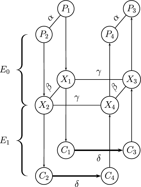
The boomerang attack. Introduced by Wagner [50], the boomerang attack was one of the first techniques to show that non-existence of ‘long’ high-probability differentials is not sufficient to guarantee security with respect to differential-type attacks. Suppose that the cipher E can be decomposed as $E = E_1 \circ E_0$, such that for $E_0$, there exists a differential characteristic $\alpha \xrightarrow {p} \beta$, and for $E_1$, there exists a differential characteristic $\gamma \xrightarrow {q} \delta$, depicted in Fig. 1, where $pq \gg 2^{-n/2}$. Then, one can distinguish E from a random permutation, using Algorithm 1.

Algorithm 1

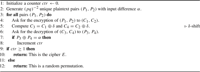
The Boomerang Distinguisher

Fig. 1

The Boomerang Attack

The analysis of the algorithm is as follows. Denote the intermediate values after the partial encryption by $E_0$ of the plaintext $P_j$ by $X_j$, for $1 \le j \le 4$. Let $(P_1,P_2)$ be a plaintext pair such that $P_1 \oplus P_2 = \alpha$. By the differential characteristic of $E_0$, we have

$$\begin{aligned} X_1 \oplus X_2 = \beta , \end{aligned}$$

(1)

with probability p. On the other side, as the ciphertexts satisfy $C_1 \oplus C_3 = C_2 \oplus C_4 = \delta$, by the differential characteristic of $E_1$ we have

$$\begin{aligned} (X_1 \oplus X_3 = \gamma ) \wedge (X_2 \oplus X_4 = \gamma ), \end{aligned}$$

(2)

with probability $q^2$. (We recall that the differential characteristic $\gamma \xrightarrow {q} \delta$ for $E_1$ is identical to the differential characteristic $\delta \xrightarrow {q} \gamma$ for $E_1^{-1}$, in the sense that both count the same set of input/output pairs for $E_1$.) If both Eqs. (1) and (2) hold, then we have

$$\begin{aligned} X_3 \oplus X_4 = (X_3 \oplus X_1) \oplus (X_1 \oplus X_2) \oplus (X_2 \oplus X_4) = \gamma \oplus \beta \oplus \gamma = \beta . \end{aligned}$$

(3)

Therefore, by the differential characteristic of $E_0$, we have $P_3 \oplus P_4 = \alpha$, with probability p. Hence, assuming (somewhat non-carefully, as discussed in [42] and in ‘Appendix A’) that all these events are independent, we have

$$\begin{aligned} \Pr [P_3 \oplus P_4 = \alpha | P_1 \oplus P_2 = \alpha ] = p^2 q^2. \end{aligned}$$

(4)

As we take $1/(pq)^2$ pairs $(P_1,P_2)$, then with a high probability ($=1-e^{-1} \approx 63\%$),³ for at least one of them we obtain $P_3 \oplus P_4 = \alpha$, and hence, the algorithm outputs ‘the cipher E.’ On the other hand, for a random permutation we have $\Pr [P_3 \oplus P_4 = \alpha ] = 2^{-n}$, and hence, the expected number of pairs $(P_1,P_2)$ for which $P_3 \oplus P_4 = \alpha$ holds is $2^{-n} \cdot (pq)^{-2} \ll 1$ (as we assumed $pq \gg 2^{-n/2}$). Thus, with an overwhelming probability, the algorithm outputs ‘random permutation.’

Therefore, the above algorithm indeed allows distinguishing E from a random permutation, using in total $4(pq)^{-2}$ adaptively chosen plaintexts and ciphertexts (in the sequel: ACC).

2.2 The S-box Switch

In [19], Biryukov and Khovratovich showed that in certain cases, the boomerang attack can be improved significantly by ‘bypassing for free’ some operations in the middle of the cipher. One of those cases, called S-box switch, is particularly relevant to our results. Assume that $E=E_1 \circ E_0$, where the last operation in $E_0$ is a layer S of S-boxes applied in parallel (which is the usual scenario in SP networks, like the AES). That is, S divides the state $\rho$ into $\rho =(\rho _1,\rho _2,\ldots ,\rho _t)$ and transforms it to $S(\rho ) = (f_1(\rho _1)||f_2(\rho _2)||\ldots || f_t (\rho _t))$, for t independent (keyed) functions $f_j$. Suppose that the differential characteristics in $E_0,E_1$ are such that in both $\beta$ and $\gamma$, the difference in the part of the intermediate state X that corresponds to the output of some $f_j$ is $\varDelta$. In other words, denoting this part of the intermediate state X by $X_j$, if both characteristics hold then we have

$$\begin{aligned} (X_1)_j \oplus (X_2)_j = (X_1)_j \oplus (X_3)_j = (X_2)_j \oplus (X_4)_j = \varDelta . \end{aligned}$$

In such a case, we have $(X_1)_j=(X_4)_j$ and $(X_2)_j=(X_3)_j$, and hence, if the differential characteristic in the function $(f_j)^{-1}$ holds for the pair $(X_1,X_2)$, then it must hold for the pair $(X_3,X_4)$. Thus, the overall probability of the boomerang distinguisher is increased by a factor of $(q')^{-1}$, where $q'$ is the probability of the differential characteristic in $f_j$.

This ‘switch,’ along with other ‘switches in the middle,’ was a key ingredient in the attack of [19] on the full AES-192 and AES-256. Later on, some of these switches were generalized in the Sandwich attack of [30] for the case of a probabilistic transition in the middle layer and used to attack KASUMI, the cipher of 3 G cellular networks. Recently, a more complete and rigorous analysis of the transition between $E_0$ and $E_1$ was suggested, using the Boomerang Connectivity Table [24] that covers these and related ideas. These developments are described in more detail in ‘Appendix A.’

2.3 The Yoyo Game and Mixture Differentials

In addition to the classical boomerang attack, two more techniques—the yoyo game and mixture differentials—are closely related to our attacks. We describe them very briefly below, but in more detail in the sequel. Our new type of boomerang attacks allows us to unveil a close relation of these two techniques to the boomerang and rectangle techniques, respectively.

The yoyo game. The yoyo technique was introduced by Biham et al. [10] in 1998. Like the boomerang attack, the yoyo game is based on encrypting a pair of plaintexts $(P_1,P_2)$, modifying the corresponding ciphertexts $(C_1,C_2)$ into $(C_3,C_4)$, and decrypting them. However, while the boomerang distinguisher just checks whether the resulting plaintexts $(P_3,P_4)$ satisfy some property, in the yoyo game the process continues: $(P_3,P_4)$ are modified into $(P_5,P_6)$ which are encrypted into $(C_5,C_6)$, those in turn are modified into $(C_7,C_8)$ which are decrypted into $(P_7,P_8)$, etc. The process satisfies the property that all pairs of intermediate values $(X_{2\ell +1},X_{2\ell +2})$ at some specific point of the encryption process satisfy some property (e.g., zero difference in some part of the state). Since for a random permutation, the probability that such a property is satisfied by a sequence of pairs $(X_{2\ell +1},X_{2\ell +2})$ is extremely low, this property can theoretically be used for distinguishing the cipher from a random permutation. Practically, exploiting this property is not so easy, as the adversary does not see the intermediate values $(X_{2\ell +1},X_{2\ell +2})$. Nevertheless, Biham et al. showed that in some specific cases, such a distinguishing is possible and even allows for key recovery [10].

Biham et al. [10] applied the yoyo technique to a 16-round variant of the block cipher Skipjack. Biryukov et al. [20] applied it to attack generic 5-round Feistel constructions, and Rønjom et al. [46] used it to attack reduced-round AES with at most 5 rounds. As the attack of Rønjom et al. [46] is a central ingredient in our attacks on 5-round AES, we recall its details in Sect. 4.

Mixture differentials. The mixture differential technique was presented by Grassi [33]. The technique works in the following setting. Assume that the cipher E can be decomposed as $E = E_1 \circ E_0$, where $E_0$ can be considered as a concatenation of several permutations, i.e., $P=(\rho _1,\rho _2,\ldots ,\rho _t)$ and $E_0(P) = f_1(\rho _1)||f_2(\rho _2)||\ldots || f_t (\rho _t))$, for t independent functions $f_j$. A well-known example of such $E_0$ is 1.5 rounds of AES that can be treated as four parallel super S-boxes (see [26]).

Definition 1

Given a plaintext pair $(P^1,P^2)$, where $P^1=(\rho ^1_1,\ldots ,\rho ^1_t)$ and $P^2=(\rho ^2_1,\ldots ,\rho ^2_t)$ we say that $(P^3,P^4)$, where $P^3=(\rho ^3_1,\ldots ,\rho ^3_t)$ and $P^4=(\rho ^4_1,\ldots ,\rho ^4_t)$ is a mixture counterpart of $(P^1,P^2)$ if for each $1 \le j \le t$, the quartet $(\rho _j^1,\rho _j^2,\rho _j^3,\rho _j^4)$ consists of two pairs of equal values or of four equal values. The quartet $(P^1,P^2,P^3,P^4)$ is called a mixture.

The main observation behind the mixture differential technique is that if $(P^1,P^2,P^3,P^4)$ is a mixture, then the XOR of the corresponding intermediate values $(X^1,X^2,X^3,X^4)$ is zero. Indeed, for each j, as $(\rho _j^1,\rho _j^2,\rho _j^3,\rho _j^4)$ consists of two pairs of equal values, then the same holds for $(f_j(\rho _j^1),f_j(\rho _j^2),f_j(\rho _j^3),f_j(\rho _j^4))$ as well. In particular, $f_j(\rho _j^1) \oplus f_j(\rho _j^2) \oplus f_j(\rho _j^3) \oplus f_j(\rho _j^4)) =0$. As a result, if we have $X^1 \oplus X^3 = \gamma$, then $X^2 \oplus X^4 = \gamma$ holds as well. Now, if there exists a differential characteristic $\gamma \xrightarrow {q} \delta$ for $E_1$, then with probability $q^2$, the corresponding ciphertexts satisfy $C^1 \oplus C^3 = C^2 \oplus C^4 = \delta$.

Grassi [33, 34] applied the technique to mount several attacks on AES with up to 6 rounds. The 5-round attack of Grassi was recently improved in [4] into an attack with overall complexity of $2^{24}$ for full key recovery (or $2^{21.5}$ for recovering 24 bits of the secret key) that is significantly faster than all other known attacks on 5-round AES.

3 The Retracing Boomerang Attack

Our new retracing boomerang framework contains two attack types—a shifting type and a mixing type. In this section, we present these two types and discuss their advantages over the standard boomerang attack and their relation to previous works. In the following sections, we present applications of the new techniques, along with a few variants and extensions.

3.1 The Shifting Retracing Attack

Assumptions. Suppose that the block cipher E can be decomposed as $E = E_{12} \circ E_{11} \circ E_0$, where $E_{12}$ consists of dividing the state into two parts (a left part of b bits and a right part of $n-b$ bits) and applying to them the functions $E_{12}^L,E_{12}^R$, respectively. Furthermore, suppose that for $E_0$, there exists a differential characteristic $\alpha \xrightarrow {p} \beta$, for $E_{11}$, there exists a differential characteristic $\gamma \xrightarrow {q_1}(\mu _L,\mu _R)$, for $E_{12}^L$, there exists a differential characteristic $\mu _L \xrightarrow {q_2^L} \delta _L$, and for $E_{12}^R$, there exists a differential characteristic $\mu _R \xrightarrow {q_2^R} \delta _R$ (see Fig. 2).⁴

Fig. 2

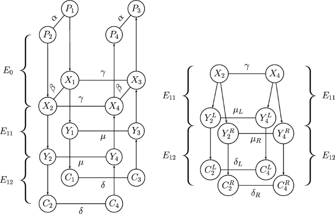
The Retracing Boomerang Framework

In other words, we make the same assumptions as in the boomerang attack, with the additional assumption that $E_1$ can be further decomposed into two sub-ciphers, and that the second sub-cipher has a specific structure. A class of constructions for which this additional assumption holds is SASAS constructions [21], in which $E_{12}$ can be taken to be the last S layer. A specific such example is AES [44], where $E_{12}$ can be taken to be the last 1.5 rounds.

The attack procedure and its analysis. Assuming that $pq_1 q_2^L q_2^R \gg 2^{-n/2}$, the standard boomerang attack can be used to distinguish E from a random permutation, with data complexity of $4(pq_1 q_2^L q_2^R)^{-2}$.

The basic idea of the retracing boomerang attack is to add an artificial $(b-1)$-bit filtering in the middle of the attack procedure. Namely, after encrypting $(P_1,P_2)$ into $(C_1,C_2)$, we first check whether

$$\begin{aligned} C_1^L \oplus C_2^L = 0 \text{ or } \delta _L. \end{aligned}$$

(5)

Only if one of the equalities holds, we continue with the boomerang process. Otherwise, we simply discard the pair $(P_1,P_2)$. See Fig. 3 for the process.

Fig. 3

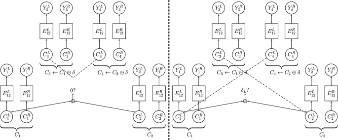
A Shifted Quartet (dashed line represents equality)

This is a surprising move, as the discarded pair may actually be a right pair with respect to the differential characteristic $\alpha \rightarrow \beta$ (i.e., a pair that satisfies the characteristic). Hence, a natural question arises: What do we gain from this filtering?

Note that for any value of $\delta _L$, if Eq. (5) holds, then the two unordered pairs $(C_1^L,C_3^L)$ and $(C_2^L,C_4^L)$ are identical. Hence, if one of these pairs satisfies the differential characteristic $\delta _L \xrightarrow {q_2^L} \mu _L$, then the other one must satisfy it as well. As a result, the probability of the boomerang distinguisher among the examined pairs is increased by a factor of $(q_2^L)^{-1}$ from $(pq_1 q_2^L q_2^R)^2$ to $(pq_1 q_2^R)^2 q_2^L$.

Advantages of the new technique. At first glance, our new variant of the boomerang attack seems completely odd and useless. Note that as the block size of $E_{12}^L$ is b bits, then any possible differential characteristic of $E_{12}^L$ has probability of at least $2^{-b+1}$, and so, the overall probability of the boomerang distinguisher is increased by a factor of at most $2^{b-1}$. On the other hand, our filtering leaves only $2^{-b+1}$ of the pairs, so we either gain nothing (if $q_2^L=2^{-b+1}$) or even lose (otherwise)!

It turns out that there are several advantages to this approach:

1. Improving the signal-to-noise ratio. Recall that the ordinary boomerang attack applies if $pq_1 q_2^L q_2^R \gg 2^{-n/2}$, as otherwise, the probability that $P_3 \oplus P_4 = \alpha$ holds for E is not larger than the respective probability for a random permutation. In the retracing boomerang attack, the probability that $P_3 \oplus P_4 = \alpha$ holds among the examined pairs is increased by a factor of $(q_2^L)^{-1}$, while the probability for a random permutation remains unchanged. As a result, the attack can succeed in cases where the ordinary boomerang attack fails due to insufficient filtering.

Furthermore, the adversary can use the increased gap between the probabilities of the checked event for E and for a random permutation to replace the differential characteristic $\beta \xrightarrow {p} \alpha$ used for the pair $(X_3,X_4)$ in the backward direction with a truncated differential characteristic⁵$\beta \xrightarrow {p'} \alpha '$ of a higher probability $p'$ in which $\alpha '$ specifies the difference in only some part of the bits, while still having a larger probability of the event $P_3 \oplus P_4 = \alpha '$ for E than for a random permutation. An example of this advantage is demonstrated in the attack on 5-round AES presented in Sect. 6.1.

2. Reducing the data complexity. The new attack saves data complexity on the decryption side. Indeed, as decryption is performed only to the pairs that satisfy the filtering condition, the number of decryptions is reduced by a factor of $2^{b-1}$. While usually, the effect of this reduction is not significant as then the encryptions dominate the overall complexity, there are cases in which more queries are made on the decryption side, and in such cases, the data complexity may be significantly reduced. This advantage (like the previous one) is demonstrated in the attack on 5-round AES in Sect. 6.1.

3. Reducing the time complexity. The smaller number of pairs on the decryption side may affect also the time complexity of the attack. This effect is not significant when the attack complexity is dominated by the encryption/decryption of the data. However, in many cases (e.g., where a round is added before the distinguisher and the adversary has to guess some key material in the added round and check whether the condition $P_3 \oplus P_4 = \alpha$ holds), the complexity of the attack is dominated by analysis of the pairs $(P_3,P_4)$. In such cases, the time complexity may be reduced by a factor of $(q_2^L)^{-1}$, as the number of pairs $(P_3,P_4)$ is reduced by this ratio.

Relation to previous works. Our new technique uses several ideas that already appeared in previous works in different contexts. Those include:

• Discarding part of the data before the analysis. The counterintuitive idea of neglecting part of the data appears in various previous works, e.g., in the context of time-memory trade-off attacks on stream ciphers [28] and in the context of conditional linear attacks on DES [15].

• Increasing the probability of the boomerang attack by exploiting dependency between differentials. As we mentioned above, several previous works on the boomerang attack used dependency between differentials, and in particular, situations in which the four inputs to some function in the encryption process are composed of two pairs of equal values, to increase the probability of the boomerang distinguisher (see, e.g., [18, 19, 24, 30]). The closest to our attack is the S-box switch of Biryukov and Khovratovich [19] described in Sect. 2. In all these attacks, the gain is obtained in the transition between the two sub-ciphers $E_0,E_1$. In contrast, the retracing boomerang exploits dependency between the two differentials in the same sub-cipher (by forcing dependency via the artificial filtering).

• Increasing the probability of the boomerang attack by exploiting representation of a sub-cipher as two (or more) functions applied in parallel. Such a probability increase was obtained by Biryukov and Khovratovich [19] in the ladder switch technique, which exploits a subdivision into multiple functions (e.g., a layer of S-boxes) along with dependency between differentials, to increase the probability of the transition between the two sub-ciphers.

• Using quartets of the form (x, x, y, y) to force dependency. This idea was recently used by Grassi in [33, Theorem 4], in the context of the mixture differential attack described in Sect. 2.

Application. An application of the shifting retracing boomerang technique is given in Sect. 6, where it is used to improve the classical boomerang attack of Biryukov [17] on 5-round and 6-round AES.

3.2 The Mixing Retracing Attack

The attack setting. Recall that the shifting retracing boomerang attack increases the probability of the boomerang distinguisher by forcing equality between the unordered pairs $(C_1^L,C_2^L)$ and $(C_3^L,C_4^L)$ that enter $(E_{12}^L)^{-1}$. Such an equality can be forced in an alternative way, without inserting an artificial filtering.

Instead of working with the same shift $\delta$ for all ciphertexts, one may shift each ciphertext pair $(C_1,C_2)$ by $(C_1^L \oplus C_2^L, 0)$, thus obtaining the ciphertexts

$$\begin{aligned} C_3 = (C_3^L,C_3^R) = \left( C_1^L \oplus (C_1^L \oplus C_2^L), C_1^R \oplus 0\right) = (C_2^L,C_1^R), \end{aligned}$$

and (similarly) $C_4=(C_1^L,C_2^R)$, see Fig. 4. In such a case, the unordered pairs $(C_1^L,C_3^L)$ and $(C_2^L,C_4^L)$ are equal, and hence, we gain a factor of $(q_2^L)^{-1}$, like in the shifting retracing attack. Furthermore, in the right part we have $C_1^R=C_3^R$ and $C_2^R=C_4^R$, and thus, we gain also a factor of $(q_2^R)^{-2}$ (as both characteristics in $E_{12}^R$ hold trivially with probability 1). This results in a total gain of $(q_2^L)^{-1} (q_2^R)^{-2}$.

Fig. 4

A Mixture Quartet of Ciphertexts (a dashed line means equality)

Relation to ‘yoyo tricks with AES.’ Interestingly, in the special case of the AES, the mixing described here is exactly the core step of the yoyo attack of Rønjom et al. [46] (presented in detail in Sect. 4). Hence, this type of retracing boomerang is not entirely novel, but rather generalizes and presents a new viewpoint on the yoyo attack of Rønjom et al.

Application. The attacks on 5-round AES with known and secret S-boxes, presented in Sects. 4 and 5, respectively, are applications of the mixing retracing boomerang technique.

3.3 Comparison Between the Two Types of Retracing Boomerang

At a first glance, it seems that the mixing retracing attack is clearly better than the shifting retracing attack presented above. Indeed, it obtains an even larger gain in the probability of the distinguisher, while not discarding ciphertext pairs! However, there are several advantages of the shifting variant that make it more beneficiary in various scenarios:

• Using structures. As is described in ‘Appendix A,’ a central technique for extending the basic boomerang attack is adding a round at the top of the distinguisher, using structures. This technique can be combined with the shifting retracing technique, as follows. First, the adversary performs the ordinary boomerang attack with structures (i.e., encrypts structures of plaintexts, shifts all ciphertexts by $\delta$ and decrypts the resulting ciphertexts), and then she checks the artificial filtering together with the condition on $P_3,P_4$, since both can be checked simultaneously using a hash table. As a result, the data complexity remains the same as in the ordinary boomerang attack (given the use of structures), while the retracing boomerang leads to an improvement in the signal-to-noise ratio, which can be translated to a reduction in the data complexity, as described above.

  For mixing retracing, such a combination is impossible, since each ciphertext pair $(C_1,C_2)$ has to be modified by its own shift $(C_1^L \oplus C_2^L,0)$, and so, one cannot shift entire structures at a whole. Therefore, the reduction of data complexity by using structures cannot be obtained.

  A similar advantage of the shifting variant is the ability to combine it with an extension of the boomerang attack by adding a round at the bottom (i.e., after the distinguisher), as we demonstrate in our attack on 6-round AES in Sect. 6.3.

• Combination with $E_{11}$. In the mixing variant, since the output difference for $(E_{12}^L)^{-1}$ (namely $(C_1)^L \oplus (C_2)^L$) is arbitrary and changes between different pairs, in most cases there is no good way to combine a differential characteristic of $(E_{12}^L)^{-1}$ with a differential characteristic of $(E_{11})^{-1}$. Indeed, in the yoyo attack of [46] on 5-round AES, this part of the attack succeeds simply because $E_{11}$ is empty. It seems that while the mixing retracing technique can be applied also in cases where $E_{11}$ is nonlinear (and, in particular, non-empty), it will usually (or even almost always) be inferior to the shifting retracing boomerang in such cases.

• Construction of ‘friend pairs.’ An important ingredient in many boomerang attacks is ‘friend pairs,’ which are pairs that are attached to specific pairs in such a way that if some pair satisfies a desired property then all its ‘friend pairs’ satisfy the same property as well. (Such pairs are used in most attacks in this paper; see Sect. 8 for a discussion.) While both types of the retracing boomerang attack allow constructing several ‘friend pairs’ for each pair, the number of pairs in the shifting variant is significantly larger, which makes it advantageous in some cases.

The names of the attacks. The shifting type of the retracing boomerang is named this way since it preserves the $\delta$-shift of the original boomerang attack and uses the filtering to enhance the probability of the original boomerang process. The mixing type is named this way since it replaces the $\delta$-shift by a mixing procedure, like the one used in mixture differentials [33].

3.4 Another Variant of the Shifting Retracing Boomerang Attack

We conclude this section with another variant of the shifting retracing boomerang attack, which can be combined with the standard variant, as is described below. In this variant, instead of introducing an artificial filtering on the ciphertext side, we introduce such a filtering on the plaintext side.

The attack setting. In this variant, we suppose that E can be decomposed as $E = E_1 \circ E_{02} \circ E_{01}$, where $E_{01}$ consists of dividing the state into two parts (a left part of b bits and a right part of $n-b$ bits) and applying to them the functions $E_{01}^L,E_{01}^R$. Furthermore, we suppose that for $E_{01}^L$, there exists a differential characteristic $\alpha _L \xrightarrow {p_1^L} \mu _L$, for $E_{01}^R$, there exists a differential characteristic $\alpha _R \xrightarrow {p_1^R} \mu _R$, for $E_{02}$, there exists a differential characteristic $\mu \xrightarrow {p_2} \beta$, and for $E_{1}$, there exists a differential characteristic $\gamma \xrightarrow {q} \delta$ (see Fig. 8).

In this scenario, we can introduce an artificial filtering on the plaintext side. We first perform the ordinary boomerang process, and then, before checking whether the equation $P_3 \oplus P_4 = \alpha$ holds, we first check whether

$$\begin{aligned} P_1^L \oplus P_3^L = 0 \text{ or } \alpha _L, \end{aligned}$$

(6)

and otherwise, we discard the pair $(P_1,P_2)$. Like in the shifting retracing attack, if Eq. (6) holds, then the unordered pairs $(P_1^L,P_2^L)$, $(P_3^L,P_4^L)$ are equal. Hence, if the pair $(P_1,P_2)$ satisfies the differential characteristic of $E_{01}^L$ in the forward direction, then the pair $(E_{01}^L(P_3),E_{01}^L(P_4))$ must satisfy the differential characteristic of $E_{01}^L$ in the backward direction. This increases the probability of the boomerang distinguisher by a factor of $p_1^L$, at the expense of discarding all but a fraction $2^{1-b}$ of the plaintext pairs.

Advantages. This variant of retracing boomerang is less advantageous than the shifting variant, as it does not reduce the data complexity of the attack. (Indeed, the artificial filtering is performed only after the data are collected.)⁶ The main advantage of this attack is improving the signal-to-noise ratio, which allows applying this attack in cases where the ordinary boomerang attack cannot be applied. Another possible advantage is reducing the time complexity, as was described above for the shifting retracing boomerang attack.

Combining with the shifting retracing attack. If the cipher E has both the structure of the shifting retracing attack and of the current attack simultaneously (i.e., if both $E_0$ and $E_1$ can be decomposed into two sub-ciphers of the prescribed form), then the two techniques can be combined by performing two artificial filterings—one on the ciphertext side (before the decryption) and one on the plaintext side (after the decryption). The analysis is a straightforward generalization of the analysis presented above.

4 Retracing Boomerang Attack on 5-Round AES

Our first application of the retracing boomerang framework is an improved attack on 5-round AES, which allows recovering the full secret key with data complexity of $2^{15}$, time complexity of $2^{16.5}$, and memory complexity of $2^9$. The attack was fully implemented and verified experimentally. Since our attack is based on central components of the yoyo attack of Rønjom et al. [46] on 5-round AES (which can be viewed as a mixing retracing boomerang attack, as was shown in Sect. 3.2), we begin this section with describing the structure of the AES and presenting the attack of [46]. Then we present our attack, its analysis, and its experimental verification.

4.1 Brief Description of the AES and Notations

The Advanced Encryption Standard (AES) [44] is a substitution-permutation (SP) network which has 128-bit plaintexts and 128-, 192-, or 256-bit keys. Since the descriptions of all attacks we present in this paper are independent of the key schedule, we do not differentiate between these variants.

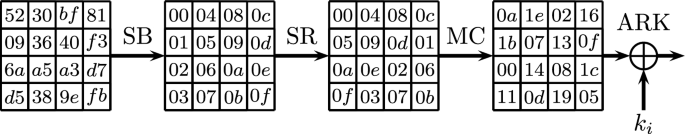
The 128-bit internal state of AES is treated as a byte matrix of size 4x4, where each byte represents a value in $GF(2^8)$. An AES round (described in Fig. 5) applies four operations to this state matrix:

• SubBytes (SB)—applying the same 8-bit to 8-bit invertible S-box 16 times in parallel on each byte of the state,

• ShiftRows (SR)—cyclically shifting the i’th row by i bytes to the left,

• MixColumns (MC)—multiplication of each column by a constant 4x4 matrix over the field $GF(2^{8})$, and

• AddRoundKey (ARK)—XORing the state with a 128-bit subkey.

An additional AddRoundKey operation is applied before the first round, and in the last round the MixColumns operation is omitted. The number of rounds is between 10 and 14, depending on the key length. We omit the key schedule, as it does not affect the description of our attacks.

Fig. 5

An AES Round

The bytes of each state of AES are numbered $0,1,\ldots ,15$, where for $0 \le i,j \le 3$, the j’th byte in the i’th row is numbered $i+4j$ (see the state after SB in Fig. 5). We always consider 5-round AES, where the MixColumns operation in the last round is omitted. The rounds are numbered 0, 1, 2, 3, 4. The subkeys are numbered $k_{-1},k_0,\ldots ,k_4$, where $k_{-1}$ is the secret key XORed to the plaintext at the beginning of the encryption process. We denote by W, Z,  and X the intermediate states before the MixColumns operation of round 0, at the input to round 1 and before the MixColumns operation of round 2, respectively. The j’th byte of a state or a key $X_i$ is denoted by $X_{i,j}$ or by $(X_{i})_{j}$. When several bytes $j_1,\ldots ,j_\ell$ are considered simultaneously, they are denoted by $X_{i,\{j_1,\ldots ,j_\ell \}}$ or by $(X_{i})_{\{j_1,\ldots ,j_\ell \}}$.

The term ‘$\ell$’th shifted column’ (resp., ‘$\ell$’th inverse shifted column’) refers to the result of applying SR (resp., SR$^{-1}$) to the $\ell$’th column. For example, the 0’th shifted column consists of bytes 0, 7, 10, 13, and the 0’th inverse shifted columns consists of bytes 0, 5, 10, 15. We also denote by SR(j) (resp., $SR^{-1}(j)$) the byte position to which byte j is transformed by SR (resp., SR$^{-1}$).

When considering differences between the encryption processes of a pair of plaintexts, we say that a component (e.g., a byte or a column) at some stage of the encryption process is active if the difference in that component is nonzero. Otherwise, we call the component passive. Finally, we say that some values $x_1,x_2,\ldots ,x_m$ ‘sum up to zero’ if $x_1 \oplus x_2 \oplus \ldots \oplus x_m = 0$.

4.2 The Yoyo Attack of Rønjom et al. on 5-Round AES

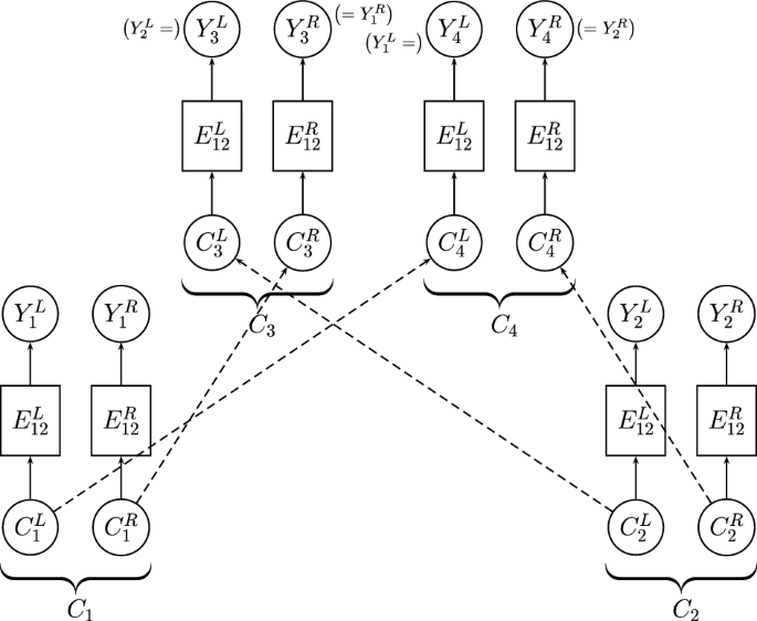
The idea behind the attack. The attack decomposes 5-round AES as $E=E_{12} \circ E_{11} \circ E_0$, where $E_0$ consists of the first 2.5 rounds, $E_{11}$ is the MC operation of round 2, and $E_{12}$ consists of rounds 3 and 4. For $E_0$ in the forward direction, the adversary uses a truncated differential characteristic whose input difference is zero in three inverse shifted columns, and whose output difference is zero in a single shifted column. The probability of the characteristic is $4 \cdot 2^{-8}=2^{-6}$, since it holds if and only if the output difference of the active column in round 0 is zero in at least one byte. For $E_{12}$ in the backward direction, recall that 1.5 rounds of AES can be represented as four 32-bit to 32-bit super S-boxes applied in parallel (see [26]). For each ciphertext pair $(C_1,C_2)$, the adversary modifies it into one of its mixture counterparts (see Definition 1) with respect to the division into super S-boxes, calls the new ciphertext pair $(C_3,C_4)$, and asks for its decryption. Due to the mixture construction, the four outputs of each super S-box are composed of two pairs of equal values, and hence, the four corresponding inputs to the super S-boxes sum up to 0. As MC is a linear operation, this implies that $X_1 \oplus X_2 \oplus X_3 \oplus X_4=0$. Therefore, with probability $2^{-6}$, the difference $X_3 \oplus X_4$ equals zero in a shifted column. This, in turn, implies that the difference $Z_3 \oplus Z_4$ equals zero in an inverse shifted column (i.e., one of the four quartets of bytes: (0, 5, 10, 15), (1, 4, 11, 14), (2, 5, 8, 15), (3, 6, 9, 12)).

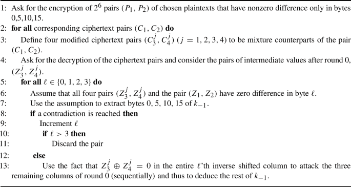
At this point, the adversary would like to attack bytes 0, 5, 10, 15 of the subkey $k_{-1}$, using the fact that in one of the bytes of the first column, we have $Z_3 \oplus Z_4 =0$. However, this information provides only an 8-bit filtering, while 32 subkey bits are involved. In order to improve the filtering, the authors of [46] construct ‘friend pairs’ of the pair $(Z_3,Z_4)$, such that if we have $Z_3 \oplus Z_4 =0$ in byte $\ell$, then the same holds for all friend pairs. (This is achieved by taking several mixture counterparts of the ciphertext pair $(C_1,C_2)$.) The resulting attack algorithm (of [46]) is given in Algorithm 2.

Algorithm 2

Rønjom et al.’s Yoyo Attack on 5-Round AES

Analysis of the attack. The data complexity of the attack is about $2^9$, since for each of $2^6$ pairs $(P_1,P_2)$, the adversary decrypts four ciphertext pairs $(C^j_3,C^j_4)$. The time and memory complexities are dominated by the attack on $k_{-1}$ in Step 7. In a naive application, this attack requires about $2^{32}$ operations for each pair $(P_1,P_2)$ and each value of $\ell \in \{0,1,2,3\}$, and thus, the overall time complexity of the attack is about $2^{32} \cdot 2^6 \cdot 4 = 2^{40}$. The authors of [46] managed to improve the overall complexity to $2^{31}$, using a careful analysis of round 0, including exploitation of the specific matrix used in MC. We do not present this part of the attack, as it can be replaced by a simpler and stronger tool, as we describe below. To summarize, the data complexity of the attack is $2^9$ adaptively chosen plaintexts and ciphertexts, the memory complexity is $2^9$ and the time complexity is $2^{31}$ encryptions.

4.3 A Simple Improvement of the Yoyo Attack on 5-round AES

A simple improvement of the attack of Rønjom et al. is to use a meet-in-the-middle (MITM) procedure to attack bytes 0, 5, 10, 15 of $k_{-1}$ in Step 7.

Using our previously introduced notations, W is the intermediate encryption value before the MC operation of round 0 and $W_m$ is the value in byte m. W.l.o.g. we consider the case $\ell =0$, and recall that by the structure of AES, byte 0 in the input to round 1 satisfies

$$\begin{aligned} Z_0 = 02_x \cdot W_0 \oplus 03_x \cdot W_1 \oplus 01_x \cdot W_2 \oplus 01_x \cdot W_3. \end{aligned}$$

(7)

In the MITM procedure, the adversary guesses bytes 0, 5 of $k_{-1}$, computes the value

$$\begin{aligned} 02_x \cdot (W^j_3)_0 \oplus 03_x \cdot (W^j_3)_1 \oplus 02_x \cdot (W^j_4)_0 \oplus 03_x \cdot (W^j_4)_1 \end{aligned}$$

(8)

for $j=1,2,3$, and stores the concatenation of these values (i.e., a 24-bit value) in a sorted table. Then she guesses bytes 10, 15 of $k_{-1}$, computes the value

$$\begin{aligned} 01_x \cdot (W^j_3)_2 \oplus 01_x \cdot (W^j_3)_3 \oplus 01_x \cdot (W^j_4)_2 \oplus 01_x \cdot (W^j_4)_3 \end{aligned}$$

(9)

for $j=1,2,3$, and checks for a match in the table (which is, of course, equivalent to the condition $(Z^j_3)_0 = (Z^j_4)_0$ for $j=1,2,3$). As this condition is a 24-bit filtering, about $2^{32} \cdot 2^{-24} = 2^8$ suggestions for bytes 0, 5, 10, 15 of $k_{-1}$ remain, and those can be checked using the conditions $(Z^4_3)_0 = (Z^4_4)_0$ and $(Z_{1})_0 = (Z_{2})_0$.

The data complexity of the attack remains $2^9$. The time complexity is reduced to $2^6 \cdot 4 \cdot 2^{16} = 2^{24}$ operations, where each operation is roughly equivalent to a computation of one AES round in a single column for 6 plaintexts, or a total of less than $2^{23}$ encryptions.

It seems that the use of MITM increases the memory complexity of the attack to about $2^{16}$. However, one can maintain the memory at $2^9$ using the dissection technique [27]. (See, e.g., [4] for similar applications of dissection.) Therefore, the time complexity of the attack is reduced to $2^{23}$ encryptions, while the data and memory complexities remain unchanged at $2^9$.

4.4 An Attack on 5-Round AES with Overall Complexity of $2^{16.5}$

We now show how one can reduce the time complexity of the attack described above to $2^{16.5}$, at the expense of increasing the data complexity to about $2^{15}$.

The idea behind the attack is to enhance the MITM procedure, such that on each of the two sides, the number of possible key values is reduced to $2^8$ (instead of $2^{16}$). The reduction is obtained using two methods:

Constructing an extra equation by a specific choice of plaintexts. In order to reduce the number of possible values of $k_{-1,\{0,5\}}$, we choose plaintext pairs with nonzero difference only in bytes 0, 5. For such pairs, the condition $(Z_{1})_0 = (Z_{2})_0$ simplifies into

$$\begin{aligned} 02_x \cdot (W_1)_0 \oplus 03_x \cdot (W_1)_1 = 02_x \cdot (W_2)_0 \oplus 03_x \cdot (W_2)_1, \end{aligned}$$

(10)

as bytes 2, 3 of W cancel out. This equation depends only on the plaintexts and on bytes 0, 5 of $k_{-1}$, and since it is an 8-bit filtering, it leaves only $2^8$ possible values of $k_{-1,\{0,5\}}$. In order to detect these $2^8$ candidates efficiently, we make our choice of plaintexts even more specific.

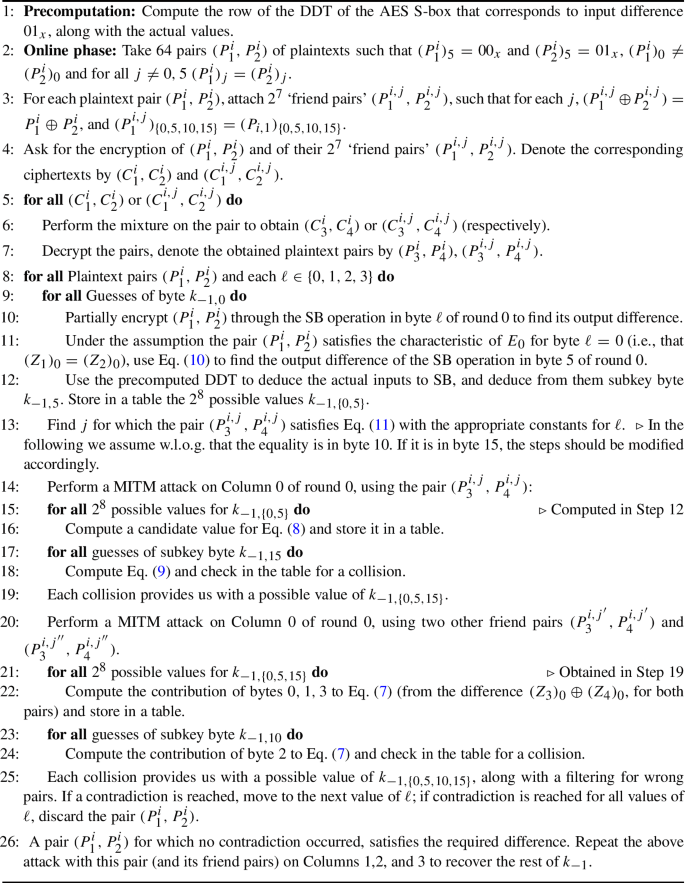
We choose only pairs of plaintexts $(P_1,P_2)$ that satisfy $(P_1)_5 \oplus (P_2)_5 = 01_x$. In addition, as a precomputation phase we compute the row of the Difference Distribution Table (DDT) of the AES S-box that corresponds to input difference $01_x$ and store it in memory, where each output difference is stored along with the value(s) that lead to it.⁷

As a result, for each pair $(P_1,P_2)$ and for each guess of $k_{-1,0}$, we can use Eq. (10) to compute the output difference of the SB operation in byte 5. As the input difference is fixed to be $01_x$, we can use the precomputed row of the DDT to find the inputs to that SB operation by a single table lookup, and hence, to instantly retrieve the possible values of $k_{-1,5}$ that correspond to the guessed value of $k_{-1,0}$.

This process allows us to compute the $2^8$ possible values of $k_{-1,\{0,5\}}$ in about $2^{8}$ simple operations for each pair.

Eliminating a key byte from the equation by using multiple ‘friend pairs.’ In order to reduce the number of possible values of $k_{-1,\{10,15\}}$, we attach to each plaintext pair $(P_1,P_2)$ multiple ‘friend pairs,’ such that if $(P_1,P_2)$ satisfies the differential characteristic of $E_0$, then all ‘friend pairs’ satisfy the same characteristic as well. We perform the boomerang process for all ‘friend pairs’ together with the original pairs, obtaining many pairs $(P^j_3,P^j_4)$.

We note that the method for constructing ‘friend pairs’ used in [46] (namely using several mixtures of the ciphertext pair $(C_1,C_2)$) can supply only up to 15 ‘friend pairs’ for a given plaintext pair $(P_1,P_2)$. In order to obtain many more ‘friend pairs,’ we construct them on the plaintext side, by changing the value of both plaintexts in some of the ‘non-active’ bytes (namely bytes 1,2,3,4,6,7,8,9,11, 12,13,14). This allows us to attach up to $2^{96}$ ‘friend pairs’ to a given pair. (Of course, we don’t need such a large amount. As is shown below, about 128 ‘friend pairs’ are sufficient.)

We choose one ‘friend pair’ for which we have

$$\begin{aligned} (P^j_3)_{10} \oplus (P^j_4)_{10} = 0 \qquad \text{ or } \qquad (P^j_3)_{15} \oplus (P^j_4)_{15} = 0. \end{aligned}$$

(11)

Assume w.l.o.g. that the equality holds in byte 10. We perform the MITM procedure presented above with the single pair $(P^j_3,P^j_4)$. Note that the first step provided us with $2^8$ possible values for $k_{-1,\{0,5\}}$. Hence, in the MITM attack there are only $2^8$ possible values for Eq. (8). On the other hand, by the choice of the pair, there is a zero difference in byte 2 before the MC operation, and thus, the subkey byte $k_{-1,10}$ cancels out from the expression (9). As a result, this expression depends on a single key byte, and thus, has only $2^8$ possible values, just like Eq. (8). Thus, the MITM procedure requires about $2^{9}$ simple operations and (as the data provides an 8-bit filtering) leaves $2^8$ suggestions for subkey bytes $k_{-1,\{0,5,15\}}$. Finally, we can take any other couple of ‘friend pairs’ and recover the unique value of $k_{-1,\{0,5,10,15\}}$ by another MITM procedure in which one side computes the contribution of bytes 0, 1, 3 to Eq. (10) (applied for the difference $(Z_3)_0 \oplus (Z_4)_0$) and the other side computes the contribution of byte 2, as on each side there are about $2^8$ possible values.

Therefore, the complexity of the MITM attack on $k_{-1,\{0,5,10,15\}}$ is reduced to about $2^8$ operations for each pair $(P_1,P_2)$ and each value of $\ell$, or a total of about $2^{16}$ operations. As for the data complexity, in order to have a friend pair that satisfies Eq. (11) with a high probability, we have to take about $2^7$ friend pairs for each of the $2^6$ pairs $(P_1,P_2)$. Hence, the total data complexity is increased to about $2^{15}$. A more precise analysis is given below.

Attack algorithm. The algorithm of our improved attack on 5-round AES is given in Algorithm 3.

Algorithm 3

Our Improved Retracing Boomerang Attack on 5-Round AES

Attack analysis. The attack succeeds if the data contains a pair that satisfies the truncated differential characteristic of $E_0$ (i.e., leads to a zero difference in at least one byte in the active column in round 0), and in addition, for one of the ‘friend pairs’ of that pair, the corresponding plaintext pair $(P^{i,j}_3,P^{i,j}_4)$ has zero difference in either byte 10 or 15. With 64 plaintext pairs and 128 ‘friend pairs’ for each pair, each of these events occurs with probability of about $1-e^{-1} \approx 0.63$, and hence, under standard randomness assumptions, the success probability of the attack is about $0.63^2 \approx 0.4$. This probability can be significantly increased by increasing the number of pairs we start with and the number of their ‘friend pairs.’ For example, with 128 plaintext pairs and 128 friend pairs for each of them, the expected success probability is $(1-e^{-2})(1-e^{-1}) \approx 0.54$.

We note that the success probability can be further increased by exploiting other ways to cancel terms in Eq. (9). For example, if for some $j,j'$, the unordered pairs $\{(P^{i,j}_3)_{10},(P^{i,j}_4)_{10}\}$ and $\{(P^{i,j'}_3)_{10},(P^{i,j'}_4,)_{10}\}$ are equal, then we can use the XOR of Eq. (9) for both pairs to cancel out the effect of subkey byte $k_{-1,10}$ on the equation. This allows us to apply the efficient MITM attack described above also in cases where no ‘friend pair’ of $(P_1^i,P_2^i)$ satisfies Eq. (11), thus increasing the success probability of the attack. Our analysis shows that under standard randomness assumptions, for the same amount of 64 initial pairs and 128 ‘friend pairs’ for each pair considered above, this improvement increases the success probability of the attack from 0.4 to about 0.5.

The data complexity of the attack, for the success probability 0.4 computed above, is $2 \cdot 2^6 \cdot 2^7 = 2^{14}$ chosen plaintexts and $2^{14}$ adaptively chosen ciphertexts. We note that the amount of chosen plaintexts can be reduced by considering two structures of 8 plaintexts each (where in the first structure we have $(P_1^i)_{5}=00_x$ and $(P_1^i)_{0}$ assumes 8 different values, and in the second structure we have $(P_2^i)_{5}=01_x$ and $(P_2^i)_{0}$ assumes 8 different values) and taking the 64 pairs $(P_1^i,P_2^i)$ composed of one plaintext in each structure. (In such a case, the ‘friend pairs’ are also taken in structures obtained by XORing the same value to all elements in the two initial structures.) This reduces the data complexity to slightly more than $2^{14}$ adaptively chosen plaintexts and ciphertexts (as the number of encrypted plaintexts is negligible with respect to the number of decrypted ciphertexts). On the other hand, this slightly reduces the success probability of the attack, due to dependencies between the examined pairs $(P_1^i,P_2^i)$, as demonstrated in the next subsection. To conclude, with data complexity of $2^{15}$ adaptively chosen plaintexts and ciphertexts we obtain success probability of more than $50\%$.

The memory complexity of the attack is no more than $2^9$ 128-bit memory cells, like in the yoyo attack of Rønjom et al. [46].

As for the time complexity, it is dominated by several steps that consist of about $2^{16}$ simple operations each. The comparison of these operations to AES encryptions is problematic, and hence, we adopt a common strategy of counting the number of S-box applications and dividing it by 80, which is the number of S-boxes in 5-round AES. In addition to the $2^{14}+2^{11}$ full encryptions of Steps 2–8, the number of S-box evaluations (or their equivalent) is as follows: Step 10 takes $2 \cdot 2^{16}$ S-box evaluations, Steps 11–12 take $2\cdot 2^{16}$ S-box evaluations, Steps 15–16 take $4\cdot 2^{16}$ S-box evaluations, and $2\cdot 2^{16}$ in Steps 17–18. Steps 20–24 take $16 \cdot 2^{16}$ S-box evaluations. Step 26 repeats three times (for three columns) a process that takes $24 \cdot 2^{16}$, i.e., a total of $72 \cdot 2^{16}$. Hence, the total time complexity is $98 \cdot 2^{16}$ which is less than $2^{16.5}$ 5-round AES computations.

Fig. 6

Attack Success Probability

We conclude that our 5-round attack requires $2^{15}$ adaptively chosen plaintexts and ciphertexts, $2^{9}$ memory and $2^{16.5}$ time, and recovers the full secret key with success probability of more than $50\%$.

4.5 Experimental Verification

To verify the success probability of our attack computed above, we implemented two variants of the 5-round attack. The first variant uses up to 128 independent plaintext pairs. The second variant uses two structures, one of 8 plaintexts and another of 16 plaintexts, to create a total of 128 plaintext pairs. For each pair $(P_1^i,P_2^i)$, we generated 128 friend pairs. We ran the attack on 500 different randomly generated keys. For each success of the attack, we saved the number of pairs we had to try before finding the key. Then we extracted from this data the success probability of the attack, as a function of the amount of available data. Figure 6 shows this success probability, as a function of the number of plaintext pairs, up to a maximum of 128 pairs.

It can be seen that the success probability is slightly lower than the probability predicted by the above analysis. In particular, for 64 initial pairs, the success probability is slightly higher than 0.3 (rather than the predicted 0.4). We conjecture that the deviation from the theoretical estimate occurs due to dependency issues, but leave this small discrepancy for further research. Anyway, for data complexity of $2^{15}$, the experimental success probability is well above $50\%$.

The source code used in the experiments, along with the raw data, can be found at https://github.com/eyalr0/AES-Cryptoanalysis.

5 Improved Attack on 5-Round AES with a Secret S-box

In [48], Tiessen et al. initiated the study of AES with a secret S-box, namely a variant of AES in which the SB operation is replaced by a key-dependent S-box. They showed that 5 rounds of the new variant can be broken with complexity of $2^{40}$ and 6 rounds can be broken with complexity of $2^{90}$, using variants of the Square attack on AES [44]. In the last years, seven more papers analyzed 5-round variants of AES with a secret S-box: in [25, 36, 47] using the Square attack, in [35, 36] using impossible differentials, in [32] using impossible differentials and the multiple-of-n property, in [6] using the yoyo technique, and in [1] using the exchange property. The best currently known result was obtained by Bardeh and Rønjom [6]—data complexity of $2^{32}$ adaptively chosen plaintexts and ciphertexts and time complexity of $2^{31}$ operations (in addition to generating the data).

In this section we use the retracing boomerang technique to devise an attack on 5-round AES with a secret S-box with a complexity of $2^{25.8}$ in the adaptively chosen plaintext and ciphertext model. Like the attacks of [6, 32, 35, 47], our attack recovers the secret key, without fully recovering the secret S-box. (Actually, we recover the S-box up to an invertible affine transformation in $(GF(2))^8$; as our attack is of a differential nature, it cannot distinguish between secret S-boxes that differ by such transformations.) On the other hand, it applies even against a stronger variant in which MC is also replaced by a key-dependent MDS transformation (see [26]) applied on each column. Among the previous attacks, only the Square attack of Tiessen et al. [48] applies to this variant and can break it with complexity of $2^{40}$.

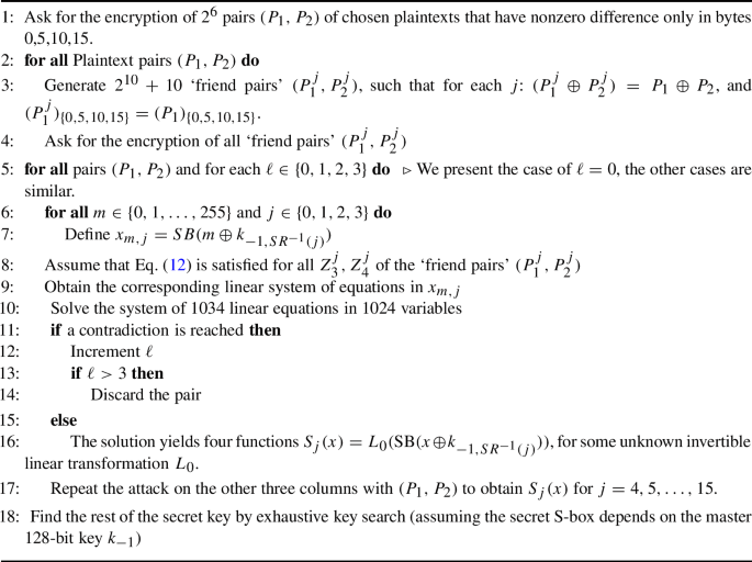
Our attack uses the same retracing boomerang framework as our attack on 5-round AES. Namely, we start with plaintext pairs $(P_1,P_2)$ with difference only in bytes 0, 5, 10, 15, and for each such pair, we modify the corresponding ciphertext pair $(C_1,C_2)$ into one of its mixture counterparts, which we denote by $(C_3,C_4)$, and ask for its decryption. We know that with probability $2^{-6}$, the corresponding pair $(Z_3,Z_4)$ of intermediate values at the input of round 1 has zero difference in an inverse shifted column (e.g., in bytes 0, 5, 10, 15). (Note that this part does not use the specific structure of SB or of MC and, hence, can be applied also to a variant of AES with key-dependent SB and MC operations.) Our goal now is to use this knowledge to attack round 0, as the attack we used for 5-round AES heavily relies on the fact that the S-box is known to the adversary.

Partial recovery of the secret S-box. To attack round 0, we use the strategy proposed in the structural attack of Biryukov and Shamir on SASAS [21], that was already used against AES with a secret S-box in [48], albeit inside the framework of the Square attack. Assume w.l.o.g. that the retracing boomerang predicts a zero difference in byte 0 of the state Z, i.e., yields the equation $(Z_3)_0 \oplus (Z_4)_0 = 0$. (In the actual attack, if the procedure with byte 0 leads to a contradiction, the adversary has to perform it again with bytes 1, 2, 3.) By Eq. (7), we can rewrite this equation as

$$\begin{aligned} \begin{aligned} 0 = (Z_3)_0 \oplus (Z_4)_0 =&02_x \cdot ((W_3)_0 \oplus (W_4)_0) \oplus 03_x \cdot ((W_3)_1 \oplus (W_4)_1) \\&\oplus 01_x \cdot ((W_3)_2 \oplus (W_4)_2) \oplus 01_x \cdot ((W_3)_3 \oplus (W_4)_3). \end{aligned} \end{aligned}$$

(12)

Note that each of the values $(W_3)_j$ has the form $\textrm{SB}(P_3 \oplus k_{-1,j'})$, where for $j=0,1,2,3$, $j'=\textrm{SR}^{-1}(j)$ takes the value 0, 5, 10, 15, respectively. Therefore, if we define $4 \cdot 256 = 1024$ variables $x_{m,j} = \textrm{SB}(m \oplus k_{-1,j'})$ (for $m=0,1,\ldots ,255$ and $j' = 0,1,2,3$), then each plaintext pair $(P_1,P_2)$ for which the corresponding intermediate values $(Z_3,Z_4)$ satisfy

$$\begin{aligned} (Z_3)_0 \oplus (Z_4)_0 = 0, \end{aligned}$$

(13)

provides us with a linear equation in the variables $\{x_{m,j}\}$.

In order to recover the variables $\{x_{m,j}\}$ by solving a system of linear equations, we need many pairs $(Z_3,Z_4)$ that satisfy Eq. (13) simultaneously. We obtain these pairs by attaching about⁸$2^{10}$ ‘friend pairs’ to each original pair $(P_1,P_2)$, like we did in the attack on 5-round AES in Sect. 4. Hence, we start with $2^6$ pairs $(P_1,P_2)$, and for each pair and about $2^{10}$ friend pairs we perform the mixing retracing boomerang process and use each of the pairs to obtain a linear equation in the variables $\{x_{m,j}\}$. (This part of the attack has to be repeated for $\ell =0,1,2,3$, as each value of $\ell$ leads to different equations. The equations presented above correspond to $\ell =0$.) Then, we recover as many as we can of the variables $\{x_{m,j}\}$ by solving a system of linear equations. We take a bit more than $2^{10}$ friend pairs for each pair in order to obtain extra filtering, which allows us to efficiently discard pairs $(P_1,P_2)$ that do not satisfy the boomerang property.

As was shown in [48], the equations do not allow determining the variables $\{x_{m,j}\}$ (and thus, the secret S-box) completely. Indeed, as our basic Eq. (12) represents differences and not actual values, it is invariant under composition of the secret S-box with an invertible linear transformation over $(GF(2))^8$. Thus, the best we can obtain at this stage is four functions $S_0,S_1,S_2,S_3$, such that

$$\begin{aligned} S_j(x) = L_0(\textrm{SB}(x \oplus k_{-1,j'})), \end{aligned}$$

for some unknown invertible linear transformation $L_0$. In addition, by repeating the attack for three other columns in round 0 (using the fact that for a pair $(P_1,P_2)$ that satisfies the boomerang property, an entire inverse shifted column of $Z_3 \oplus Z_4$ equals zero), we obtain the S-boxes $S_j(x)$ for all $j \in \{0,1,\ldots ,15\}$, albeit with multiplication by a different matrix $L_t$ in all the S-boxes of (inverse shifted) $\textrm{Column}(t)$.

Recovering the secret key. While this information does not recover the S-box completely, it does allow us to recover the secret key $k_{-1}$, up to 256 possible values. This is done in two steps.

First, for each $j' \in \{1,2,3\}$ we can easily recover $\bar{k}_{j'} = k_{-1,0} \oplus k_{-1,j'}$ in time $2^8$, as $\bar{k}_{j'}$ is the unique value of c such that $S_j(x) = S_0(x \oplus c)$ for all x. In a similar way, we can recover each inverse shifted column of $k_{-1}$ up to 256 possible values (e.g., to find the values $k_{-1,1} \oplus k_{-1,s}$ for $s \in \{6,11,12\}$ by attacking Column 3). This already reduces the number of possible values of $k_{-1}$ to $2^{32}$.

Second, we find the differences $k_{-1,0} \oplus k_{-1,j}$ for $j=1,2,3$ by taking several quartets of values $(x_1,x_2,x_3,x_4)$ such that $S_0(x_1) \oplus S_0(x_2) \oplus S_0(x_3) \oplus S_0(x_4)=0$ and finding the unique value of $c_j$ such that

$$\begin{aligned} S_j(c_j \oplus x_1) \oplus S_j(c_j \oplus x_2) \oplus S_j(c_j \oplus x_3) \oplus S_j(c_j \oplus x_4)=0. \end{aligned}$$

(The quartets are used to eliminate the effect of the difference between the linear transformations $L_0$ and $L_j$ in the definitions of $S_0$ and $S_j$.) Thus, in about $2^{12}$ operations we recover the entire secret key $k_{-1}$, up to the value of a single byte $k_{-1,0}$. Assuming that the secret S-boxes are determined by the secret key, the attack can be completed by exhaustive search over the $2^8$ remaining key possibilities. The resulting attack algorithm is given in Algorithm 4.

Algorithm 4

Attack on 5-Round AES with Secret S-Box and MixColumns

Attack analysis. The data complexity of the attack is $2^{6} \cdot 2 \cdot 2^{10} = 2^{17}$ chosen plaintexts and $2^{17}$ adaptively chosen ciphertexts. Like in the attack on 5-round AES presented in Sect. 4, we can reduce the required amount of chosen plaintexts to about $2^{14}$ using structures, and so the overall data complexity is less than $2^{17.5}$ adaptively chosen plaintexts and ciphertexts.

The time complexity is dominated by solving a system of 1034 equations in 1024 variables in Step 10, that has to be performed for each of the $2^6$ pairs $(P_1,P_2)$ and for $\ell =0,1,2,3$. Using the Four Russians Algorithm ( [2]; see [5] for the motivation for choosing it), each solution of the system takes about $(2^{10})^3 / \log (2^{10}) \approx 2^{27}$ simple operations, that are equivalent to about $2^{27}/80 \approx 2^{21}$ encryptions. Hence, the time complexity of the attack is $2^{29}$. (Note that the solution of a system of equations in Step 17 is much cheaper, as it has to be performed only for a single pair $(P_1,P_2)$.)

The memory complexity is dominated by the memory required for solving the system of equations, which is less than $2^{17}$ 128-bit blocks. (There is no need to store the plaintext/ciphertext pairs, as they can be analyzed ‘on the fly.’)

We conclude that the data complexity of the attack is $2^{17.5}$ adaptively chosen plaintexts and ciphertexts, the time complexity is $2^{29}$ encryptions, and the memory complexity is $2^{17}$ 128-bit blocks.

Improving the overall complexity by applying a distinguisher before the attack. Note that in the attack, we have to apply the equation-solving step $2^8$ times, since we do not know which pair $(P_1,P_2)$ and which value of $\ell$ satisfies the boomerang property. Hence, if we can obtain this information in some other way, this will speedup the attack considerably.

A possible way to find a pair that satisfies the boomerang condition is to apply the yoyo distinguishing attack on 5-round AES of Rønjom et al. [46], which does not depend on knowledge of the S-box, and thus, can be applied in the secret S-box setting. (Note, however, that this attack depends on the MDS property of MC (see [26]). Hence, unlike the attack described above which applies when MC is replaced by an arbitrary invertible linear transformation, this attack applies only if the transformation is assumed to satisfy the MDS property.) The attack of [46] requires $2^{25.8}$ adaptively chosen plaintexts and ciphertexts, and in addition to distinguishing 5-round AES from a random permutation, it finds a pair $(P_1,P_2)$ with nonzero difference only in bytes 0, 5, 10, 15, such that the corresponding intermediate values $(Z_1,Z_2)$ have nonzero difference in only two bytes. This pair satisfies our boomerang property, and thus, can be used (along with 1034 friend pairs) in the attack described above. This reduces the complexity of each equation-solving step to $2^{21}$, and thus, the overall complexity of the attack is dominated by the complexity of Rønjom et al.’s attack. We conclude that this variant of the attack has data and time complexities of $2^{25.8}$ and memory complexity of $2^{17}$.

6 Improving Biryukov’s Boomerang Attack on Reduced-Round AES

In this section we apply the shifting retracing boomerang technique to improve the classical Biryukov’s boomerang attack on 5-round AES and to reduce the data complexity of Biryukov’s attack on 6-round AES [17]. While this result does not improve over the best known attacks on the respective variants of AES, we present it here as a clear demonstration of the advantages retracing boomerang has over the classical boomerang attack in certain scenarios.

6.1 Biryukov’s Boomerang Attack on Reduced-Round AES

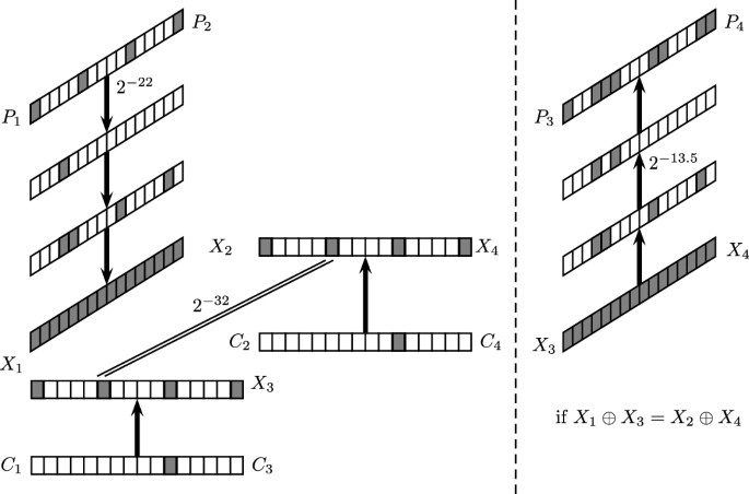
The attack on 5-round AES. In the attack of Biryukov [17] on 5-round AES, the cipher is decomposed as $E=E_1 \circ E_0$, where $E_0$ consists of the first 2.5 rounds and $E_1$ consists of the last 2.5 rounds. As usual, we denote the plaintexts involved in the boomerang attack by $P_1,P_2,P_3,P_4$, the corresponding ciphertexts by $C_1,C_2,C_3,C_4$, and the intermediate values at the input to $E_1$ by $X_1,X_2,X_3,X_4$. The attack is composed of the following components (see Fig. 7):

• For $E_0$ in the forward direction (i.e., for the pair $(P_1,P_2)$), the attack uses a truncated differential characteristic whose input difference can be any nonzero value in bytes 0, 5, 10, 15 and zero in all other bytes, and whose outputs have a zero difference in three shifted columns. (Note that the difference in the fourth column is not specified, as well as the position of the ‘active’ shifted column.) The probability of the characteristic is $2^{-22}$. Indeed, with probability $2^{-22}$, the difference after round 0 is nonzero in just one S-box, and then the truncated characteristic holds for sure.

• In $E_1$, the attack uses a truncated differential characteristic whose output difference can be any nonzero value in a single byte and zero in all other bytes. With probability 1, the corresponding difference in the input to round 3 is nonzero in only four bytes (that form an inverse shifted column). Hence, if two pairs $(C_1,C_3), (C_2,C_4)$ satisfy the output difference of the characteristic, then with probability $2^{-32}$, the four corresponding intermediate values at the input to round 3 sum up to zero. As MC is linear, this implies that $X_1 \oplus X_2 \oplus X_3 \oplus X_4 = 0$.

• In $E_0$ in the backward direction (i.e., for the pair $(X_3,X_4)$), the attack uses a different truncated differential characteristic. Note that if the characteristics of $E_0$ and $E_1$ described above are satisfied, then $X_3 \oplus X_4$ is nonzero in only a single shifted column. With probability of $6 \cdot 2^{-16} \approx 2^{-13.5}$, this leads to nonzero difference in only two bytes at the input of round 1. In such a case, $P_3$ and $P_4$ have zero difference in 8 bytes. (To be precise, there is zero difference in at least one of 6 possible sets of 8 bytes that form two inverse shifted columns.)

In total, starting with a plaintext pair $(P_1,P_2)$ and performing the boomerang process (with $\delta$ having a nonzero value in a single byte, which can be arbitrary), the resulting plaintexts $(P_3,P_4)$ have zero difference in one of six sets of 8 bytes with probability $2^{-22} \cdot 2^{-32} \cdot 2^{-13.5} = 2^{-67.5}$. In the attack, the adversary starts with structures of $2^{32}$ plaintexts that attain all possible values in bytes 0, 5, 10, 15 and are constant in the remaining bytes. For each structure, the adversary performs the boomerang process for all the plaintexts in the structure simultaneously and then uses a hash table to find all pairs $(P_1,P_2)$ in the structure for which the corresponding plaintexts $(P_3,P_4)$ have a zero difference in two inverse shifted columns. Each structure contains $2^{63}$ pairs that satisfy the input difference of the truncated characteristic for $E_0$, and hence, about $2^6$ structures (or $2^{38}$ plaintexts in total) are sufficient for containing a pair for which $(P_3,P_4)$ satisfies the property, with a very high probability. It should be mentioned that in addition to a right pair $(P_1,P_2)$ (i.e., a pair for which the boomerang property is satisfied), there are several more ‘random’ pairs that satisfy the condition, as the signal-to-noise ratio is less than 1. However, these pairs can be easily filtered out by auxiliary techniques.

Fig. 7

Biryukov’s 5-Round Boomerang Distinguisher for AES

Therefore, the attack allows distinguishing 5-round AES from a random permutation, with data and time complexity of $2^{39}$ and memory complexity of $2^{32}$.

Extension to 6-round AES. As was shown in [17], the 5-round attack described above can be easily extended into a distinguisher of 6-round AES with data and time complexity of $2^{71}$ and memory complexity of $2^{32}$. Indeed, denote the intermediate value before the last round in the encryption process of P by Y. The adversary guesses 4 subkey bytes in the last round. For each guess, she applies the 5-round attack, where for each pair $(P_1,P_2)$, the guessed subkey bytes allow finding the required change in the ciphertexts such that the obtained intermediate values $Y_3,Y_4$ will satisfy $Y_3 = Y_1 \oplus \delta$ and $Y_4 = Y_2 \oplus \delta$. The rest of the attack remains unchanged. Due to the extra subkey guess, the data and time complexities are increased from $2^{39}$ to $2^{71}$, while the memory complexity remains unchanged at $2^{32}$.

6.2 Improving the 5-Round Attack Using a Shifting Retracing Boomerang

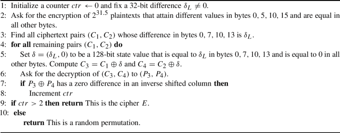
In the retracing boomerang attack, we use the decomposition $E=E_{12} \circ E_{11} \circ E_0$, where $E_0$ is the first 2.5 rounds like in Biryukov’s original attack, $E_{11}$ is the MC operation of round 2, and $E_{12}$ consists of rounds 3 and 4. Recall that we assume w.l.o.g. that the MC operation in round 4 is omitted, and thus, $E_{12}$ can be represented as four 32-bit to 32-bit super S-boxes applied in parallel (see [26]). Hence, we denote one of these super S-boxes by $E_{12}^L$ (w.l.o.g., in the sequel we take $E_{12}^L$ to be the super S-box whose output is bytes 0, 7, 10, 13) and concatenation of the other three by $E_{12}^R$. We fix $\delta _L$ to be some arbitrary output difference of $E_{12}^L$.

As in Biryukov’s attack, we encrypt a structure of M plaintexts that attain different values in bytes 0, 5, 10, 15 and are equal in all other bytes (where M will be determined below). Then, we filter the corresponding ciphertexts using a hash table, so that only pairs $(C_1,C_2)$ with difference $\delta _L$ in the output of $E_{12}^L$ remain.⁹ For each such pair, we ask for the decryption of $C_3 = C_1 \oplus \delta$, where $\delta =(\delta _L,0)$ (i.e., difference $\delta _L$ in $E_{12}^L$ and difference 0 in $E_{12}^R$) and $C_4 = C_2 \oplus \delta$, and check a condition (explained shortly) on the corresponding plaintexts $(P_3,P_4)$.

Note that for each examined quartet $((C_1,C_2),(C_3,C_4))$, the four corresponding inputs to $E_{12}^L$ are composed of two pairs of equal values and thus sum up to zero, and so are the four corresponding inputs to $E_{12}^R$. As $E_{11}$ is linear (consisting of a single MC operation), this implies that the four inputs of $E_{11}$, namely $X_1,X_2,X_3,X_4$, sum up to zero with probability 1! Thus, with probability of $2^{-22}$, the difference $X_3 \oplus X_4$ equals zero in all bytes except for a shifted column. This lies in sharp contrast with the original boomerang attack, where the same event holds with probability $2^{-54}$.

We can use the increased probability to replace the truncated differential characteristic used for $(E_{0})^{-1}$ by a characteristic with a higher probability that predicts the difference in a smaller part of the state. (Here, we use the improved signal-to-noise ratio in the retracing boomerang attack.) Specifically, if $X_3 \oplus X_4$ is nonzero in only a single shifted column, then with probability of $4 \cdot 2^{-8} = 2^{-6}$, this leads to nonzero difference in only three bytes at the input of round 1. In such a case, $P_3$ and $P_4$ have a zero difference in 4 bytes. (To be precise, there is zero difference in at least one of 4 possible sets of 4 bytes that form an inverse shifted column.) Note that for a random permutation, this property holds with probability $2^{-30}$, instead of the much lower probability of $2^{-61.5}$ of the property used in Biryukov’s attack. However, for the cipher E, the property holds with probability $2^{-22} \cdot 2^{-6}=2^{-28}$, and hence, this weaker filtering is sufficient for leaving only a few wrong pairs.

Algorithm 5

Our Enhancement of Biryukov’s Boomerang Attack on 5-Round AES

Our resulting attack algorithm is presented in Algorithm 5.

Analysis of the attack. The structure of plaintexts contains $2^{62}$ plaintext pairs. About $2^{62} \cdot 2^{-32} = 2^{30}$ of them are expected to satisfy the condition on $C_1 \oplus C_2$, and hence, the decryption process is performed for $2^{30}$ pairs. For a random permutation, as the probability of the condition on $P_3 \oplus P_4$ is $2^{-30}$, then the expectation of the final value of count is 1. On the other hand, for E, out of the $2^{30}$ examined pairs, $2^{30} \cdot 2^{-22} = 2^8$ are expected to satisfy the characteristic in $E_0$ and out of them, $2^8 \cdot 2^{-6} = 4$ are expected to satisfy the characteristic in $(E_0)^{-1}$. Therefore, the expectation of the final value of count is 4, and so, the attack indeed distinguishes E from a random permutation with a very high probability.

It is clear that the attack complexity is dominated by encrypting and storing the data, and hence, its data, memory, and time complexities are $2^{31.5}$. We note that the complexity of the attack can be reduced a bit further, using a fine tuning of the characteristics used in the attack.

Related work. A distinguisher with a lower complexity of $2^{25.8}$ on 5-round AES with a secret S-box was obtained by Rønjom et al. [46]. Our distinguisher has a somewhat higher complexity, but is more general, as the distinguisher of [46] uses the MDS property of the MC matrix (see [44]), while our distinguisher does not make any assumptions on the S-box or on the MC matrix. We note, however, that our key recovery attack on 5-round AES with a secret S-box, presented in Sect. 5, can be used to distinguish 5-round AES in time $2^{29}$, which is somewhat faster than the attack presented here, without any assumption on the MC operation.

6.3 Improving the 6-Round Attack Using a Shifting Retracing Boomerang

Attack description. At first glance, it seems that there is no way to add a round to the retracing boomerang attack presented above, since in order to recover the outputs of $E_{12}^L$, one has to guess the entire final subkey. However, an extension turns out to be possible. The basic observation we use here is that the 5-round attack presented above works for any choice of $\delta$. In particular, we may take $\delta$ that has a nonzero value in a single byte. Then, it is sufficient to guess 4 bytes of the last round key in order to be able to modify the ciphertexts in such a way that the obtained intermediate values $Y_3,Y_4$ satisfy $Y_3 = Y_1 \oplus \delta$ and $Y_4 = Y_2 \oplus \delta$. (Note that only the nonzero byte of $\delta$ is taken care of by our modification. The zero bytes of $\delta$ hold automatically, since we do not change the ciphertexts at all in the three shifted columns that affect them.)

At this point, it seems that there is an additional obstacle. Due to the added round at the end, we cannot perform the filtering in the middle of the attack, since we do not know whether the intermediate values $Y_1,Y_2$ have difference 0 or $\delta$ in the output of $E_{12}^L$ or not. (Actually, we can check this in one out of the four bytes, due to the key guess, but not in the other bytes.) To overcome this issue, we continue the attack with all pairs and filter out the wrong ones at a later stage. This increases the data and time complexities, but we can reduce this ‘penalty’ by performing the modification and decryption for the entire plaintext structure at once, and checking specific pairs only at a later stage.

In order to reduce the data complexity of the attack, we use a method that was presented in [46] and is used also in our attack on 5-round AES in Sect. 4. We replace the truncated differential characteristic used for $(E_0)^{-1}$ by a characteristic with a higher probability that predicts the difference not between the plaintexts $(P_3,P_4)$, but rather between intermediate values after one round of encryption. Specifically, let Z denote the intermediate value after round 0 in the encryption process of P. For $E_0$ in the forward direction, we use a truncated differential characteristic whose output difference is zero in a single shifted column. The probability of the characteristic is $4 \cdot 2^{-8}=2^{-6}$. For the backward direction, note that if $X_3 \oplus X_4$ has a zero difference in a shifted column, then with probability 1, the corresponding difference $Z_3 \oplus Z_4$ equals zero in an inverse shifted column. Furthermore, the same property holds for any pair $(Z'_3,Z'_4)$ obtained by shifting the values $(Y_1,Y_2)$ by some other value $\delta '$ instead of $\delta$. Hence, we can collect several such ‘friend pairs’ (see Sect. 8) and use the zero difference in an inverse shifted column between $Z_3$ and $Z_4$ in all these pairs to attack the subkey of round 0.

The algorithm of our attack is given in Algorithm 6.

Algorithm 6

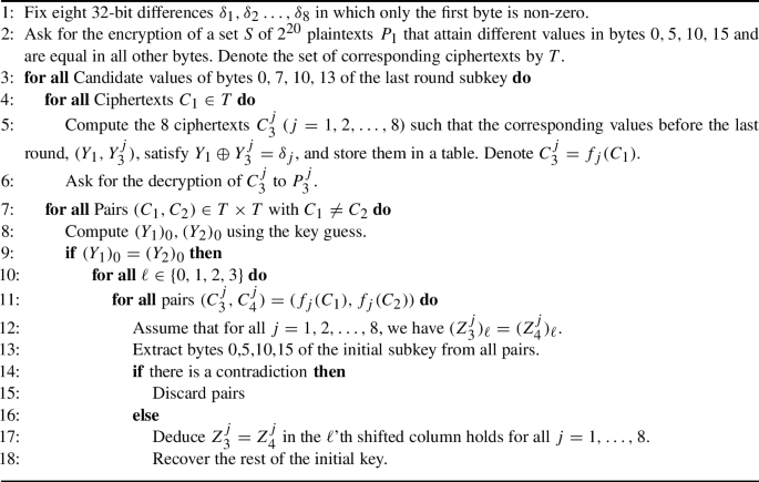
Shifting Retracing Boomerang Attack on 6-Round AES

Attack analysis. The $2^{20}$ chosen plaintexts contain $2^{39}$ pairs. Out of them, $2^{39} \cdot 2^{-6} \cdot 2^{-32} = 2$ are expected to satisfy both the truncated differential characteristic in $E_0$ and the condition on $Y_1 \oplus Y_2$. For each such pair, and for each j, all eight pairs $(Z^j_3,Z^j_4)$ must satisfy $(Z^j_3)_{\ell } = (Z^j_4)_{\ell }$ for some $\ell \in \{0,1,2,3\}$, and thus, once such a pair is encountered, the attack recovers bytes 0,5,10,15 of the key, and consequently, the entire key. For a wrong pair, as the attack on bytes 0,5,10,15 contains a 64-bit filtering, the probability that there is no contradiction is only $2^{-32}$, and thus, only a few wrong pairs survive these step. Those pairs are filtered in the attacks on the rest of the initial subkey, as each such attack provides an additional 32-bit filtering. Therefore, our algorithm recovers the entire secret key with a high probability.

The data complexity of our attack is $2^{20} \cdot 8 \cdot 2^{32} = 2^{55}$ ACCs. The time complexity is dominated by the procedure of finding bytes 0,5,10,15 of the initial key. This procedure is performed for $2^{39} \cdot 2^{-8}=2^{31}$ pairs, for each of $2^{32}$ guesses of the last round subkey, and each of 4 values of $\ell$. Since it can be performed in a meet-in-the-middle fashion, each application requires about $2^{16}$ 2-round encryptions, which are less than $2^{15}$ 6-round encryptions. Hence, the overall time complexity is less than $2^{31} \cdot 2^{32} \cdot 4 \cdot 2^{15} = 2^{80}$ encryptions. The memory complexity is $2^{31}$, dominated by storing the pairs examined in the attack on the initial subkey.

Related work. A boomerang attack with a lower time complexity of $2^{61}$ on 6-round AES was obtained by Bariant and Leurent [7]. Our attack has a higher time complexity, but lower data and memory complexities ($D=2^{55}$ vs. $D=2^{59}$ in [7], and $M=2^{31}$ vs. $M=2^{59}$ in [7]). It will be interesting to find out whether our technique can be combined with the technique of [7] to obtain an attack which simultaneously improves the data, the memory, and the time complexity.

Two remarks. We conclude this section with two remarks. First, the main interest in this 6-round attack is demonstration of the abilities of the new retracing boomerang technique. Its actual result is not very interesting, as there exist significantly stronger attacks on 6-round AES—most notably, the Square attack [31] with data complexity of $2^{34}$ chosen plaintexts and time complexity of $2^{42}$ encryptions.

Second, we note that unlike the 5-round attack where the mixing type of the retracing boomerang can be applied instead of the shifting variant we used, with roughly the same complexity, in this case the mixing variant cannot be used at all. Indeed, in order to perform mixing, we have to know the entire outputs of $E_{12}^L$, and this necessitates guessing the entire last round subkey. The shifting retracing boomerang allows us to perform the modification of the ciphertexts while being in control of only a single byte in the output of $E_{12}^L$. This demonstrates one of the advantages of the shifting retracing boomerang attack over the mixing variant.

7 The Retracing Rectangle Attack—Connection to Mixture Differentials

In this section, we present the retracing rectangle attack, which is the retracing variant of the rectangle attack [11, 37]. First we recall the amplified boomerang (a.k.a. rectangle) attack, then we present and analyze the new retracing rectangle attack, and then, we use our new framework to expose a relation of the recently introduced mixture differential attack [33] to the rectangle attack.

7.1 The Amplified Boomerang (a.k.a. Rectangle) Attack

An apparent drawback of the boomerang attack is the need to use adaptively chosen plaintexts and ciphertexts—a very strong ability for the attacker. In [37], Kelsey et al. presented the amplified boomerang attack, which imitates the procedure of the boomerang attack using only chosen plaintexts. In the attack, the adversary considers pairs of pairs of plaintexts $((P_1,P_2),(P_3,P_4))$ such that $P_1 \oplus P_2 = P_3 \oplus P_4 = \alpha$, and for each of them, she checks whether the corresponding quartet of ciphertexts $((C_1,C_2),(C_3,C_4))$ satisfies $C_1 \oplus C_3 = C_2 \oplus C_4 = \delta$.

The analysis of the attack is as follows. By the differential characteristic of $E_0$, with probability $p^2$ we have $X_1 \oplus X_2 = X_3 \oplus X_4 = \beta$, and thus, $X_1 \oplus X_3 = X_2 \oplus X_4$. Assuming that these differences are equal to $\gamma$, which happens with probability $2^{-n}$ under standard randomness assumptions, the differential characteristic of $E_1$ implies that $C_1 \oplus C_3 = C_2 \oplus C_4 = \delta$ holds with probability $q^2$. Hence, we expect that the two equalities $C_1 \oplus C_3 = C_2 \oplus C_4 = \delta$ hold for a fraction of $p^2 q^2 2^{-n}$ of the quartets. Since for a random permutation, these two equalities hold with probability $2^{-2n}$, the attack can distinguish E from a random permutation if $pq \gg 2^{-n/2}$. The data complexity of the attack is $4 \cdot 2^{n/2} (pq)^{-1}$, as this is the amount of plaintexts required for constructing $2^n (pq)^{-2}$ quartets. While it may seem that the time complexity is as high as $O(2^n (pq)^{-2})$ (which is the number of quartets we have to check), it can be actually reduced to $O(2^{n/2} (pq)^{-1})$, by using hash tables.

Kelsey et al. applied the amplified boomerang attack to the AES’ candidates MARS and Serpent. In a subsequent work, Biham et al. [11] presented several enhancements of the attack (in particular, allowing to use many differentials in parallel, like Wagner’s suggestion for the original boomerang attack, see ‘Appendix A’), and gave it the name rectangle attack, which is the currently more commonly-used name.

7.2 The Retracing Rectangle Attack

The transformation from the retracing boomerang attack to the retracing rectangle attack is similar to the transformation from the (classical) boomerang attack to the rectangle attack.

The attack setting. We assume that E can be decomposed as $E = E_1 \circ E_{02} \circ E_{01}$, where $E_{01}$ consists of dividing the state into two parts (a left part of b bits and a right part of $n-b$ bits) and applying to them the functions $E_{01}^L,E_{01}^R$. Furthermore, we suppose that for $E_{01}^L$, there exists a differential characteristic $\alpha _L \xrightarrow {p_1^L} \mu _L$, for $E_{01}^R$, there exists a differential characteristic $\alpha _R \xrightarrow {p_1^R} \mu _R$, for $E_{02}$, there exists a differential characteristic $\mu \xrightarrow {p_2} \beta$, and for $E_{1}$, there exists a differential characteristic $\gamma \xrightarrow {q} \delta$ (see Fig. 8).

Fig. 8

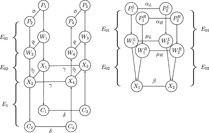
The Retracing Rectangle Setting

Assuming that $pq_1 q_2^L q_2^R \gg 2^{-n/2}$, the rectangle attack can be used to distinguish E from a random permutation, with data complexity of $O((pq_1 q_2^L q_2^R)^{-1} \cdot 2^{n/2})$ chosen plaintexts. Recall that in the standard rectangle attack, we consider quartets of plaintexts $((P_1,P_2),(P_3,P_4))$ such that $P_1 \oplus P_2=P_3 \oplus P_4=\alpha$, and check whether the corresponding quartets of ciphertexts $((C_1,C_2),(C_3,C_4))$ satisfy $C_1 \oplus C_3 = C_2 \oplus C_4 = \delta$. In the retracing rectangle attack, we consider only quartets of plaintexts that satisfy

$$\begin{aligned} (P_1 \oplus P_2=\alpha ) \wedge (P_3 \oplus P_4 =\alpha ) \wedge ((P_1)^L \oplus (P_3)^L = 0 \text{ or } \alpha ^L). \end{aligned}$$

(14)

As a result, the two unordered pairs $(P_1^L,P_2^L)$ and $(P_3^L,P_4^L)$ are identical, and hence, if one of them satisfies the differential characteristic of $E_{01}^L$, then so does the other. Thus, the probability of the rectangle distinguisher is improved by a factor of $(p_1^L)^{-1}$.

Advantages. Unlike the shifting retracing boomerang attack, here we obtain an improvement in the probability of the distinguisher without a need to discard some part of the data. (This holds since the adversary can choose the plaintexts as she wishes, and in particular, can force the additional restriction $(P_1^L \oplus P_3^L = 0 \text{ or } \alpha ^L)$ ‘for free.’) In addition, the signal-to-noise ratio is improved, like in the retracing boomerang attack, which can result in a reduced data complexity.

It should, however, be noted that in most applications of the rectangle attack, the adversary starts with structures S of pairs with input difference $\alpha$, such that each pair-of-pairs within the same structure satisfies the initial condition of the rectangle distinguisher. Then, for each structure, the adversary uses a hash table to check all these ${{|S|}\atopwithdelims (){2}}$ quartets in time |S|. In the retracing rectangle attack, one has to either give up the structures and work with each pair-of-pairs that satisfies Eq. (14) separately, or else perform the ordinary rectangle attack and then check the additional condition $(P_1^L \oplus P_3^L = 0 \text{ or } \alpha ^L)$ simultaneously with the condition $C_1 \oplus C_3 = C_2 \oplus C_4 = \delta$ (which can be done using a hash table). In both cases, the overall data complexity of the attack is not reduced, compared to the rectangle attack with structures, and thus, improvement of the signal-to-noise ratio is the main advantage of the retracing rectangle technique.

A mixing variant—relation to mixture differentials. Like in the mixing retracing boomerang attack, the adversary can force equality between the unordered pairs $(P_1^L,P_2^L),(P_3^L,P_4^L)$ by choosing $P_3 = (P_2^L,P_1^R)$ and $P_4 = (P_1^L,P_2^R)$, or in other words, by taking the pair $(P_3,P_4)$ to be the mixture counterpart of the pair $(P_1,P_2)$. As this choice also forces equality between the pairs $(P_1^R,P_2^R)$ and $(P_3^R,P_4^R)$, the probability of the rectangle distinguisher is increased by a factor of $(p_1^L p_1^R)^{-1} = p_1^{-1}$.

Interestingly, it turns out that the core step of the mixture differential attack of Grassi [33] on 5-round AES fits into the mixture retracing rectangle attack framework. Specifically, the core of [33]’s result is a chosen plaintext distinguishing attack on a 3.5-round variant of AES. In this attack, 3.5-round AES is decomposed as $E_1 \circ E_{02} \circ E_{01}$, where $E_{01}$ consists of the first 1.5 rounds, $E_{02}$ consists of a single MC layer, and $E_1$ is composed of the last 1.5 rounds. The attack uses quartets of plaintexts $(P_1,P_2,P_3,P_4)$ constructed by a mixing procedure, as described in Definition 1, and considers the corresponding quartets $(X_1,X_2,X_3,X_4)$ and $(Y_1,Y_2,Y_3,Y_4)$ of intermediate values after $E_{01}$ and $E_{02}$, respectively. The representation of 1.5-round AES as four Super-S-boxes applied in parallel [26] allows deducing that $X_1 \oplus X_2 \oplus X_3 \oplus X_4=0$ holds with probability 1. As $E_{02}$ is linear, the same holds for $Y_1,Y_2,Y_3,Y_4$. Finally, the attack uses a truncated differential characteristic of $E_1$ with probability 1 that starts with difference 0 in an inverse shifted column (e.g., bytes 0, 5, 10, 15) and ends with difference 0 in a shifted column (e.g., bytes 0, 7, 10, 13). (This characteristic also follows from the Super-S-boxes representation of 1.5-round AES.) If the pair $(Y_1,Y_3)$ satisfies the input difference of this characteristic – an event that occurs with probability of $2^{-32}$—then $(Y_2,Y_4)$ satisfies the input difference as well, and then, we know for sure that both $(C_1,C_3)$ and $(C_2,C_4)$ have zero difference in bytes 0, 7, 10, 13. This provides a 64-bit filtering that is exploited in [33] to obtain a key recovery attack on 5-round AES.

While this may not be apparent at a first glance, this attack is indeed a variant of the mixing retracing rectangle attack described above. The choice of plaintext quartets is exactly the same, and so is the treatment of $E_1$ (taking note that the differential characteristics used in a boomerang/rectangle attack may be truncated, as mentioned above). The only seeming difference is $E_0$, where instead of considering a specific differential characteristic we only make sure that the four outputs sum up to zero. However, this is actually the same as using all possible differential characteristics simultaneously, as is commonly done in boomerang/rectangle attacks (see ‘Appendix A’).

8 Different Methods of Generating ‘Friend Pairs’

An important ingredient in many cryptanalytic attacks is friend values, i.e., values that are attached to given values in such a way that if a given value satisfies some desired property, then all its friend values satisfy the same property as well. Friend values amplify the advantage obtained by satisfying the property, and are frequently used to discard wrong suggestions. (See, e.g., [3] and [8] for the central role of friend values in slide attacks and in differential-linear attacks, respectively.)

In the boomerang attack, the friend values are actually friend pairs attached to given pairs, in such a way that if a pair satisfies some of the differential characteristics underlying the boomerang distinguisher, then so do all its friend pairs.

Friend pairs play a central role in all attacks presented in this paper, and hence, a discussion on the possible ways to generate friend pairs is due. In this paper, we use (or mention) three different ways of generating friend pairs:

• Attaching plaintext pairs $(P^j_1,P^j_2)$ to each pair $(P_1,P_2)$, in such a way that if $(P_1,P_2)$ satisfies the differential characteristic for $E_0$, then so do all its friend pairs. This strategy is possible if there exist plaintext bits that do not affect the output difference of $E_0$, given that the input difference is fixed to $\alpha$ (i.e., the input difference of the differential characteristic used in $E_0$). For example, this is the case in all our attacks on 5-round AES. The advantage in this approach is that it can be combined with the use of structures. Indeed, given a structure S, one can construct ‘friend structures’ by XORing the same (properly chosen) value to all plaintexts in the structure, thus providing all pairs in the structure with friend pairs simultaneously.

• Attaching ciphertext pairs $(C^j_3,C^j_4)$ to each ciphertext pair $(C_1,C_2)$. This strategy is possible if there exist many differential characteristics of the form $\gamma \xrightarrow {q_j} \delta _j$ for $E_1$. In the shifting retracing attack, this strategy can be combined with the use of structures, as the entire structure can be shifted by several values of $\delta$ instead of a single value. Furthermore, in such cases this strategy can be used to construct a large amount of friend pairs, since each characteristic $\gamma \xrightarrow {q_j} \delta _j$ gives rise to a different friend pair. In the mixing retracing attack, structures cannot be used as one has to work with each pair separately, and only a few friend pairs can be generated. For example, in the case of AES, up to $2^{32}$ friend pairs for each pair can be generated in the shifting retracing attack, while only 7 friend pairs can be generated for each pair in the mixing retracing attack (see [33]). This is yet another advantage of the shifting retracing technique over the mixing retracing technique, as we mentioned in Sect. 3.2.

• The yoyo process—encrypting a pair of plaintexts, modifying the resulting ciphertexts and decrypting them, modifying the resulting plaintexts and encrypting them, etc. (see [46]). While this is arguably the most interesting among the three ways of generating friend pairs we discussed, this strategy has the disadvantage of requiring a multi-round sequence of adaptively chosen plaintext/ciphertext queries, which renders such an attack unrealistic in most scenarios. Hence, in our attacks we use only the first two ways of generating friend pairs, and not the third one.

Finding more ways to generate friend pairs will be very interesting.

9 Summary and Open Problems

In this paper, we introduced a new version of boomerang attacks called a retracing boomerang attack and used it to significantly improve the best known key recovery attacks on 5 rounds of AES. (Both in its standard form and when the S-box and the linear transformation are secret key-dependent components.) The most interesting problems left open in this paper are:

• Find additional applications of the new technique.

• Find other types of correlations which can further increase the probability of the combined differential property.

• Create a ‘grand unified theory’ of boomerang-like attacks which will explore their hidden relationships and treat them rigorously.

Variants and Extensions of the Boomerang attack

In this appendix, we present several variants/extensions of the boomerang attack that are related to our new retracing boomerang attack. After briefly presenting each variant, we explain its relation to our work.

1.1 Using Truncated Differentials in the Boomerang Attack

A truncated differential characteristic is a characteristic that predicts the difference in only part of the state. Truncated differential characteristics were mentioned already in [16] and were fully developed by Knudsen [40]. In [50], Wagner observed that the boomerang attack can exploit truncated differential characteristics, if several difficulties are addressed. First, in the truncated setting, the equivalence between the differential characteristic $\gamma \xrightarrow {q} \delta$ for $E_1$ and the differential characteristic $\delta \xrightarrow {q} \gamma$ for $E_1^{-1}$ does not hold anymore. Moreover, Eq. (3) no longer holds for sure, if the values $\beta ,\gamma$ correspond to only part of the intermediate state bits. Finally, if the characteristic used for the pair $(X_3,X_4)$ in the backward direction does not predict the full difference $P_3 \oplus P_4$, then the probability that the property holds for a random permutation is higher than $2^{-n}$. Nevertheless, Wagner showed that the analysis can be adapted to this case as well (of course, at the expense of increasing the data complexity of the attack). This extension was used in various cases, in particular by replacing the differential characteristic used for the pair $(X_3,X_4)$ in the backward direction with a truncated characteristic in order to increase the overall probability, in cases where pq was much higher than $2^{-n/2}$ (see, e.g., [7] and [17]).

Relation to the retracing boomerang attack. Truncated differential characteristics play a central role in our attacks. In fact, all characteristics we use in this paper are truncated.

1.2 Adding a Round to the Boomerang Distinguisher Using Structures

A common technique for extending the applicability of the boomerang attack is appending a round before or after the boomerang distinguisher (see, e.g., [12]).

Adding a round at the beginning. Assume that E can be decomposed as $E_1 \circ E_0 \circ E'$, where for $E_1 \circ E_0$ there exists a boomerang distinguisher with probability $(pq)^2$ that starts (and ends) at difference $\alpha$. Let $\chi ,\chi '$ be intermediate values after the application of $E'$ such that $\chi \oplus \chi ' = \alpha$, and consider the corresponding plaintexts $P=(E')^{-1}(\chi )$ and $P'=(E')^{-1}(\chi ')$. Of course, the difference $P \oplus P'$ is not fully determined by the assumption $\chi \oplus \chi ' = \alpha$ (unless $E'$ is linear), but in many cases, P and $P'$ must be equal in a large part of the state. Let us decompose the plaintext P as $P=(P_{passive},P_{active})$, where the difference in the part $P_{passive}$ is known with probability 1. We denote by $\ell$ the number of bits in $P_{active}$. These notations are given in Fig. 9.

Fig. 9

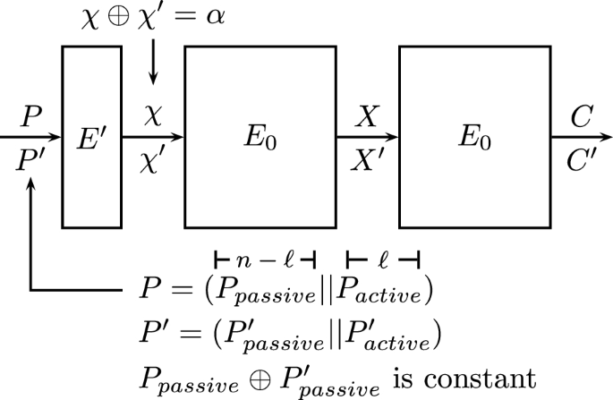
Attacking Rounds Before the Boomerang Distinguisher

In the following description of the distinguisher, we assume that the difference $P_{passive} \oplus P'_{passive}$ is fixed to zero. The transformation of the described procedure to the case of $P_{passive} \oplus P'_{passive} = \textrm{const} \ne 0$ is immediate and does not change the complexities. One can mount a distinguisher for E as follows. Consider structures S of $2^{\ell }$ plaintexts each, such that in each structure, the bits of $P_{passive}$ are equal for all the values in the structure and the bits of $P_{active}$ attain all $2^{\ell }$ possible values. For each structure, encrypt the entire structure S to obtain $2^{\ell }$ ciphertexts, then modify each of them by XORing $\delta$ to it, and decrypt the $2^{\ell }$ resulting ciphertexts to obtain a structure $S'$ of plaintexts. Find all pairs in $S'$ that have zero difference in the bits of $P_{passive}$.

Note that each structure contains $2^{2\ell -1}$ pairs $(P_1,P_2)$, and for $2^{\ell -1}$ of them, the corresponding intermediate difference $\chi _1 \oplus \chi _2$ equals $\alpha$. For a fraction of $(pq)^2$ of those $2^{\ell -1}$ pairs, the corresponding intermediate values ‘on the way back of the boomerang’ satisfy $\chi _3 \oplus \chi _4 = \alpha$, and thus, the corresponding plaintexts $P_3,P_4$ have zero difference in the bits of $P_{passive}$. Thus, if we take $(pq)^{-2} / 2^{\ell -1}$ structures, then with probability of about $1-1/e$, we are expected to find at least one pair $(P_3,P_4)$ which is a part of a right quartet, i.e., with zero difference in the bits of $P_{passive}$. If p, q are sufficiently large, then this probability is larger than the corresponding probability for a random permutation, and hence, the distinguisher succeeds. Otherwise, one can perform analysis of the key used in $E'$, using the fact that right quartets will always suggest the correct value of the key used in $E'$.

The data complexity of the distinguisher is $((pq)^{-2} / 2^{\ell -1}) \cdot 2^{\ell }\cdot 2 = 4(pq)^{-2}$ ACCs, which is exactly the same as in the boomerang distinguisher for $E_1 \circ E_0$. Therefore, we extended the distinguisher to include also $E'$, without increasing the data complexity.

Adding a round at the end. In a similar way, one can add a round at the end of the distinguisher. This time, E is decomposed as $E = E'' \circ E_1 \circ E_0$ and it is assumed that there exists a boomerang distinguisher for $E_1 \circ E_0$ whose output difference is $\delta$. We consider pairs of intermediate values $\chi ,\chi '$ before $E''$, assume that $\chi \oplus \chi '=\delta$, and check the difference between $C=E''(\chi )$ and $C'=E''(\chi ')$. If the ciphertexts can be divided into two parts: $C_{passive}$ (of size $n-\ell$ bits) in which the difference is known when $\chi \oplus \chi ' =\delta$, and the remaining $\ell$ bits $C_{active}$ whose difference is unknown, then we can extend the boomerang distinguisher to contain also $E''$ in the following way. (Similarly to the extension by $E'$ presented above, we assume that $C_{passive} \oplus C'_{passive}=0$; the modification required for dealing with another constant instead of 0 is straightforward.)

We start with pairs $(P_1,P_2)$ with difference $\alpha$ and encrypt them through E. For each ciphertext pair $(C_1,C_2)$, we consider the $2^{\ell }$ possible values $C^j_3$ of the form $C_1 \oplus \eta _j$, where $\eta _j$ is equal to zero in the bits of $C_{passive}$, and similarly, the $2^{\ell }$ possible values $C^j_4$ of the form $C_2 \oplus \eta _j$. We decrypt these values and obtain two pools of $2^{\ell }$ plaintexts $\{P^j_3\}$ and $\{P^j_4\}$. Using a hash table, we find all pairs $j,j'$ such that $P^j_3 \oplus P^j_4 = \alpha$.

An analysis similar to the analysis presented above shows that if p, q are sufficiently large, then this variant allows to insert $E''$ into the distinguisher. However, unlike the case of adding a round at the top, here the data and time complexities of the attack are increased by a factor of $2^{\ell }$, as for each encrypted plaintext, we have to decrypt $2^{\ell }$ modified ciphertexts. Note that in this variant of the attack, the number of decrypted ciphertexts is significantly larger than the number of encrypted plaintexts.

Adding rounds on both sides. Finally, in some cases both extensions can be combined into an attack that extends the basic boomerang distinguisher by two rounds—one round on each side. We omit the details and refer the interested reader to [12].

Relation to the retracing boomerang attack. Extension of the boomerang distinguisher by one round at the end is one of the cases where shifting retracing boomerang is advantageous over the standard boomerang attack. The reason for the advantage is that in this case, the number of decryptions in the attack is much larger than the number of encryptions, and hence, the reduction in the number of decryptions obtained in the shifting retracing boomerang framework reduces the overall data complexity of the attack significantly. In addition, structures play a central role in all our attacks.

1.3 Using Several Differential Characteristics in Parallel in the Boomerang Attack

In [50], Wagner observed that the probability of the boomerang distinguisher can be increased by using many differential characteristics in parallel. Assume that in addition to the differential characteristic $\alpha \xrightarrow {p} \beta$, there exists another characteristic $\alpha \xrightarrow {p'} \beta '$. Then by the same analysis as in the basic boomerang attack, for each pair $(P_1,P_2)$ that satisfies the alternative characteristic, if the corresponding ciphertexts satisfy Eq. (2), then we have $X_3 \oplus X_4 = \beta '$, and thus, $P_3 \oplus P_4 = \alpha$ holds with probability $p'$. The pairs counted here are disjoint from the pairs counted for the characteristic $\alpha \xrightarrow {p} \beta$, and hence, overall we have

$$\begin{aligned} \Pr [P_3 \oplus P_4 = \alpha | P_1 \oplus P_2 = \alpha ] \ge (p^2 + (p')^2) q^2. \end{aligned}$$

The same holds for the differential characteristics of $E_1$. Hence, the overall lower bound on the probability of the boomerang distinguisher can be enhanced to

$$\begin{aligned} \sum _{\beta ',\gamma '} \Pr [\alpha \xrightarrow [E_0]{~} \beta ']^2 \Pr [\gamma ' \xrightarrow [E_1]{~} \delta ]^2 = (\hat{p} \hat{q})^2, \end{aligned}$$

(15)

where $\Pr [\alpha \xrightarrow [{E_0}]{~} \beta ']$ is the probability of the differential characteristic $\alpha \rightarrow \beta '$ through $E_0$ and $\hat{p}$ is defined as $\hat{p}=\sqrt{\sum _{\beta '} \Pr [\alpha \xrightarrow [{E_0}]{~} \beta ']^2}$, and similarly for $\hat{q}$. In many cases, this ability to take into account multiple differential characteristics significantly improves the boomerang attack.

Relation to the retracing boomerang attack. For sake of simplicity, throughout the paper we considered the case where only a single characteristic is available for each sub-cipher. The retracing boomerang attack readily combines with the use of several characteristics in parallel; for example, in the shifting retracing boomerang attack, the probability p can be upgraded to $\hat{p}$ and the probability q can be upgraded to $\hat{q}$. A specific example of using multiple differential characteristics in the retracing framework is the mixture differential attack on 5-round AES, discussed (and presented inside the retracing rectangle framework) in Sect. 7.

1.4 Related-key Boomerang and Rectangle Attacks

In 2004, Kim et al. [39], and independently, Biham et al. [13], observed that the boomerang attack can be used also in the related-key setting [9], where the attacker can request for encryption under several (unknown) keys with a known (or even chosen) relation between them, and her goal is to recover the keys. In order to briefly present this attack, we need an additional notation. We say that the related-key differential characteristic $\varOmega _I \xrightarrow [{E,\varDelta K}]{~} \varOmega _O$ holds with probability p if

$$\begin{aligned} \Pr [E_K(P) \oplus E_{K \oplus \varDelta K}(P \oplus \varOmega _I) = \varOmega _O] = p, \end{aligned}$$

where $E_K(P)$ denotes encryption of P with the cipher E, using the secret key K. In the related-key boomerang attack, we assume that there exist related-key differentials $\alpha \xrightarrow [E_0,\varDelta K_{ab}]{~} \beta$ for $E_0$ with probability p and $\gamma \xrightarrow [{E_1,\varDelta K_{ac}}]{~} \delta$ for $E_1$ with probability q. In the attack, the adversary considers pairs of plaintexts $(P_1,P_2)$ with difference $\alpha$, and for each of them, she asks for the encryption of $P_1$ under the secret key $K_a$ and for the encryption of $P_2$ under the related-key $K_b = K_a \oplus \varDelta K_{ab}$. Then, she modifies the corresponding ciphertexts $C_1,C_2$ into $C_3 = C_1 \oplus \delta , C_4 = C_2 \oplus \delta$, and asks for the decryption of $C_3,C_4$ under the related-keys $K_c = K_a \oplus \varDelta K_{ac}$ and $K_d = K_b \oplus \varDelta K_{ac}$. She then checks whether the corresponding plaintexts $P_3,P_4$ satisfy $P_3 \oplus P_4 = \alpha$.

An analysis similar to that of the basic boomerang attack shows that for the cipher E, the equation $P_3 \oplus P_4 = \alpha$ holds with probability $(pq)^2$. A key observation used here is that

$$\begin{aligned} K_c \oplus K_d= & {} (K_c \oplus K_a) \oplus (K_a \oplus K_b) \oplus (K_b \oplus K_d) \\= & {} \varDelta K_{ac} \oplus \varDelta K_{ab} \oplus \varDelta K_{ac} = \varDelta K_{ab}, \end{aligned}$$

and thus, the related-key differential of $E_0$ can be applied to the decryption of the pair $(X_3,X_4)$ through $E_0$.

Like in the basic boomerang attack, one can use many related-key differentials in parallel, utilize related-key truncated differentials, and transform the attack into a chosen plaintext attack. The related-key boomerang attack proved to be especially strong and was used to mount the only known attack on the full AES which is significantly faster than exhaustive search (on the 192-bit and 256-bit key variants) [19], a practical-time attack on KASUMI—the cipher of 3 G cellular networks [30], and many other attacks.

Relation to the retracing boomerang attack. Retracing boomerang can be readily combined with related-key differentials, provided that there is no key difference that affects the values whose equality we force (e.g., the key difference $\varDelta K_{ac}$ equals zero in the bits that affect $E_{12}^L$) or that a key difference in those values is cancelled out with a carefully chosen data difference.

1.5 Rigorous Analysis of the Probability of the Boomerang Distinguisher

While the S-box switch presented in Sect. 2.2 demonstrates how dependency between the differentials can be used in favor of the adversary, Murphy [42] showed that in various cases of interest, such dependency may increase the complexity of the boomerang attack and even reduce its success probability significantly. Many additional examples show that the naive assumption of independence between differential characteristics fails badly (in both directions) in various realistic scenarios (e.g., [18, 19, 30, 38]).

In [30], Dunkelman et al. proposed the sandwich framework in order to take into account the dependency between the sub-ciphers in the attack analysis. Recently, Cid et al. [24] proposed the boomerang connectivity table (BCT), which allows computing the complexity of the boomerang attack more accurately and, moreover, enables the adversary to choose the differential characteristics of $E_0$ and $E_1$ in a way that exploits the dependency between the sub-ciphers to amplify the overall probability of the boomerang distinguisher. Several follow-up papers studied and extended the BCT (e.g., [22, 23, 51]), and this area is far from being fully explored.

Relation to the retracing boomerang attack. In this paper, we presented the basic idea of the retracing boomerang attack and relied on simplistic randomness assumptions, without going into rigorous probability computations. The next logical step, which we leave for further research, is to develop a framework (e.g., similar to the sandwich framework or to the BCT, which currently address only dependency between the two sub-ciphers and not dependency inside the same sub-cipher) that will allow for a rigorous probability computation also for the retracing boomerang attack.

References

X. An, H. Kai, W. Meiqin. Mixcolumns coefficient property and security of the AES with a secret s-box, in Proceedings of AFRICACRYPT 2020, volume 12174 of LNCS (Springer, 2020), pp. 114–131
V. Arlazarov, E. Dinic, A. M. Kronrod, I. Faradžev, On economical construction of the transitive closure of a directed graph. Dokl. Akad. Nauk SSSR, 194(11):1201–1290, (1970)
Achiya Bar-On, Eli Biham, Orr Dunkelman, Nathan Keller, Efficient slide attacks. J. Cryptology, 31(3):641–670, (2018)
A. Bar-On, O. Dunkelman, N. Keller, E. Ronen, A. Shamir, Improved key recovery attacks on reduced-round AES with practical data and memory complexities, in Advances in Cryptology—CRYPTO 2018. LNCS of vol. 10992 (2018), pp. 185–212
G.V. Bard, Achieving a log(n) speed up for Boolean matrix operations and calculating the complexity of the dense linear algebra step of algebraic stream cipher attacks and of integer factorization methods. IACR Cryptol. ePrint Archive, 2006, 163 (2006)
N. G. Bardeh, S. Rønjom, Practical attacks on reduced-round AES, in AFRICACRYPT 2019 (2019), pp. 297–310
A. Bariant, G. Leurent, Truncated Boomerang Attacks and Application to AES-Based Ciphers, in Carmit Hazay and Martijn Stam, editors, Advances in Cryptology—EUROCRYPT 2023—42nd Annual International Conference on the Theory and Applications of Cryptographic Techniques, Lyon, France, April 23-27, 2023, Proceedings, Part IV, vol. 14007 of Lecture Notes in Computer Science (Springer, 2023), pp. 3–35
C. Beierle, G. Leander, Y. Todo, Improved differential-linear attacks with applications to ARX ciphers, in Advances in Cryptology—CRYPTO 2020, Proceedings, Part III, volume 12172 of LNCS. (Springer, 2020), pp. 329–358
E. Biham, New types of cryptanalytic attacks using related keys (extended abstract), in Advances in Cryptology—EUROCRYPT ’93, volume 765 of LNCS (1993), pp. 398–409
E. Biham, A. Biryukov, O. Dunkelman, E. Richardson, A. Shamir, Initial observations on Skipjack: Cryptanalysis of Skipjack-3XOR, in Selected Areas in Cryptography ’98, volume 1556 of LNCS (1998), pp. 362–376
E. Biham, O. Dunkelman, N. Keller, The rectangle attack—rectangling the Serpent, in Advances in Cryptology—EUROCRYPT 2001, volume 2045 of LNCS (2001), pp. 340–357
E. Biham, O. Dunkelman, N. Keller, New results on boomerang and rectangle attacks, in Fast Software Encryption, FSE 2002, volume 2365 of LNCS (2002), pp. 1–16
E. Biham, O. Dunkelman, N. Keller, Related-key boomerang and rectangle attacks, in Advances in Cryptology—EUROCRYPT 2005, volume 3494 of LNCS (2005), pp. 507–525
E. Biham, N. Keller, Cryptanalysis of Reduced Variants of Rijndael, (1999). Unpublished manuscript.
E. Biham, S. Perle, Conditional linear cryptanalysis—cryptanalysis of DES with less than \(2^{42}\) complexity. IACR Trans. Symmetric Cryptol. 2018(3), 215–264, (2018)
E. Biham, A. Shamir, Differential cryptanalysis of DES-like cryptosystems. J. Cryptology, 4(1), 3–72 (1991)
A. Biryukov, The boomerang attack on 5 and 6-round reduced AES, in Advanced Encryption Standard—AES, 4th International Conference, AES 2004, volume 3373 of LNCS, (2004) pp. 11–15
A. Biryukov, C. De Cannière, G. Dellkrantz, Cryptanalysis of SAFER++, in Advances in Cryptology—CRYPTO 2003, volume 2729 of LNCS (2003), pp. 195–211
A. Biryukov, D. Khovratovich, Related-key cryptanalysis of the full AES-192 and AES-256, in Advances in Cryptology—ASIACRYPT 2009, volume 5912 of LNCS (2009), pp. 1–18
A. Biryukov, G. Leurent, L. Perrin Cryptanalysis of Feistel networks with secret round functions, in Selected Areas in Cryptography—SAC 2015, volume 9566. (Springer, 2015), pp. 102–121
A. Biryukov, A.Shamir, Structural cryptanalysis of SASAS. J. Cryptology, 23(4), 505–518 (2010)
H. Boukerrou, P. Huynh, V. Lallemand, B. Mandal, M. Minier, On the feistel counterpart of the boomerang connectivity table introduction and analysis of the FBCT. IACR Trans. Symmetric Cryptol., 2020(1), 331–362 (2020)
C. Boura, A. Canteaut, On the boomerang uniformity of cryptographic sboxes. IACR Trans. Symmetric Cryptol., 2018(3), 290–310 (2018)
C. Cid, T. Huang, T. Peyrin, Y. Sasaki, L. Song, Boomerang connectivity table: A new cryptanalysis tool, in Advances in Cryptology—EUROCRYPT 2018, volume 10821 of LNCS (2018), pp. 683–714
T. Cui, H. Chen, S. Mesnager, L. Sun, M. Wang, Statistical integral distinguisher with multi-structure and its application on aes-like ciphers. Cryptography and Communications, 10(5), 755–776 (2018)
J. Daemen, V. Rijmen, The Design of Rijndael: AES—The Advanced Encryption Standard. Information Security and Cryptography. (Springer, 2002)
I. Dinur, O. Dunkelman, N. Keller, A. Shamir, Efficient dissection of composite problems, with applications to cryptanalysis, knapsacks, and combinatorial search problems, in Advances in Cryptology—CRYPTO 2012, volume 7417 of LNCS (2012), pp. 719–740
O. Dunkelman, N. Keller, Treatment of the initial value in time-memory-data tradeoff attacks on stream ciphers. Inf. Process. Lett., 107(5), 133–137 (2008)
O. Dunkelman, N. Keller, E. Ronen, A. Shamir, The retracing boomerang attack, in Advances in Cryptology—EUROCRYPT 2020, Proceedings, Part I, volume 12105 of LNCS. (Springer, 2020), pp. 280–309
O. Dunkelman, N. Keller, A. Shamir, A practical-time related-key attack on the KASUMI cryptosystem used in GSM and 3G telephony. J. Cryptology, 27(4), 824–849, (2014)
N. Ferguson, J. Kelsey, S. Lucks, B. Schneier, M. Stay, D.A. Wagner, D. Whiting, Improved Cryptanalysis of Rijndael, in Fast Software Encryption, FSE 2000, volume 1978 of LNCS, (2000), pp. 213–230
L. Grassi, Mixcolumns properties and attacks on (round-reduced) AES with a single secret S-box, in Topics in Cryptology—CT-RSA 2018, volume 10808 of LNCS (2018), pp. 243–263
L. Grassi, Mixture differential cryptanalysis: a new approach to distinguishers and attacks on round-reduced AES. IACR Trans. Symmetric Cryptol., 2018(2), 133–160 (2018)
L. Grassi, Probabilistic mixture differential cryptanalysis on round-reduced AES, in SAC 2019, Revised Selected Papers, volume 11959 of LNCS. (Springer, 2019), pp. 53–84
L. Grassi, C. Rechberger, S. Rønjom, Subspace trail cryptanalysis and its applications to AES. IACR Trans. Symmetric Cryptol., 2016(2), 192–225, (2016)
K. Hu, T. Cui, C. Gao, M. Wang, Towards key-dependent integral and impossible differential distinguishers on 5-round AES, in Selected Areas in Cryptography—SAC 2018, Revised Selected Papers, volume 11349 of LNCS. (Springer, 2018), pp. 139–162
J. Kelsey, T. Kohno, B. Schneier, Amplified boomerang attacks against reduced-round MARS and Serpent, in Fast Software Encryption, FSE 2000, volume 1978 of LNCS (2000), pp. 75–93
J. Kim, S. Hong, B. Preneel, E. Biham, O. Dunkelman, N. Keller, Related-key boomerang and rectangle attacks: Theory and experimental analysis. IEEE Trans. Inf. Theory, 58(7), 4948–4966 (2012)
J. Kim, G. Kim, S. Hong, S. Lee, D. Hong, The related-key rectangle attack—application to SHACAL-1, in Information Security and Privacy, ACISP 2004, volume 3108 of LNCS (2004), pp. 123–136
L.R. Knudsen, Truncated and higher order differentials, in Fast Software Encryption, FSE 1994, volume 1008 of LNCS (1994), pp. 196–211
M. Matsui, Linear cryptanalysis method for DES cipher, in Advances in Cryptology—EUROCRYPT ’93, volume 765 of LNCS (1993), pp. 386–397
S. Murphy, The return of the cryptographic boomerang. IEEE Trans. Inf. Theory, 57(4), 2517–2521 (2011)
US National Bureau of Standards. Data Encryption Standard, Federal Information Processing Standards publications no. 46, (1977)
US National Institute of Standards and Technology. Advanced Encryption Standard, Federal Information Processing Standards publications no. 197 (2001)
M. Rahman, D. Saha, G. Paul, Boomeyong: Embedding yoyo within boomerang and its applications to key recovery attacks on AES and pholkos. IACR Trans. Symmetric Cryptol., 2021(3), 137–169 (2021)
S. Rønjom, N.G. Bardeh, T. Helleseth, Yoyo Tricks with AES, in Advances in Cryptology—ASIACRYPT 2017, volume 10624 of LNCS (2017), pp. 217–243
B. Sun, M. Liu, J. Guo, L. Qu, V. Rijmen, New insights on AES-like SPN ciphers, in Advances in Cryptology—CRYPTO 2016, volume 9814 of LNCS (2016), pp. 605–624
T. Tiessen, L.R. Knudsen, S. Kölbl, M.M. Lauridsen, Security of the AES with a secret s-box, in Fast Software Encryption—FSE 2015, volume 9054 of LNCS (2015), pp. 175–189
M. Tunstall, Improved “Partial Sums”-based Square Attack on AES, in SECRYPT 2012 (2012), pp. 25–34
D.A. Wagner, The boomerang attack, in Fast Software Encryption, FSE ’99, volume 1636 of LNCS (1999), pp. 156–170
H. Wang, T. Peyrin, Boomerang switch in multiple rounds—Application to AES variants and deoxys. IACR Trans. Symmetric Cryptol., 2019(1), (2019)
Acknowledgements
The authors thank Augustin Bariant, Senyang Huang and the anonymous referees for their proposals and suggestions for improving the manuscript. The research was supported in part by the European Research Council under the ERC starting grant agreement n. 757731 (LightCrypt), by the BIU Center for Research in Applied Cryptography and Cyber Security, by the Israel Ministry of Science and Technology, the Center for Cyber, Law, and Policy, by the Israel National Cyber Bureau in the Prime Minister’s Office and by the Israeli Science Foundation through grants No. 3380/19, No. 880/18 and No. 1523/14. The first author is a member of the Center for Cyber, Law, and Policy at the university of Haifa. The second author is a member of the BIU Center for Research in Applied Cryptography and Cyber Security. The third author is a member of CPIIS.
Funding
Open access funding provided by University of Haifa.
Author information
Authors and Affiliations
Corresponding author
Additional information
Communicated by Tetsu Iwata.
Publisher's Note
Springer Nature remains neutral with regard to jurisdictional claims in published maps and institutional affiliations.
An abridged version of this paper was presented at Eurocrypt 2020 [29].
This paper was reviewed by Zhenzhen Bao and Christina Boura.