Abstract
As many engineering optimization problems are rather complicated, it is usually necessary to search the optimal solution in a complex and huge search space. When faced with these large-scale problems, conventional optimization algorithms need to traverse the entire search space and it is impossible for them to finish the search within polynomial time. Moreover, it can’t meet requirements in terms of computation velocity, convergence and sensitivity to initial value. So, it is very difficult to apply them to engineering optimization problems. Swarm intelligence methods simulate the collective behaviors of social creatures in the nature and they come from the relationship between the community formed by simple individuals and the environment as well as the interactions between the individuals. A single individual can only perform simple tasks, but the population formed by single individuals can fulfill complex tasks. Such intelligence presented by such population is called swarm intelligence. Due to the limitations of existing optimization algorithms, it is usually impractical to obtain excellent computational performance with only one optimization algorithm. In consideration of the jumping property of simulated annealing, it is not easy to get trapped into local minimum and it has strong local search capability near the optimal value and fast convergence velocity. This paper combines it with particle swarm optimization, proposes a cooperative particle swarm optimization with constriction factor based on simulated annealing (SA-CPSO), offers guidelines on selection of related parameters and dynamically adjusts the particle velocity according to its movement track. In this way, it improves the convergence velocity of the algorithm by improving the spatial search ability of the particle so as to make the particle accept the solution which makes the fitness of the objective function “better” as well as the solution that makes the said fitness “worse” at a certain probability during the flight of the particle. The experiment shows that the SA-CPSO improves the diversity of the particle and enhances its ability to get rid of locally optimal solutions. So, SA-CPSO is not easy to be trapped into local optimum and it has stronger ability of global optimization, a faster convergence velocity and higher convergence accuracy.
1 Introduction
Optimization problem, actually, is to find a group of value to make the problem have the best solution. Optimization theory and algorithm have developed rapidly and a new subject is formed accordingly. With mathematics as the basis, it is used to seek the optimal solutions to various engineering problems and it has been widely applied in different fields as even scientific theories and engineering traditional optimization methods have failed to handle the complicated problems faced by people and they also have different defects. So, highly-efficient optimization algorithms have become one of the research goals for scientific workers. So far, many branches such as non-linear programming, integer programming, dynamic programming and stochastic programming have come into being. These optimization techniques have played a more and more important role in practical applications [1]. Non-linear programming methods include Newton’s method and gradient method. They have simple principles, but they require derivation and other operations and much computation and they take much time. Integer programming can better solve variable discrete problems, but once the dimensions increase, the computation becomes complicated and it demands more time. Dynamic programming is not strict in the restrictions of objective function and constraint conditions, so it is greatly restricted in the applications. PSO is a kind of heuristic global optimization algorithm of swarm intelligence, it draws inspiration from foraging behavior of bird flock and simulates the simple social system. For this algorithm, every individual makes full use of its own and swarm intelligence, adjusts and learns continuously and finally obtains the satisfactory solution. It is easy to understand with its excellent biological social background, easy to realize with only a few parameters and strong in global search ability on non-linear and multi-peak problems, so it has attracted much attention in scientific research and engineering practice [2]. Researchers have found it impossible to predict the behaviors of bird flock in the flight. They may change their directions suddenly and sometimes they may gather or scatter, but an individual always keeps the best distance from another. So, the overall consistency is not affected at all. When the bird flock is in search of certain objective, an individual bird always adjusts its search direction and scale of the next step according to the individual in the existing best position and its own best position. Based on this, PSO gradually simulates the foraging behavior and decision-making behaviors and design them into a tool to solve function optimization problems, this is also the foundation of PSO [3]. Proposed according to the principles of annealing, simulated annealing (SA) is an effective global optimization algorithm and a stochastic optimization technique used to solve continuous, orderly discrete and multi-modal optimization problems. Its key is to simulate the annealing process of solid matter in physics and it uses thermodynamic system to simulate the optimization problems to be solved, considers the energy of the system as the objective function of the optimization problem and uses the annealing process in which the system gradually cools down to reach the state of minimum energy to simulate the optimization process [4]. Starting from a certain initial solution, it simulates the cooling process of classical particle system in thermodynamics and finds the extremum of the programming problems. It randomly produces another solution from the neighborhood and accepts changes of objective function within the limited scope allowed by the criterion. SA algorithm can effectively shake off local minimums and obtains the global extremum at any probability close to 1, meanwhile, it has strong robustness and global search ability and it is very suitable to search the approximately globally optimal solution to combinatorial optimization problem. Compared with general optimization search methods, it has its own features [5]. This paper combines the strengths of PSO and SA and makes it better applicable in its application fields.
PSO is simple and easy to implement and it also has profound intelligence background. These two important strengths have decided its theoretical value in scientific research and practical significance in engineering applications. PSO was first proposed by Kennedy and Eberhart in 1995 inspired by the study on the foraging behaviors of birds [6]. When the bird flocks, the most simple and effective strategy is to search the surrounding areas of the bird closest to food. PSO is enlightened by such behavioral characteristics of biological population and it is used to solve optimization problems. Every particle represents a potential solution to the problem and every particle corresponds to a fitness value decided by a fitness function. The velocity of the particle determines its movement direction and distance and its velocity is dynamically adjusted based on the movement experience of that particle and other particles to achieve the optimization of individuals in the feasible solution space. Scholars have conducted extensive and in-depth research on PSO ever since its emergence. It has developed rapidly and made excellent achievements within just a few years, actually, it has become a research focus [7]. Conventional PSO is usually easy to get trapped into local extremums in its practical applications and it is slow in convergence and bad in accuracy in the late evolution. In order to improve its overall performance, research can be conducted on the basic PSO from the setting of its parameters, its diversity, its convergence and its combination with other algorithms so as to come up with various improved algorithms. SA algorithm is the extension of local search algorithm and Metropolis was the first to bring forward its idea based on the similarity between the annealing process of solid matters in physics and the common combinatorial optimization problems. In 1983, under the inspiration of the research on the solid annealing process conducted by Patrick and others and based on the similarity between the solid annealing process and combinatorial optimization problems, SA algorithm was proposed to seek the globally optimal solution to combinatorial optimization problem by introducing Metropolis criterion into the optimization process and it has been widely applied in practical engineering by now [8]. SA algorithm works like this: when the temperature of the isolated particle system drops at a sufficiently slow velocity, the system is approximately in the equilibrium state of thermodynamics and finally it reaches its own minimum energy state, i.e. the ground state. This amounts to the global minimum point of energy function, theoretically, SA is a globally optimal algorithm [9]. The motivation of this paper is to improve the structure and performance of PSO, including convergence analysis, parameter selection and optimization, and combined with other algorithms.
This paper first analyzes the principles of PSO and SA, elaborates the backgrounds of these two algorithms and their study and application status at home and abroad and makes necessary analysis on their structures and computation processes. Based on the above research, it introduces the simulated annealing mechanism into PSO to improve its computational performance and proposes a SA-CPSO algorithm with constriction factor. This algorithm adopts Metropolis criterion and controls the temperature reduction properly, in the original PSO, we introduce the Metropolis criterion of simulated annealing algorithm. The algorithm can have a certain probability to accept the difference solution when the particle is updated its best position, the best position of the group and the current position of its own, so that the particle can avoid the local optimal position. It is highly competitive in solving optimization problems. Under the instructions of this mixed algorithm, it further adjusts the optimization population and obtains better optimization performance accordingly. The algorithm of this paper provides an effective approach and a general framework for complex function optimization problems which are difficult to handle with traditional methods and it can be used to solve different non-linear problems and it can obtain globally optimal solution to non-differentiable and even discontinuous function optimization with a higher probability. Besides, this algorithm also has strong robustness, global convergence, implicit parallelism and extensive adaptability and it can cope with optimization design variables of different types (discrete, continuous and mixed). It doesn’t need any auxiliary information. Nor does it have any requirements on the objective function and constraint function.
2 Implementation of particle swarm optimization
2.1 Basic principles
For a combinatorial optimization problem and in the application of PSO, a bird in the search space represents a potential solution to the problem, which is called a “particle”. The fitness of all particles is decided by one function and this function is the object to be optimized. The flight direction and velocity of every particle are also determined by parameters. Particles search the solution space by following the current best particle and the optimal solution is also found through several iterations, in every iteration, the particle is updated by tracking two extremums. PSO is initialized into a group of stochastic particles (stochastic solutions) and then it finds the optimal solution through iterations. In every iteration, the particle updates itself by tracking two extremums: one is the best solution it has found, which is called the individual extremum and the other is the best solution found by the entire swarm, which is the global extremum. Besides, only a part instead of the entire swarm can be used as the neighborhood of the particle and the extremums of all neighborhoods are local extremums. First, initialize a group of particles in the feasible solution space with every particle representing a potential best solution to extremal optimization problem. Use three parameters: position, velocity and fitness to represent the features of that particle. Among them, fitness can be obtained through computation of fitness function and its value indicates whether the particle is good or not. The particle moves in the solution space and its individual position is updated by tracking the individual extremum Pbest and group extremum Gbest. The former Pbest means the position with the best fitness searched by individual particle while the latter Gbest refers to the position with the best fitness found by all particles. Every time the particle updates its position, the fitness is recalculated and the positions of Pbest and Gbest are updated by comparing the fitness of new particle with that of the individual extremum and group extremum [10].
Assume that in a D-dimensional objective search space, \( N \) particles have formed a group and the \( i{\text{th}} \) particle is a D-dimensional vector.
The flight velocity of the \( i{\text{th}} \) particle is also a D-dimensional vector, marked as
The best position searched by the \( i{\text{th}} \) particle is called individual extremum and it is marked as
The best position searched by the entire particle swarm so far is the global extremum, marked as
After finding these two optimums, the particle updates its velocity and position according to the following formulas.
In these formulas, \( c_{1} ,c_{2} \) are learning factors and \( r_{1} ,r_{2} \) are uniform random numbers within the range of [0, 1].
The right part of Formula (1) is comprised of 3 parts, \( w \) is the inertia factor and it represents the trend that the particle has to maintain its previous velocity. \( c_{1} r_{1} (p_{\text{id}} - x_{\text{id}} ) \) is the cognition part and it reflects its memory of its previous experience and represents its trend to approximate to the previously best position. \( c_{2} r_{2} (p_{\text{gd}} - x_{\text{id}} ) \) is the social part and it reflects the previous experience of cooperation and knowledge sharing between the particles and represents its trend to approximate to the best position of the population or neighborhoods [11].
2.2 Basic procedures
-
(1)
Initialize the particle swarm, including the population size \( N \), randomly produce the position \( x_{i} \) and velocity \( v_{i} \) of every particle and identify its \( P_{t} \) and \( G_{t} \)
-
(2)
For every particle, calculate and compare its fitness with that of the best position \( P_{t} \) that particle has gone through, if it is better, take it as the current \( P_{t} \).
-
(3)
For every particle, compare its fitness with that of the best position the entire swarm has gone through, if it is better, take it as the current \( G_{t} \).
-
(4)
Update the velocity and position of the particle according to Formulas (1) and (2).
-
(5)
If the end condition is not met, return to step (2), otherwise, quit the algorithm and obtain the optimal solution.
2.3 Selection of inertia weight
The inertia weight \( w \) reflects the particle’s ability to inherit the previous velocity. A bigger inertia weight is good for global search while a smaller one is in favor of local search. In order to better balance the global search and local search capacities of the algorithm, linear decreasing inertia weight (LDIW) is introduced.
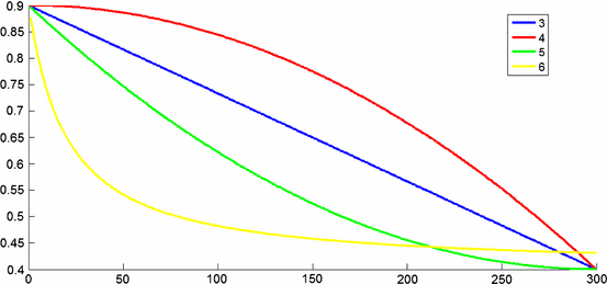
In this formula, \( \omega_{\text{start}} \) is the initial inertia weight, \( \omega_{\text{end}} \) is the inertia weight in the maximum iterations, \( k \) is the current number of iterations and \( T_{\rm max } \) is the maximum number of iterations. Generally speaking, the algorithm has the best performance when \( \omega_{\text{start}} = 0.9,\;\;\omega_{\text{end}} = 0.4 \). In this way, as iteration increases, the inertia weight decreases from 0.9 to 0.4 linearly. A bigger inertia weight in the early iteration can help the algorithm maintain stronger global search ability while a smaller one in the late iteration is good for the algorithm to conduct local search more accurately [12]. The selection of common inertia weight includes the following kinds.
The dynamic changes of these several \( w \) are shown in Fig. 1.
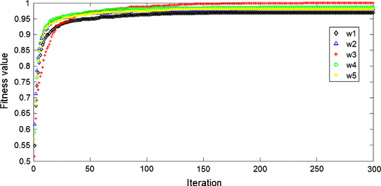
The parameters of the algorithm are set as follows: the population size is 20 and the number of evolutions is 300. In every experiment, operate 100 times and take the mean value as the final results. Under the above setting of parameters, solve the function with 5 \( w \) methods and analyze their convergence accuracy and velocity. The evolutionary curves and operation results of every \( w \) algorithm are shown in Fig. 2 and Table 1.
In PSO, the inertia weight is used to balance the global and local search capabilities. The inertia weight has the greatest impact on the performance of the PSO algorithm, and the larger inertia weight is more inclined to global search, while the smaller inertia weight is suitable for local search. It can be seen from Fig. 2 and Table 1 that although PSO with unchanged inertia weight \( \omega \) has a faster convergence velocity, it is easy to get trapped in local optimum in the late period and it has a low accuracy. The several algorithms with dynamically changing \( \omega \) are slow in the initial convergence, but they have strong local search ability in the late period, which is good to jump out of local optimum and obtain the optimal solution and it improves the accuracy. As for the method with dynamical change in \( \omega \) in Formula (4), \( \omega \) changes slowly in the early period and its value is big, so it maintains the global search ability of the algorithm, in the late period, \( \omega \) changes rapidly, which greatly enhances its local optimization ability [13].
3 Basic principles of simulated annealing
SA not only accepts good solution in the search process, but it also accepts bad solution at a certain probability. In the meanwhile, such jumping probability is under the control of temperature. In other words, the probability decreases as the temperature drops and when the temperature is close to 0, the probability is also close to 0. Therefore, SA has probability jumping ability in its search process and it can effectively avoid getting trapped in local minimums. SA is converged to globally optimal solution at the probability of 1 under certain conditions and its physical annealing process includes the following three parts [14].
-
(1)
Heating process, its purpose is to enhance the thermal movement of the particle to make it deviate from the equilibrium position. When the temperature is high enough, the solid is melted into liquid to eliminate the non-uniform stage in the system.
-
(2)
Isothermal process, for the closed system which exchanges heat with the surrounding environment but its temperature remains the same, the spontaneous changes in the state of the system proceeds along the direction with reduced free energy. When the free energy is the minimal, the system reaches the equilibrium state.
-
(3)
Cooling process, it weakens the thermal movement of the particle, lowers the energy of the system and obtains the crystallographic structure.
Among them, the heating process corresponds to the preset initial temperature of the algorithm, the isothermal process to the Metropolis sampling process and the cooling process to the decrease of the control parameters. The energy change here is the objective function and the optimal solution to be obtained is the lowest energy state. Metropolis criterion is that SA accepts bad solution at a certain probability, in this way, the algorithm can jump out of local optimum.
Implementation steps of SA are as follows.
-
(1)
Initialize the annealing temperature \( T_{k} \) (make \( k = 0 \)), randomly produce the initial solution \( x_{0} \), take an initial temperature \( T_{0} \) big enough and select the initial solution \( S_{1} , \) confirm the number of iterations for every \( T \), i.e. the Metropolis chain length \( L. \)
-
(2)
For the current temperature \( T \) and \( k = 1,2, \ldots ,L \), repeat the following operations under the temperature of \( T_{k} \) until it reaches the equilibrium state at temperature \( T_{k} \).
-
①
Produce new feasible solution \( x^{\prime} \) in the neighborhood of solution \( x \).
-
②
Calculate the difference \( \Delta f \) between the objective function \( f(x^{\prime}) \) of \( x^{\prime} \) and the objective function \( f(x) \) of \( x \).
-
③
Receive \( x^{\prime}, \) at the probability of \( \hbox{min} \{ 1,\exp ( - \Delta f/T_{k} )\} > random[0,1] \), here, \( random[0,1] \) is a random number within the scope of [0,1].
-
(3)
Annealing operation, produce a new solution \( S_{2} \) through stochastic disturbance on the current solution \( S_{1} \), \( T_{k + 1} = CT_{k} ,k \leftarrow k + 1 \), and \( C \in (0,1) \). If convergence criterion is met, the annealing process ends.
-
(4)
Calculate the increment \( {\text{d}}f = f(S_{2} ) - f(S_{1} ), \) of \( S_{2} \), here, \( f(S_{1} ) \) is the cost function of \( S_{1} \).
The annealing temperature control the solving process move towards the optimization direction of the optimal value and it accepts bad solution at the probability of \( \exp ( - \Delta f/T_{k} ) \). Therefore, this algorithm can jump out of local extremums. As long as the initial temperature is high enough and the annealing process is slow enough, the algorithm can converge to the globally optimal solution.
-
(5)
If \( df < 0, \) accept \( S_{2} \) as the new current solution, namely \( S_{1} = S_{2} \), otherwise, calculate the acceptance probability \( \exp ( - df/T) , \) of \( S_{2} \), namely to produce the random number rand uniformly distributed within the range of (0, 1). If \( \exp ( - df/T) > {\text{rand}} \), also take \( S_{2} \) as the new current solution, namely \( S_{1} = S_{2} \), otherwise, maintain the current solution \( S_{1} . \)
-
(6)
If the end condition is met, output the current solution \( S_{1} \) as the optimal solution, if not met, return to Step (2) after attenuating \( T \) according to the attenuation function.
The above steps are called as Metroplis process, the iteration process of “production of new solution-judgment-acceptance or abandonment” proceeds until the equilibrium point under that temperature is reached. Among the globally optimal solutions to the combinatorial optimization problems obtained by SA, one solution \( i \) and its objective function \( f(i) \) correspond to a micro state \( i \) and its energy \( E_{i} \) of the solid respectively and the control parameter \( T \) which decreases with the algorithm serves as the temperature of solid annealing process [15, 16].
4 Particle swarm optimization with constriction factor based on simulated annealing
The steps of the mixed algorithm of this paper are classified as follows.
-
1.
Randomly initialize the position and velocity of every particle and calculate the value of the objective function of every particle of the swarm.
-
2.
Evaluate the fitness of every particle and update its Pbest and Gbest, store the position and fitness of the particle in its individual extremum \( p_{\text{best}} \) and the position and fitness of the individual with the best fitness among all \( p_{\text{best}} \) in the global extremum \( g_{\text{best}} \).
-
3.
Identify the initial temperature and confirm the fitness of every particle \( p_{i} \) in the current temperature.
$$ {\text{TF}}(p_{i} ) = \frac{{{\text{e}}^{{ - (f(p_{i} ) - f(p_{g} ))/t}} }}{{\sum\nolimits_{i = 1}^{N} {{\text{e}}^{{ - (f(p_{i} ) - f(p_{g} ))/t}} } }} $$(7)
Adopt the Roulette strategy to confirm a certain globally optimal alternative value \( p_{g}^{\prime } \) from all \( p_{i} \), which is good to overcome the shortcomings of particle swarm optimization.
(4) Calculate the objective value of the particle and update \( p_{\text{best}} \) and \( g_{\text{best}} \). Then, lower the temperature. The velocity and position update formulas of particle swarm optimization with constriction factor are shown as follows.
Here, constriction factor is \( \chi = \frac{2}{{\left| {2 - C - \sqrt {C^{2} - 4C} } \right|}},C = c_{1} + c_{2} ,C > 4. \). As the velocity update formula (8) uses the best position of the swarm, all particles will fly towards this best position. If the best position is located in the local minimum, all particles will move toward the locally minimum solution, resulting in bad dispersibility of search and weak global search ability. Therefore, in order to enhance the algorithm’s ability to avoid getting trapped in local minimum solution, select a position from the many \( p_{i} \), marked as \( \dot{p}_{g} , \), to replace the \( p_{i} . \) in the update formula. Then, Formula (8) has become the following.
The \( p_{i} \) with excellent performance shall be given a higher probability to be selected, \( p_{i} \) is a special solution worse than \( p_{g} \) so that the jumping probability from \( p_{i} \) to \( p_{g} \) at the temperature \( t \) can be calculated, namely \( {\text{e}}^{{ - (f_{pi} - f_{pg} )/t}} \). Here, \( f \) represents the value of the objective function. If the second jumping probability is seen as the fitted value of \( p_{i} \), replace the probability of \( p_{g} \) with \( p_{i} \).
(5) The initial temperature and the temperature-lowing methods have certain impact on the algorithm. The following temperature-lowering method is adopted.
The jumping probability, namely \( {\text{e}}^{{ - (f_{pi} - f_{pg} )/t}}, \) can be calculated according to Formula (11).
In this formula, \( N \) is the population size.
(6) When the algorithm has met the end conditions, stop the search and output the result, otherwise, return to Step (4) and continue.
The algorithm of this paper doesn’t need to adjust too many parameters and the setting of these parameters depends on experience to a large extent. Combining the results obtained from different iteration steps and different sizes of particle swarm, for the algorithm of this paper, in order to obtain solution of high accuracy, the key is the property matching between parameters.
5 Experimental test
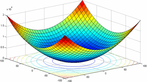
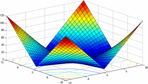
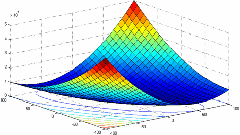
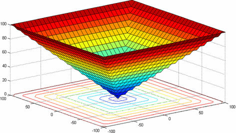
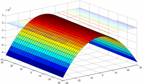
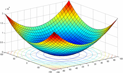
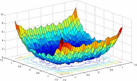
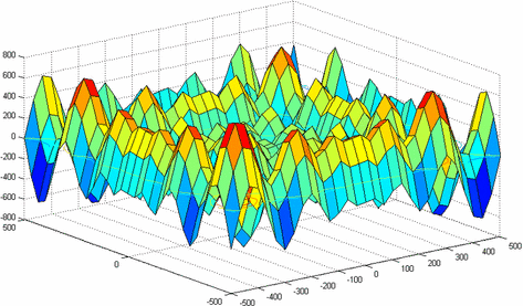
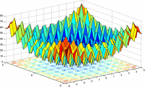
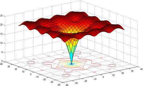
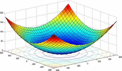
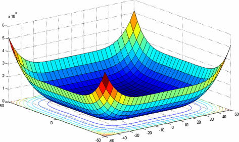
In our experiment, 12 test functions have been used, hoping to compare the optimization performance of SA-CPSO and LDIW-PSO thoroughly. The specific forms of these 12 test functions are listed in Table 2, among them, \( f_{1} - f_{5} \) are uni-modal problems, \( f_{6} \) is a discontinuous staircase function with only one minimum, \( f_{7} \) is a fourth-order noise function and \( f_{8} - f_{12} \) are multi-modal functions, the local optimums of which increase with the increase of dimensions exponentially. These are the most difficult problems for many optimization algorithms. We have adopted SA-CPSO and LDIW-PSO to complete the evaluation of these 12 test function at the same computation N = 20 (Figs. 3, 4, 5, 6, 7, 8, 9, 10, 11, 12, 13, 14).
-
1.
Uni-modal function
In functions \( f_{1} - f_{5} \), there only contains one optimal solution in the fitness landscape. The purpose to use uni-modal functions \( f_{1} - f_{5} \) is to compare the convergence velocity of SA-CPSO and LDIW-PSO and the accuracy of the solutions obtained. The statistical results of 20 operations are summarized in Table 3. It can be seen from Table 3 that SA-CPSO is better than LDIW-PSO in terms of the performance in uni-modal functions and its convergence velocity and optimization result is far better than those of LDIW-PSO. It is especially true in function \( f_{4} \) which is proved a big challenge to PSO. SA-CPSO can search a more accurate solution, it has proven that SA-CPSO has strong capabilities to solve complex uni-modal problems.
Table 3 Comparison of mean value and standard deviation of solutions -
2.
Special function
It can be concluded from Table 4 that function \( f_{6} \) is a classical staircase problem, which has many discontinuous breakpoints. For \( f_{6} \), it is inevitable for the classical mathematical approximation algorithm to be ineffective. Both SA-CPSO and LDIW-PSO have demonstrated excellent convergence results in \( f_{6} \), a discontinuous staircase function. For the fourth-order noise function \( f_{7} \), SA-CPSO has a better accuracy than LDIW-PSO, but its standard deviation is not as good as that of LDIW-PSO. Therefore, for the problems which are difficult to be solved by classical mathematical approximation algorithm, both SA-CPSO and LDIW-PSO can lead to excellent optimization results.
Table 4 Comparison of mean value and standard deviation of solutions -
3.
Multi-modal function
It can be seen from Table 5 that the functions with numerous locally optimal solutions are universally acknowledged optimization problems with difficulty. \( f_{8} - f_{12} \) are these functions, their locally optimal solutions increase rapidly with the increase of dimensions. Table 5 has recorded the statistic optimization results of 20 computations. Overall, SA-CPSO has better optimization on all 5 multi-modal problems than LDIW-PSO, as evidenced by the comparison indexes. For the test problem \( f_{12} \), the mean value and standard deviation of SA-CPSO are bigger. But as a whole, SA-CPSO has a better performance and it has found the optimal solutions to most problems, which has shown that SA-CPSO is effective in multi-modal problems.
Table 5 Comparison of mean value and standard deviation of solutions
The above test results have demonstrated that the algorithm of this paper has a better performance compared with other similar algorithms. Because the simulated annealing algorithm is hopping, it is not easy to fall into the local minima, and has the advantages of strong local search ability and fast convergence speed near the optimal value. Therefore, the simulated annealing algorithm integrates it into the PSO structure, improves the convergence speed of the algorithm by improving the space exploration ability of the particle, and improves the ability of PSO to get out of the local extreme points. The convergence accuracy of the algorithm is improved. As the evolution proceeds, the temperature of this algorithm gradually falls and its probability to accept a bad solution gradually decreases, so its convergence performance is improved. This algorithm has not only basically maintained the enhanced global optimization ability of particle swarm optimization, but it has also accelerated its acceleration velocity and enhanced the convergence accuracy. In engineering applications, about the selection of algorithm parameters, the method that selects certain kinds of parameters is not necessary to be better than other parameters. On the contrary, it has to be combined with practical problems and get familiar with the convergence features of specific problems in the iteration process. To select the parameters and the changes correctly can avoid getting trapped in local optimum.
6 Conclusions
PSO is a kind of simple and effective stochastic global optimization technique, it adopts the evolutionary advantage produced by the information sharing mechanism between biological communities to search for the optimal solution through the collaboration between individuals. This paper has brought the Metropolis criterion of simulated annealing algorithm into the particle swarm optimization with constriction factor. First, it analyzes the impact the parameters have on the algorithm performance and the convergence, efficiency and parameter selection in different forms. On this basis, it proposes a cooperative particle swarm optimization with constriction factor based on simulated annealing, stages the principles and steps of the algorithm, conducts comparative analysis in sensitivity of parameters and performance of algorithm and demonstrates the convergence of the algorithm. The algorithm of this paper basically is simple and easy to implement, just like particle swarm optimization, but it overcomes the defects that standard particle swarm optimization is low in the follow-up iteration and easy to get trapped in locally optimal solution and it improves its ability to get rid of local extremum. With its sudden jumping in the search process, it can effectively avoid getting trapped into local minimum and it improves the convergence speed and accuracy. Last but not least, this paper uses test functions to analyze the performance of the algorithm of this paper and the experiment data has shown that in the optimization of high-dimensional, multi-modal and complex problems, the algorithm of this paper has improved the convergence performance and better balanced global convergence ability and local search capacity. It has not only higher convergence accuracy and faster convergence velocity, but also better stability. The future research on PSO is mainly about how to choose the inertia weight factor, which plays a decisive role in the result of the whole algorithm. Therefore, the choice of inertia weight needs to be studied emphatically. In addition, how to combine PSO with other optimization algorithms is very important for PSO to jump out of local extremum and speed up convergence.
References
Brusco MJ (2014) A comparison of simulated annealing algorithms for variable selection in principal component analysis and discriminant analysis. Comput Stat Data Anal 77(9):38–53
Lee KH, Kim KW (2015) Performance comparison of particle swarm optimization and genetic algorithm for inverse surface radiation problem. Int J Heat Mass Transf 88(9):330–337
Silva Filho TM, Pimentel BA, Souza RMCR, Oliveira ALI (2015) Hybrid methods for fuzzy clustering based on fuzzy C-means and improved particle swarm optimization. Expert Syst Appl 42(17–18):6315–6328
Balaji AN, Porselvi S (2014) Artificial immune system algorithm and simulated annealing algorithm for scheduling batches of parts based on job availability model in a multi-cell flexible manufacturing system. Procedia Eng 97:1524–1533
Hamzadayi A, Yildiz G (2013) A simulated annealing algorithm based approach for balancing and sequencing of mixed-model U-lines. Comput Ind Eng 66(11):1070–1084
Zaji AH, Bonakdari H, Shamshirband S, Qasem SN (2015) Potential of particle swarm optimization based radial basis function network to predict the discharge coefficient of a modified triangular side weir. Flow Meas Instrum 45(10):404–407
Lou I, Xie Z, Ung WK, Mok KM (2015) Integrating support vector regression with particle swarm optimization for numerical modeling for algal blooms of freshwater. Appl Math Model 39(10):5907–5916
Soares S, Antunes CH, Araújo R (2013) Comparison of a genetic algorithm and simulated annealing for automatic neural network ensemble development. Neurocomputing 121(11):498–511
Chambari A, Najafi AA, Rahmati SHA, Karimi A (2013) An efficient simulated annealing algorithm for the redundancy allocation problem with a choice of redundancy strategies. Reliab Eng Syst Saf 119(11):158–164
Jadoun VK, Gupta N, Niazi KR, Swarnkar A (2015) Multi-area economic dispatch with reserve sharing using dynamically controlled particle swarm optimization. Int J Electr Power Energy Syst 73(12):743–756
Örkcü HH, Özsoy VS, Aksoy E, Dogan MI (2015) Estimating the parameters of 3-p weibull distribution using particle swarm optimization: a comprehensive experimental comparison. Appl Math Comput 268(10):201–226
Askarzadeh A, dos Santos Coelho L (2015) Using two improved particle swarm optimization variants for optimization of daily electrical power consumption in multi-chiller systems. Appl Therm Eng 89(10):640–646
Tatsumi K, Ibuki T, Tanino T (2015) Particle swarm optimization with stochastic selection of perturbation-based chaotic updating system. Appl Math Comput 269(10):904–929
Dai M, Tang D, Giret A, Salido MA, Li WD (2013) Energy-efficient scheduling for a flexible flow shop using an improved genetic-simulated annealing algorithm. Robot Comput Integr Manuf 29(10):418–429
Örkcü HH (2013) Subset selection in multiple linear regression models: a hybrid of genetic and simulated annealing algorithms review article. Appl Math Comput 219(8):11018–11028
Yannibelli V, Amandi A (2013) Hybridizing a multi-objective simulated annealing algorithm with a multi-objective evolutionary algorithm to solve a multi-objective project scheduling problem. Expert Syst Appl 40(6):2421–2434
Acknowledgement
This work was supported by the National Social Science Foundation of China (No. 16BGL145).
Author information
Authors and Affiliations
Corresponding author
Ethics declarations
Conflict of interest
We declare that we have no financial and personal relationships with other people or organizations that can inappropriately influence our work, there is no professional or other personal interest of any nature or kind in any product, service and/or company that could be construed as influencing the position presented in, or the review of, the manuscript entitled.
Rights and permissions
Open Access This article is distributed under the terms of the Creative Commons Attribution 4.0 International License (http://creativecommons.org/licenses/by/4.0/), which permits unrestricted use, distribution, and reproduction in any medium, provided you give appropriate credit to the original author(s) and the source, provide a link to the Creative Commons license, and indicate if changes were made.
About this article
Cite this article
Wu, Z., Zhang, S. & Wang, T. A cooperative particle swarm optimization with constriction factor based on simulated annealing. Computing 100, 861–880 (2018). https://doi.org/10.1007/s00607-018-0625-6
Received:
Accepted:
Published:
Issue Date:
DOI: https://doi.org/10.1007/s00607-018-0625-6

