LP-based approximations for disjoint bilinear and two-stage adjustable robust optimization

Abstract

We consider the class of disjoint bilinear programs $\max \, \{ {\textbf{x}}^T{\textbf{y}} \mid {\textbf{x}} \in {\mathcal {X}}, \;{\textbf{y}} \in {\mathcal {Y}}\}$ where ${\mathcal {X}}$ and ${\mathcal {Y}}$ are packing polytopes. We present an $O(\frac{\log \log m_1}{\log m_1} \frac{\log \log m_2}{\log m_2})$-approximation algorithm for this problem where $m_1$ and $m_2$ are the number of packing constraints in ${\mathcal {X}}$ and ${\mathcal {Y}}$ respectively. In particular, we show that there exists a near-optimal solution $(\tilde{{\textbf{x}}}, \tilde{{\textbf{y}}})$ such that $\tilde{{\textbf{x}}}$ and $\tilde{{\textbf{y}}}$ are “near-integral". We give an LP relaxation of the problem from which we obtain the near-optimal near-integral solution via randomized rounding. We show that our relaxation is tightly related to the widely used reformulation linearization technique. As an application of our techniques, we present a tight approximation for the two-stage adjustable robust optimization problem with covering constraints and right-hand side uncertainty where the separation problem is a bilinear optimization problem. In particular, based on the ideas above, we give an LP restriction of the two-stage problem that is an $O(\frac{\log n}{\log \log n} \frac{\log L}{\log \log L})$-approximation where L is the number of constraints in the uncertainty set. This significantly improves over state-of-the-art approximation bounds known for this problem. Furthermore, we show that our LP restriction gives a feasible affine policy for the two-stage robust problem with the same (or better) objective value. As a consequence, affine policies give an $O(\frac{\log n}{\log \log n} \frac{\log L}{\log \log L})$-approximation of the two-stage problem, significantly generalizing the previously known bounds on their performance.

Appendices

Appendix A: Chernoff bounds

Proof of Chernoff bounds (a)

From Markov’s inequality we have for all $t>0$,

$$\begin{aligned} {\mathbb {P}}( {\varXi } \ge (1+ \delta ) s ) = {\mathbb {P}}( e^{t{\varXi }} \ge e^{t(1+\delta )s} ) \le \frac{{\mathbb {E}}(e^{t{\varXi }})}{e^{t(1+\delta )s}}. \end{aligned}$$

Denote $p_i$ the parameter of the Bernoulli ${\chi }_i$. By independence, we have

$$\begin{aligned} {\mathbb {E}}(e^{t{\varXi }})= \prod _{i=1}^r {\mathbb {E}} (e^{t \epsilon _i {\chi }_i}) = \prod _{i=1}^r \left( p_i e^{t \epsilon _i }+1-p_i \right) \le \prod _{i=1}^r \exp \left( p_i (e^{t \epsilon _i }-1) \right) \end{aligned}$$

where the inequality holds because $1+x \le e^x$ for all $x \in {\mathbb {R}}$. By taking $t=\ln ( 1+ \delta ) >0$, the right hand side becomes

$$\begin{aligned} \prod _{i=1}^r \exp \left( p_i ((1+\delta )^{ \epsilon _i }-1) \right) \le \prod _{i=1}^r \exp \left( p_i \delta \epsilon _i \right) =\exp \left( \delta \cdot {\mathbb {E}}({\varXi } ) \right) \le e^{\delta s} , \end{aligned}$$

where the first inequality holds because $(1+x)^{\epsilon } \le 1+ \alpha x$ for any $x \ge 0$ and $\epsilon \in [0,1]$ and the second one because $s \ge {\mathbb {E}}({\varXi } )= \sum _{i=1}^r \epsilon _i p_i$. Hence, we have

$$\begin{aligned} {\mathbb {E}}(e^{t{\varXi }}) \le e^{\delta s}. \end{aligned}$$

On the other hand,

$$\begin{aligned} e^{t(1+\delta )s} = (1+\delta ) ^{(1+\delta )s}. \end{aligned}$$

Therefore,

$$\begin{aligned} {\mathbb {P}}( {\varXi } \ge (1+ \delta ) s ) \le \left( \frac{e^{\delta s}}{(1+\delta ) ^{(1+\delta )s}} \right) =\left( \frac{e^{\delta }}{(1+\delta )^{1+\delta } } \right) ^s. \end{aligned}$$

$\square$

Proof of Chernoff bounds (b)

From Markov’s inequality we have for all $t< 0$,

$$\begin{aligned} {\mathbb {P}}( {\varXi } \le (1- \delta ) {\mathbb {E}}({\varXi }) ) = {\mathbb {P}}( e^{t{\varXi }} \ge e^{t(1-\delta ){\mathbb {E}}({\varXi })} ) \le \frac{{\mathbb {E}}(e^{t{\varXi }})}{e^{t(1-\delta ) {\mathbb {E}}({\varXi })}}. \end{aligned}$$

Denote $p_i$ the parameter of the Bernoulli ${\chi }_i$. By independence, we have

$$\begin{aligned} {\mathbb {E}}(e^{t{\varXi }})= \prod _{i=1}^r {\mathbb {E}} (e^{t \epsilon _i {\chi }_i}) = \prod _{i=1}^r \left( p_i e^{t \epsilon _i }+1-p_i \right) \le \prod _{i=1}^r \exp \left( p_i (e^{t \epsilon _i }-1) \right) , \end{aligned}$$

where the inequality holds because $1+x \le e^x$ for all $x \in {\mathbb {R}}$. We take $t=\ln ( 1- \delta ) < 0$. We have $t \le - \delta$, hence,

$$\begin{aligned} \prod _{i=1}^r \exp \left( p_i (e^{ t\epsilon _i }-1) \right) =\prod _{i=1}^r \exp \left( p_i ((1-\delta )^{ \epsilon _i }-1) \right) \le \prod _{i=1}^r \exp \left( -p_i \delta \epsilon _i \right) , \end{aligned}$$

where the inequality holds because $(1-x)^{\epsilon } \le 1- \epsilon x$ for any $0< x <1$ and $\epsilon \in [0,1]$. Therefore,

$$\begin{aligned} {\mathbb {E}}(e^{t{\varXi }}) \le \prod _{i=1}^r \exp \left( -p_i \delta \epsilon _i \right) = e^{-\delta {\mathbb {E}}({\varXi })}. \end{aligned}$$

On the other hand,

$$\begin{aligned} e^{t(1-\delta ) {\mathbb {E}}({\varXi })} = (1-\delta ) ^{(1-\delta ){\mathbb {E}}({\varXi })}. \end{aligned}$$

Therefore,

$$\begin{aligned} {\mathbb {P}}( {\varXi } \le (1- \delta ) {\mathbb {E}}({\varXi }) ) \le \left( \frac{e^{-\delta {\mathbb {E}}({\varXi })}}{(1-\delta ) ^{(1-\delta ){\mathbb {E}}({\varXi })}} \right) =\left( \frac{e^{-\delta }}{(1-\delta )^{1-\delta } } \right) ^{{\mathbb {E}}({\varXi })}. \end{aligned}$$

Finally, we have for any $0<\delta < 1$,

$$\begin{aligned} \ln (1- \delta ) \ge - \delta + \frac{\delta ^2}{2} \end{aligned}$$

which implies

$$\begin{aligned} (1- \delta ) \cdot \ln (1- \delta ) \ge - \delta + \frac{\delta ^2}{2} \end{aligned}$$

and consequently

$$\begin{aligned} \left( \frac{e^{-\delta }}{(1-\delta )^{1-\delta } } \right) ^{{\mathbb {E}}({\varXi })} \le e^{ \frac{-{\delta }^2 {\mathbb {E}}({\varXi })}{2}}. \end{aligned}$$

$\square$

Appendix B: Proof of Theorem 4

Our proof uses a polynomial time transformation from the Monotone Not-All-Equal 3-satisfiability (MNAE3SAT) NP-complete problem (Schaefer [37]). In the (MNAE3SAT), we are given a collection of Boolean variables and a collection of clauses, each of which combines three variables. (MNAE3SAT) is the problem of determining if there exists a truth assignment where each close has at least one true and one false literal. This is a subclass of the Not-All-Equal 3-satisfiability problem where the variables are never negated.

Consider an instance ${\mathcal {I}}$ of (MNAE3SAT), let ${\mathcal {V}}$ be the set of variables of ${\mathcal {I}}$ and let ${\mathcal {C}}$ be the set of clauses. Let ${\textbf{A}} \in \{0,1\}^{|{\mathcal {C}}| \times |{\mathcal {V}}|}$ be the variable-clause incidence matrix such that for every variable $v \in {\mathcal {V}}$ and clause $c \in {\mathcal {C}}$ we have $A_{cv}=1$ if and only if the variable v belongs to the clause c. We consider the following instance of CDB denoted by ${\mathcal {I}}'$,

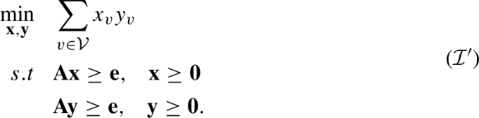
Let $z_{{\mathcal {I}}'}$ denote the optimum of ${\mathcal {I}}'$. We show that ${\mathcal {I}}$ has a truth assignment where each clause has at least one true and one false literal if and only if $z_{{\mathcal {I}}'} = 0$.

First, suppose $z_{{\mathcal {I}}'} = 0$. Let $({\textbf{x}}, {\textbf{y}})$ be an optimal solution of ${\mathcal {I}}'$. Let $\tilde{{\textbf{x}}}$ such that ${\tilde{x}}_v = \mathbb {1}_{\{x_v > 0\}}$ for all $v \in {\mathcal {V}}$. We claim that $(\tilde{{\textbf{x}}}, {\textbf{e}} - \tilde{{\textbf{x}}})$ is also an optimal solution of ${\mathcal {I}}$. In fact, for all $c \in {\mathcal {C}}$, we have,

$$\begin{aligned} \sum _{v \in {\mathcal {V}}} A_{cv} x_v \ge 1, \end{aligned}$$

hence,

$$\begin{aligned} \sum _{v \in {\mathcal {V}} } A_{cv} \min (x_v, 1) \ge 1, \end{aligned}$$

since the entries of ${\textbf{A}}$ are in $\{0,1\}$. Therefore,

$$\begin{aligned} \sum _{v \in {\mathcal {V}} } A_{cv} {\tilde{x}}_v \ge \sum _{v \in {\mathcal {V}} } A_{cv} \min (x_v, 1) \ge 1. \end{aligned}$$

Finally, ${\textbf{A}} \tilde{{\textbf{x}}} \ge {\textbf{e}}$. Similarly, for all $c \in {\mathcal {C}}$ we have,

$$\begin{aligned} \sum _{v \in {\mathcal {V}} } A_{cv} y_v \ge 1, \end{aligned}$$

hence,

$$\begin{aligned} \sum _{v \in {\mathcal {V}} } A_{cv} \min (y_v, 1) \ge 1, \end{aligned}$$

since the entries of ${\textbf{A}}$ are in $\{0,1\}$. Therefore,

$$\begin{aligned} \sum _{v \in {\mathcal {V}} } A_{cv} (1- {\tilde{x}}_v) \ge \sum _{v \in {\mathcal {V}} } A_{cv} (1- {\tilde{x}}_v) \min (y_v, 1) = \sum _{v \in {\mathcal {V}} } A_{cv} \min (y_v, 1) \ge 1. \end{aligned}$$

where the equality follows from the fact that $y_v = 0$ for all v such that ${\tilde{x}}_v = 1$. Note that $\sum _{v \in {\mathcal {V}} } x_vy_v = z_{{\mathcal {I}}'} = 0$. This implies that ${\textbf{A}}({\textbf{e}} - \tilde{{\textbf{x}}}) \ge {\textbf{e}}$. Therefore, $(\tilde{{\textbf{x}}}, {\textbf{e}} - \tilde{{\textbf{x}}})$ is a feasible solution of ${\mathcal {I}}'$ with objective value $\sum _{v \in {\mathcal {V}} } {\tilde{x}}_v(1-{\tilde{x}}_v) = 0 = z_{{\mathcal {I}}'}$. It is therefore an optimal solution. Consider now the truth assignment where a variable v is set to be true if and only if ${\tilde{x}}_v = 1$. We show that each clause in such assignment has at least one true and one false literal. In particular, consider a clause $c \in {\mathcal {C}}$, since,

$$\begin{aligned} \sum _{v \in {\mathcal {V}} } A_{cv} {\tilde{x}}_v \ge 1, \end{aligned}$$

there must be a variable v belonging to the clause c such that ${\tilde{x}}_v = 1$. Similarly, since

$$\begin{aligned} \sum _{v \in {\mathcal {V}}} A_{cv} (1-{\tilde{x}}_v) \ge 1, \end{aligned}$$

there must be a variable v belonging to the clause c such that ${\tilde{x}}_v = 0$. This implies that our assignment is such that the clause c has at least one true and one false literal.

Conversely, suppose there exists a truth assignment of ${{\mathcal {I}}}$ where each clause has at least one false and one true literal. We show that $z_{{\mathcal {I}}'} = 0$. In particular, define ${\textbf{x}}$ such that for all $v \in {\mathcal {V}}$ we have $x_v = 1$ if and only if v is assigned true. We have for all $c \in {\mathcal {C}}$,

$$\begin{aligned} \sum _{v \in {\mathcal {V}} } A_{cv} x_v \ge 1, \end{aligned}$$

since at least one of the variables of c is assigned true. And,

$$\begin{aligned} \sum _{v \in {\mathcal {V}} } A_{cv} (1-x_v) \ge 1, \end{aligned}$$

since at least one of the variables of c is assigned false. Hence, $({\textbf{x}}, {\textbf{e}} - {\textbf{x}})$ is feasible for ${\mathcal {I}}'$ with objective value $\sum _{v \in {\mathcal {V}}} x_v(1-x_v) = 0$. It is therefore an optimal solution and $z_{{\mathcal {I}}'} = 0$.

If there exists a polynomial time algorithm approximating CDB to some finite factor, such an algorithm can be used to decide in polynomial time whether $z_{{\mathcal {I}}'} = 0$ or not, which is equivalent to solving ${\mathcal {I}}$ in polynomial time; a contradiction. $\square$

Appendix C: Derivation of the first level relaxation of the RLT hierarchy

Let us begin by writing PDB in the following equivalent epigraph form,

$$\begin{aligned} \max _{{\textbf{x}}, {\textbf{y}}, {\textbf{u}}, {\textbf{v}}, {\textbf{w}}} \quad&\sum _{i=1}^n \theta _i \gamma _i u_{ii}\\&u_{ij} \le x_i y_j, \quad \forall i, j\\&v_{i,j} \le x_i x_j, \quad \forall i, j\\&w_{i,j} \le y_i y_j, \quad \forall i, j\\&\sum _{i=1}^n \theta _i{\textbf{P}}_ix_i \le {\textbf{p}},\\&\sum _{i=1}^n \gamma _i{\textbf{Q}}_iy_i \le {\textbf{q}},\\&0 \le x_i \le 1, \quad 0 \le y_i \le 1, \quad \forall i. \end{aligned}$$

Reformulation phase. In the reformulation phase we add to the above program the polynomial constraints we get from multiplying all the linear constraints by linear constraints by $x_i$, $y_i$, $(1-x_i)$ and $(1-y_i)$ for all $i \in [n]$. We get the following equivalent formulation of PDB,

$$\begin{aligned} \max _{{\textbf{x}}, {\textbf{y}}, {\textbf{u}}, {\textbf{v}}, {\textbf{w}}} \quad&\sum _{i=1}^n \theta _i \gamma _j u_{ii}\\&u_{ij} \le x_i y_j, \quad \forall i, j,\\&v_{i,j} \le x_i x_j, \quad \forall i, j\\&w_{i,j} \le y_i y_j, \quad \forall i, j\\&\sum _{j=1}^n \theta _j{\textbf{P}}_jx_j \le {\textbf{p}},\\&\sum _{j=1}^n \theta _j{\textbf{P}}_{j}x_jx_i \le {\textbf{p}}x_i,\\&\sum _{j=1}^n \theta _j{\textbf{P}}_{j}(x_j- x_jx_i) \le {\textbf{p}} (1- x_i)\\&\sum _{j=1}^n \theta _j{\textbf{P}}_{j}x_jy_i \le {\textbf{p}}y_i,\\&\sum _{j=1}^n \theta _j{\textbf{P}}_{j}(x_j- y_ix_j) \le {\textbf{p}} (1- y_i)\\&\sum _{j=1}^n \gamma _j{\textbf{Q}}_jy_j \le {\textbf{q}},\\&\sum _{j=1}^n \gamma _j{\textbf{Q}}_{j}y_jx_i \le {\textbf{q}}x_i,\\&\sum _{j=1}^n \gamma _j{\textbf{Q}}_{j}(y_j- y_jx_i) \le {\textbf{p}} (1- x_i)\\&\sum _{j=1}^n \gamma _j{\textbf{Q}}_{j}y_jy_i \le {\textbf{q}}y_i,\\&\sum _{j=1}^n \gamma _j{\textbf{Q}}_{j}(y_j- y_jy_i) \le {\textbf{p}} (1- y_i)\\&0 \le x_i \le 1, \quad 0 \le y_i \le 1, \quad \forall i\\&x_ix_j \le x_i, \quad x_ix_j \le x_j,\\&y_iy_j \le y_i, \quad y_iy_j \le y_j,\\&x_iy_j \le x_i, \quad x_iy_j \le y_j, \end{aligned}$$

Linearization phase. We replace the bilinear terms $x_iy_j$, $x_ix_j$ and $y_iy_j$ in the above LP with their respective lower-bounds $u_{ij}$, $v_{i,j}$, $w_{i,j}$. We get the following linear relaxation of PDB,

$$\begin{aligned} \max _{{\textbf{x}}, {\textbf{y}}, {\textbf{u}}, {\textbf{v}}, {\textbf{w}}} \quad&\sum _{i=1}^n \theta _i \gamma _j u_{ii}\\&\sum _{j=1}^n \theta _j{\textbf{P}}_jx_j \le {\textbf{p}},\\&\sum _{j=1}^n \theta _j{\textbf{P}}_{j}v_{i,j} \le {\textbf{p}}x_i,\\&\sum _{j=1}^n \theta _j{\textbf{P}}_{j}(x_j- v_{i,j}) \le {\textbf{p}} (1- x_i)\\&\sum _{j=1}^n \theta _j{\textbf{P}}_{j}u_{ji} \le {\textbf{p}}y_i,\\&\sum _{j=1}^n \theta _j{\textbf{P}}_{j}(x_j- u_{ji}) \le {\textbf{p}} (1- y_i)\\&\sum _{j=1}^n \gamma _j{\textbf{Q}}_jy_j \le {\textbf{q}},\\&\sum _{j=1}^n \gamma _j{\textbf{Q}}_{j}u_{ij} \le {\textbf{q}}x_i,\\&\sum _{j=1}^n \gamma _j{\textbf{Q}}_{j}(y_j- u_{ij}) \le {\textbf{q}} (1- x_i)\\&\sum _{j=1}^n \gamma _j{\textbf{Q}}_{j}w_{i,j} \le {\textbf{q}}y_i,\\&\sum _{j=1}^n \gamma _j{\textbf{Q}}_{j}(y_j- w_{i,j}) \le {\textbf{q}} (1- y_i)\\&0 \le x_i \le 1, \quad 0 \le y_i \le 1, \quad \forall i\\&v_{i,j} \le x_i, \quad v_{i,j} \le x_j,\\&w_{i,j} \le y_i, \quad w_{i,j} \le y_j,\\&u_{ij} \le x_i, \quad u_{ij} \le y_j. \end{aligned}$$

The above LP is known as the first level relaxation of the RLT hierarchy. The above LP can be further simplified as follows: the constraints in ${\textbf{v}}$ and ${\textbf{w}}$ in the above are redundant and can be removed without loss of generality. In fact, for any feasible solution ${\textbf{x}}, {\textbf{y}}, {\textbf{u}}$ of the resulting LP, one can take $v_{i,j}=x_ix_j$ and $w_{i,j}=y_iy_j$ to get a feasible solution of the above LP with same cost, and conversely for every feasible solution ${\textbf{x}}, {\textbf{y}}, {\textbf{u}}, {\textbf{v}}, {\textbf{w}}$ of the above LP, the solution ${\textbf{x}}, {\textbf{y}}, {\textbf{u}}$ is a feasible solution of the resulting LP with same cost. Also, the first (resp. sixth) set of constraints in the above LP can be obtained by summing the fourth and fifth (resp. seventh and eighth) set of constraints and can therefore be removed as well. We get the following equivalent LP relaxation of PDB that we refer to in this paper as the first level relaxation of the RLT hierarchy,

$$\begin{aligned} \max _{{\textbf{x}}, {\textbf{y}}, {\textbf{u}}} \quad&\sum _{i=1}^n \theta _i \gamma _j u_{ii}\\&\sum _{j=1}^n \theta _j{\textbf{P}}_{j}u_{ji} \le {\textbf{p}}y_i,\\&\sum _{j=1}^n \theta _i{\textbf{P}}_{j}(x_j- u_{ji}) \le {\textbf{p}} (1- y_i)\\&\sum _{j=1}^n \gamma _j{\textbf{Q}}_{j}u_{ij} \le {\textbf{q}}x_i,\\&\sum _{j=1}^n \gamma _j{\textbf{Q}}_{j}(y_j- u_{ij}) \le {\textbf{q}} (1- x_i)\\&0 \le u_{ij} \le x_i \le 1, \quad 0 \le u_{ij} \le y_j \le 1. \end{aligned}$$

(FL-RLT)

Appendix D: Proof of Lemma 4

Let $\varvec{\omega }^*$ be an optimal solution of ${{\mathcal {Q}}^{\textsf{LP}}(\beta {\textbf{x}})}$, consider ${\tilde{\omega }}_1, \dots , {\tilde{\omega }}_m$ i.i.d. Bernoulli random variables such that ${\mathbb {P}}({\tilde{\omega }}_i = 1) = \omega ^*_i$ for all $i \in [m]$ and let $({\textbf{h}}, {\textbf{z}})$ such that $h_i = \frac{\gamma _i{\tilde{\omega }}_i}{\beta }$ and $z_i = \frac{\theta _i{\tilde{\omega }}_i}{\eta }$ for all $i \in [m]$. We show that $({\textbf{h}}, {\textbf{z}})$ satisfies the properties (5) with a constant probability. In particular, we have,

$$\begin{aligned} \begin{aligned} {\mathbb {P}}\left( \sum _{i=1}^m {\textbf{b}}_i z_i \nleq {\textbf{d}}\right)&= {\mathbb {P}}\left( \sum _{i=1}^m \theta _i{\textbf{b}}_i\frac{{\tilde{\omega }}_i}{\eta } \nleq {\textbf{d}}\right) \\&\le \sum _{j=1}^{n} {\mathbb {P}}\left( \sum _{i=1}^m \theta _i B_{ij}\frac{{\tilde{\omega }}_i}{\eta }> d_j\right) \\&= \sum _{j \in [n]: d_j> 0} {\mathbb {P}}\left( \sum _{i=1}^m \frac{\theta _i B_{ij}}{d_j}{\tilde{\omega }}_i> \eta \right) \\&\le \sum _{j \in [n]: d_j > 0} \left( \frac{e^{\eta -1}}{\eta ^{\eta }}\right) \\&\le n \frac{e^{\eta -1}}{\eta ^{\eta }}, \end{aligned} \end{aligned}$$

where the first inequality follows from a union bound on n constraints. The second equality holds because for all $j \in [n]$ such that $d_j = 0$ we have

$$\begin{aligned} {\mathbb {P}}\left( \sum _{i=1}^m \theta _i B_{ij}\frac{{\tilde{\omega }}_i}{\eta } > d_j\right) = 0. \end{aligned}$$

Note that $d_j = 0$ implies

$$\begin{aligned} \sum _{i=1}^m \theta _i B_{ij}\frac{\omega ^*_i}{\eta } = 0, \end{aligned}$$

by feasibility of $\varvec{\omega }^*$ in ${{\mathcal {Q}}^{\textsf{LP}}(\beta {\textbf{x}})}$. Therefore,

$$\begin{aligned} \sum _{i=1}^m \theta _i B_{ij}\frac{{\tilde{\omega }}_i}{\eta } = 0, \end{aligned}$$

almost surely. The second inequality follows from the Chernoff bounds (a) with $\delta = \eta - 1$ and $s=1$. In particular, $\frac{\theta _i B_{ij}}{d_j} \in [0,1]$ by definition of $\theta _i$ for all $i \in [m]$ and $j \in [n]$ such that $d_j > 0$ and for all $j \in [n]$ such that $d_j > 0$ we have,

$$\begin{aligned} {\mathbb {E}}\left[ \sum _{i=1}^m \frac{\theta _i B_{ij}}{d_j}{\tilde{\omega }}_i\right] = \sum _{i=1}^m \frac{\theta _i B_{ij}}{d_j}\omega ^*_i \le 1, \end{aligned}$$

by feasibility of $\varvec{\omega }^*$. Next, note that

$$\begin{aligned} \frac{e^{\eta -1}}{\eta ^{\eta }} = O\left( \frac{1}{n^2}\right) . \end{aligned}$$

Therefore, there exists a constant $c > 0$ such that,

$$\begin{aligned} {\mathbb {P}}\left( \sum _{i=1}^m {\textbf{b}}_iz_i \nleq {\textbf{d}}\right) \le \frac{c}{n}. \end{aligned}$$

(8)

By a similar argument there exists a constant $c' > 0$,

$$\begin{aligned} \begin{aligned} {\mathbb {P}}\left( \sum _{i=1}^m {\textbf{R}}_ih_i \nleq {\textbf{q}}\right) \le \frac{c'}{L}, \end{aligned} \end{aligned}$$

(9)

Finally we have,

$$\begin{aligned} \begin{aligned}&{\mathbb {P}}\left( \sum _{i=1}^m h_i z_i - ({\textbf{a}}_i^T{\textbf{x}}) z_i< \frac{1}{2\eta \beta }{\mathcal {Q}}^{\textsf{LP}}(\beta {\textbf{x}})\right) \\&\quad = {\mathbb {P}}\left( \sum _{i=1}^m \frac{\theta _i\gamma _i{\tilde{\omega }}^2_i}{\eta \beta } - \theta _i({\textbf{a}}_i^T{\textbf{x}}) \frac{{\tilde{\omega }}_i}{\eta }< \frac{1}{2\eta \beta }{\mathcal {Q}}^{\textsf{LP}}(\beta {\textbf{x}})\right) \\&\quad = {\mathbb {P}}\left( \frac{1}{\eta \beta }\sum _{i=1}^m (\theta _i\gamma _i - \theta _i{\textbf{a}}_i^T(\beta {\textbf{x}})){\tilde{\omega }}_i < \frac{1}{2\eta \beta }{\mathcal {Q}}^{\textsf{LP}}(\beta {\textbf{x}})\right) . \end{aligned} \end{aligned}$$

Let ${\mathcal {I}}$ denote the subset of indices $i \in [m]$ such that

$$\begin{aligned} \theta _i\gamma _i - \theta _i{\textbf{a}}_i^T(\beta {\textbf{x}}) \ge 0. \end{aligned}$$

Since $\varvec{\omega }^*$ is the optimal solution of the maximization problem ${{\mathcal {Q}}^{\textsf{LP}}(\beta {\textbf{x}})}$ we can suppose without loss of generality that $\omega ^*_i = 0$ for all $i \notin {\mathcal {I}}$. In fact, the packing constraints of ${{\mathcal {Q}}^{\textsf{LP}}(\beta {\textbf{x}})}$ are down-closed (i.e., for every $\varvec{\omega } \le \varvec{\omega }'$, if $\varvec{\omega }'$ is feasible then $\varvec{\omega }$ is also feasible), hence setting $\omega ^*_i = 0$ for all $i \notin {\mathcal {I}}$ still gives a feasible solution of ${{\mathcal {Q}}^{\textsf{LP}}(\beta {\textbf{x}})}$ and can only increase the objective value. Hence, ${\tilde{\omega }}_i = 0$ almost surely for all $i \notin {\mathcal {I}}$ and we have,

$$\begin{aligned} \begin{aligned}&{\mathbb {P}}\left( \sum _{i=1}^m h_i z_i - ({\textbf{a}}_i^T{\textbf{x}}) z_i< \frac{1}{2\eta \beta }{\mathcal {Q}}^{\textsf{LP}}(\beta {\textbf{x}})\right) \\&\quad = {\mathbb {P}}\left( \frac{1}{\eta \beta }\sum _{i \in {\mathcal {I}}} (\theta _i\gamma _i - \theta _i{\textbf{a}}_i^T(\beta {\textbf{x}})){\tilde{\omega }}_i< \frac{1}{2\eta \beta }{\mathcal {Q}}^{\textsf{LP}}(\beta {\textbf{x}})\right) \\&\quad = {\mathbb {P}}\left( \sum _{i \in {\mathcal {I}}} \frac{(\theta _i\gamma _i - \theta _i{\textbf{a}}_i^T(\beta {\textbf{x}}))}{{\mathcal {Q}}^{\textsf{LP}}(\beta {\textbf{x}})}{\tilde{\omega }}_i < \frac{1}{2}\right) \le e^{-\frac{1}{8}}, \end{aligned} \end{aligned}$$

(10)

where the last inequality follows from Chernoff bounds (b) with $\delta =1/2$. In particular we have for all $i \in {\mathcal {I}}$

$$\begin{aligned} \frac{(\theta _i\gamma _i - \theta _i{\textbf{a}}_i^T(\beta {\textbf{x}}))}{{\mathcal {Q}}^{\textsf{LP}}(\beta {\textbf{x}})} \le 1. \end{aligned}$$

This is because the unit vector ${\textbf{e}}_i$ is feasible for ${{\mathcal {Q}}^{\textsf{LP}}(\beta {\textbf{x}})}$ for all $i \in {\mathcal {I}}$ which implies

$$\begin{aligned} (\theta _i\gamma _i - \theta _i{\textbf{a}}_i^T(\beta {\textbf{x}})) \le {\mathcal {Q}}^{\textsf{LP}}(\beta {\textbf{x}}). \end{aligned}$$

We also have,

$$\begin{aligned} {\mathbb {E}}\left[ \sum _{i \in {\mathcal {I}}} \frac{(\theta _i\gamma _i - \theta _i{\textbf{a}}_i^T(\beta {\textbf{x}}))}{{\mathcal {Q}}^{\textsf{LP}}(\beta {\textbf{x}})}{\tilde{\omega }}_i\right] = 1. \end{aligned}$$

Combining inequalities (8), (9) and (10) we get that $({\textbf{h}}, {\textbf{z}})$ verifies the properties (5) with probability at least

$$\begin{aligned} 1-\frac{c}{n}-\frac{c'}{L}-e^{-\frac{1}{8}}, \end{aligned}$$

which is greater than a constant for n and L large enough. Which concludes the proof of the structural property. $\square$

Appendix E: On Assumption 1

Assumption 1 can be made without loss of generality. To show this, we construct for every instance I of AR a new instance ${\tilde{I}}$ such that Assumption 1 holds under ${\tilde{I}}$ and the optimal value of ${\tilde{I}}$ is within a factor 2 of the value of I. This implies that our LP approximation from Sect. 4 under ${\tilde{I}}$ is an $O(\frac{\log n}{\log \log n} \frac{\log L}{\log \log L})$ approximation for I. In particular, consider an instance I of AR given by,

$$\begin{aligned} \begin{aligned} z_{I} = \min _{{\textbf{x}} \in {\mathcal {X}}} \quad {\textbf{c}}^T{\textbf{x}} + \max _{{\textbf{h}} \in {\mathcal {U}}} \min _{{\textbf{y}}\ge {\textbf{0}}} \; \{{\textbf{d}}^T{\textbf{y}} \mid {\textbf{A}}{\textbf{x}} + {\textbf{B}}{\textbf{y}}\ge {\textbf{h}}\}, \end{aligned} \end{aligned}$$

To I we associate the following modified instance ${\tilde{I}}$,

$$\begin{aligned} \begin{aligned} z_{{\tilde{I}}} = \min _{({\textbf{x}}, {\textbf{y}}_0) \in \tilde{{\mathcal {X}}}} \quad ({\textbf{c}}^T \; {\textbf{d}}^T) \left( \begin{matrix} {\textbf{x}}\\ {\textbf{y}}_0 \end{matrix}\right) + \max _{{\textbf{h}} \in {\mathcal {U}}} \min _{{\textbf{y}}\ge {\textbf{0}}} \; \left\{ {\textbf{d}}^T{\textbf{y}}\; \left| \; ({\textbf{A}} \; {\textbf{B}}) \left( \begin{matrix} {\textbf{x}}\\ {\textbf{y}}_0 \end{matrix}\right) + {\textbf{B}}{\textbf{y}}\ge {\textbf{h}}\right. \right\} , \end{aligned} \end{aligned}$$

where

$$\begin{aligned} \tilde{{\mathcal {X}}} = \left\{ (x, y_0) \;\left| \; \begin{matrix} {\textbf{x}} \in {\mathcal {X}}\\ {\textbf{y}}_0 \ge 0\\ {\textbf{A}}{\textbf{x}}+{\textbf{B}}{\textbf{y}}_0 \ge 0 \end{matrix} \right. \right\} . \end{aligned}$$

Note that ${\tilde{I}}$ is indeed an instance of AR as the first and second-stage cost vectors $\left( \begin{matrix} {\textbf{c}}\\ {\textbf{d}} \end{matrix}\right)$ and ${\textbf{d}}$ and the second-stage matrix ${\textbf{B}}$ all have non-negative coefficients and the first stage feasible set $\tilde{{\mathcal {X}}}$ is still a polyhedral cone. Assumption 1 is verified under ${\tilde{I}}$ by definition of $\tilde{{\mathcal {X}}}$. We now show that ${\tilde{I}}$ gives a 2-approximation of I. In particular, we prove the following lemma,

Lemma 6

$z_{I} \le z_{{\tilde{I}}} \le 2 z_{I}$

Proof

First of all, let $\tilde{{\textbf{x}}}^*, \tilde{{\textbf{y}}}_0^*$ be an optimal solution of ${\tilde{I}}$. For every $h \in {\mathcal {U}}$ we have,

$$\begin{aligned} {\textbf{d}}^T {\tilde{\textbf{y}}}_0^* + \min _{{\textbf{y}} \ge {\textbf{0}}} \left\{ {\textbf{d}}^T {\textbf{y}} \;|\; {\textbf{A}}{\tilde{\textbf{x}}}^* + {\textbf{B}}({\textbf{y}} + {\tilde{\textbf{y}}}_0^*) \ge {\textbf{h}}\right\}&= \min _{\begin{array}{c} {\textbf{y}} \ge {\tilde{\textbf{y}}}_0^* \end{array}} \left\{ {\textbf{d}}^T {\textbf{y}} \;|\; {\textbf{A}}{\tilde{\textbf{x}}}^* + {\textbf{B}}{\textbf{y}} \ge {\textbf{h}}\right\} \\&\ge \min _{{\textbf{y}}\ge 0} \left\{ {\textbf{d}}^T {\textbf{y}} \;|\; {\textbf{A}}{\tilde{\textbf{x}}}^* + {\textbf{B}}{\textbf{y}} \ge {\textbf{h}}\right\} . \end{aligned}$$

Hence,

$$\begin{aligned} z_{{\tilde{I}}}&= {\textbf{c}}^T{\tilde{\textbf{x}}}^* + {\textbf{d}}^T {\tilde{\textbf{y}}}_0^* + \max _{h \in {\mathcal {U}}}\min _{{\textbf{y}} \ge {\textbf{0}}} \left\{ {\textbf{d}}^T {\textbf{y}} \;|\; {\textbf{A}}{\tilde{\textbf{x}}}^* + {\textbf{B}}({\textbf{y}} + {\tilde{\textbf{y}}}_0^*) \ge {\textbf{h}}\right\} \\&\ge {\textbf{c}}^T{\tilde{\textbf{x}}}^* + \max _{h \in {\mathcal {U}}}\min _{{\textbf{y}}\ge 0} \left\{ {\textbf{d}}^T {\textbf{y}} \;|\; {\textbf{A}}{\tilde{\textbf{x}}}^* + {\textbf{B}}{\textbf{y}} \ge {\textbf{h}}\right\} \\&\ge z_{I}. \end{aligned}$$

where the last inequality follows by feasibility of ${\tilde{\textbf{x}}}^*$ for I.

For the inverse inequality, let ${\textbf{x}}^*$ be an optimal solution of I, and let ${\textbf{y}}(0) \in {\hbox {argmin}}_{{\textbf{y}}\ge 0} \left\{ {\textbf{d}}^T {\textbf{y}} \;|\; {\textbf{A}}{\textbf{x}}^* + {\textbf{B}}{\textbf{y}} \ge {\textbf{0}}\right\}$. We have,

$$\begin{aligned} z_{I}&= {\textbf{c}}^T{\textbf{x}}^* + \max _{h \in {\mathcal {U}}}\min _{{\textbf{y}}\ge 0} \left\{ {\textbf{d}}^T {\textbf{y}} \;|\; {\textbf{A}}{\textbf{x}}^* + {\textbf{B}}{\textbf{y}} \ge {\textbf{h}}\right\} \\&\ge {\textbf{c}}^T{\textbf{x}}^* + \frac{1}{2}\left( {\textbf{d}}^T {\textbf{y}}(0) + \max _{h \in {\mathcal {U}}}\min _{{\textbf{y}}\ge 0} \left\{ {\textbf{d}}^T {\textbf{y}} \;|\; {\textbf{A}}{\textbf{x}}^* + {\textbf{B}}{\textbf{y}} \ge {\textbf{h}}\right\} \right) \\&\ge {\textbf{c}}^T{\textbf{x}}^* + \frac{1}{2}\left( {\textbf{d}}^T {\textbf{y}}(0) + \max _{h \in {\mathcal {U}}}\min _{{\textbf{y}}\ge 0} \left\{ {\textbf{d}}^T {\textbf{y}} \;|\; {\textbf{A}}{\textbf{x}}^* + {\textbf{B}}{\textbf{y}} + {\textbf{B}}{\textbf{y}}(0) \ge {\textbf{h}}\right\} \right) \\&\ge \frac{1}{2} z_{{\tilde{I}}} \end{aligned}$$

where the first inequality follows from the fact that ${\textbf{0}}$ is a feasible scenario of the uncertainty set and the last inequality follows by feasibility of $({\textbf{x}}^*, {\textbf{y}}(0))$ for ${\tilde{I}}$ and because ${\textbf{c}}^T{\textbf{x}}^* \ge 0$. $\square$

Remark 1

Note that for every feasible affine policy of ${\tilde{I}}$ given by the first stage solution $(\tilde{{\textbf{x}}}, \tilde{{\textbf{y}}}_0)$ and the second-stage affine function $\tilde{{\textbf{y}}}_\textsf{AFF}$, the affine policy given by the first stage solution $\tilde{{\textbf{x}}}$ and the second-stage affine function ${\textbf{y}}_\textsf{AFF} =\tilde{{\textbf{y}}}_\textsf{AFF} + \tilde{{\textbf{y}}}_0$ is a feasible affine policy of I with same worst-case cost. This implies that the results of Sect. 5 also hold in the general case. In particular, the affine policies constructed in Sect. 5 under ${\tilde{I}}$ can be used to construct affine policies for I that are an $O(\frac{\log n}{\log \log n} \frac{\log L}{\log \log L})$ approximation for I.

An example of an application of the two-stage problem where Assumption 1 does not hold is the following two-stage network design problem: consider a directed graph D(V, A) where each arc $a \in A$ is associated with a first-stage cost $c_a \ge 0$ and each node $v \in V$ is associated with a second stage cost $d_v \ge 0$ and receives an uncertain demand $h_v \ge 0$. The decision maker chooses a flow vector $f \in {\mathbb {R}}_+^{A}$ where $f_{vw}$ represents the quantity of supply to node w coming from node v and incurs the first stage cost $\sum _{vw} c_{vw} f_{vw}$, the demands are then revealed and the decision maker incurs a second-stage cost $d_v \cdot (h_v + \sum _{w: vw \in A} f_{vw} - \sum _{w: wv \in A} f_{wv})^+$ for each node v where the flow balance $\sum _{w: wv \in A} f_{wv} - \sum _{w: vw \in A} f_{vw}$ is lower than the demand $h_v$. This example can be modeled as an instance of AR where ${\textbf{B}}={\textbf{I}}$ and ${\textbf{A}}$ is the incidence matrix of the considered directed graph. The flow vector f such that $f_{vw}=1$ for some arc vw and $f_{v'w'}=0$ for every other arc $v'w'$ is such that $({\textbf{A}}{\textbf{f}})_v = -1 < 0$.

Appendix F: Derivation of the LP formulation corresponding to the generalization of Algorithm 2 of El Housni and Goyal [19] to packing uncertainty sets

When the second-stage variable ${\textbf{y}}$ is restricted to affine policies of the form ${\textbf{y}}({\textbf{h}})=\sum _i \nu _i {\textbf{v}}_i h_i + {\textbf{q}},$ for some $\nu _1, \dots , \nu _m \in {\mathbb {R}}$ and ${\textbf{q}} \in {\mathbb {R}}^{n}$, the two-stage problem AR becomes,

$$\begin{aligned} \min \quad&{\textbf{c}}^T{\textbf{x}} + z\\&z \ge {\textbf{d}}^T\left( \sum _i \nu _i {\textbf{v}}_i h_i + {\textbf{q}}\right) , \quad \forall {\textbf{h}} \in {\mathcal {U}}\\&{\textbf{A}}{\textbf{x}} + {\textbf{B}}\left( \sum _i \nu _i {\textbf{v}}_i h_i + {\textbf{q}}\right) \ge {\textbf{h}}, \quad \forall {\textbf{h}} \in {\mathcal {U}}\\&\sum _i \nu _i {\textbf{v}}_i h_i + {\textbf{q}} \ge {\textbf{0}}, \quad \forall {\textbf{h}} \in {\mathcal {U}}\\&{\textbf{x}}\in {\mathcal {X}}, \; {\textbf{q}} \in {\mathbb {R}}^n, \; \nu _i \in {\mathbb {R}}, \; z \in {\mathbb {R}}, \end{aligned}$$

We use standard duality techniques to derive formulation EG. The first constraint is equivalent to

$$\begin{aligned} z - {\textbf{d}}^T {\textbf{q}} \ge \underset{{\textbf{h}} \ge {\textbf{0}}}{\underset{ {\textbf{R}} {\textbf{h}} \le {\textbf{r}} }{\max }} \; \sum _i \nu _i {\textbf{d}}^T{\textbf{v}}_i h_i . \end{aligned}$$

By taking the dual of the maximization problem, the constraint is equivalent to

$$\begin{aligned} z- {\textbf{d}}^T {\textbf{q}} \ge \underset{{\textbf{v}} \ge {\textbf{0}} }{\underset{{\textbf{R}}^T {\textbf{v}} \ge ({\textbf{Y}} \cdot \textsf{diag} ( \nu _1, \dots , \nu _m ))^T {\textbf{d}}}{\min }} \;{\textbf{r}}^T {\textbf{v}}. \end{aligned}$$

Where ${\textbf{Y}} := [{\textbf{v}}_1, \dots , {\textbf{v}}_m]$. We then drop the min and introduce ${\textbf{v}}$ as a variable to obtain the following linear constraints,

$$\begin{aligned}{} & {} z- {\textbf{d}}^T {\textbf{q}} \ge {\textbf{r}}^T {\textbf{v}}\\{} & {} {\textbf{R}}^T {\textbf{v}} \ge ({\textbf{Y}} \cdot \textsf{diag} ( \nu _1, \dots , \nu _m ))^T {\textbf{d}}\\{} & {} {\textbf{v}} \in {{\mathbb {R}}}^{L}_+. \end{aligned}$$

We use the same technique for the second sets of constraints, i.e.,

$$\begin{aligned} {\textbf{A}}{\textbf{x}} + {\textbf{B}} {\textbf{q}} \ \; \ge \; \underset{{\textbf{h}} \ge {\textbf{0}} }{\underset{ {\textbf{R}} {\textbf{h}} \le {\textbf{r}} }{\max }} \; ( {\textbf{I}}_m - {\textbf{B}} {\textbf{Y}} \cdot \textsf{diag} ( \nu _1, \dots , \nu _m) ) {\textbf{h}} . \end{aligned}$$

By taking the dual of the maximization problem for each row and dropping the $\min$ we get the following formulation of these constraints

$$\begin{aligned}{} & {} {\textbf{A}} {\textbf{x}} + {\textbf{B}} {\textbf{q}} \ge {\textbf{V}}^T {\textbf{r}}\\{} & {} {\textbf{V}}^T {\textbf{R}} \ge {\textbf{I}}_m - {\textbf{B}} {\textbf{Y}} \cdot \textsf{diag} ( \nu _1, \dots , \nu _m )\\{} & {} {\textbf{V}} \in {{\mathbb {R}}}^{L \times m}_+ . \end{aligned}$$

Similarly, the last constraint

$$\begin{aligned} {\textbf{q}} \; \ge \;\underset{{\textbf{h}} \ge {\textbf{0}} }{\underset{ {\textbf{R}} {\textbf{h}} \le {\textbf{r}} }{\max }} \; -{\textbf{Y}} \cdot \textsf{diag} ( \nu _1, \dots , \nu _m ) {\textbf{h}}, \end{aligned}$$

is equivalent to

$$\begin{aligned}{} & {} {\textbf{q}} \ge {\textbf{U}}^T {\textbf{r}}\\{} & {} {\textbf{U}}^T {\textbf{R}} + {\textbf{Y}} \cdot \textsf{diag} ( \nu _1, \dots , \nu _m ) \ge {\textbf{0}}\\{} & {} {\textbf{U}} \in {{\mathbb {R}}}^{L \times n}_+ . \end{aligned}$$

Putting all together, we get the following formulation,

$$\begin{aligned} \begin{aligned} z_\textsf{EG}= \min \;&{\textbf{c}}^T {\textbf{x}} + z \\&z- {\textbf{d}}^T {\textbf{q}} \ge {\textbf{r}}^T {\textbf{v}} \\&{\textbf{R}}^T {\textbf{v}} \ge ({\textbf{Y}} \cdot \textsf{diag} ( \nu _1, \dots , \nu _m ))^T {\textbf{d}} \\&{\textbf{A}} {\textbf{x}} + {\textbf{B}} {\textbf{q}} \ge {\textbf{V}}^T {\textbf{r}}\\&{\textbf{V}}^T {\textbf{R}} \ge {\textbf{I}}_m - {\textbf{B}} {\textbf{Y}} \cdot \textsf{diag} ( \nu _1, \dots , \nu _m ) \\&{\textbf{q}} \ge {\textbf{U}}^T {\textbf{r}} \\&{\textbf{U}}^T {\textbf{R}} + {\textbf{Y}} \cdot \textsf{diag} ( \nu _1, \dots , \nu _m ) \ge {\textbf{0}} \\&{{\textbf{x}} \in {{{\mathcal {X}}}} }, \; {\textbf{v}} \in {{\mathbb {R}}}^{L}_+, \; {\textbf{U}} \in {{\mathbb {R}}}^{L \times n}_+, \; {\textbf{V}} \in {{\mathbb {R}}}^{L \times m}_+ \\&{\textbf{q}} \in {\mathbb {R}}^n, \; \nu _1, \dots , \nu _m \in {{\mathbb {R}}}, \; z \in {\mathbb {R}}, \end{aligned} \end{aligned}$$

(EG)

$\square$

References

Adams, W.P., Sherali, H.D.: A tight linearization and an algorithm for zero-one quadratic programming problems. Manag. Sci. 32(10), 1274–1290 (1986)
Adams, W.P., Sherali, H.D.: Linearization strategies for a class of zero-one mixed integer programming problems. Oper. Res. 38(2), 217–226 (1990)
Adams, W.P., Sherali, H.D.: Mixed-integer bilinear programming problems. Math. Program. 59, 279–305 (1993)
Audet, C., Hansen, P., Jaumard, B., Savard, G.: A branch and cut algorithm for nonconvex quadratically constrained quadratic programming. Math. Program. 87, 131–152 (2000)
Bandi, C., Bertsimas, D.: Tractable stochastic analysis in high dimensions via robust optimization. Math. Program. 134(1), 23–70 (2012)
Ben-Tal, A., El Housni, O., Goyal, V.: A tractable approach for designing piecewise affine policies in two-stage adjustable robust optimization. Math. Program. 182, 57–102 (2020)
Ben-Tal, A., Goryashko, A., Guslitzer, E., Nemirovski, A.: Adjustable robust solutions of uncertain linear programs. Math. Program. 99, 351–376 (2004)
Bertsimas, D., Bidkhori, H.: On the performance of affine policies for two-stage adaptive optimization: a geometric perspective. Math. Program. 153(2), 577–594 (2015)
Bertsimas, D., Brown, D.B., Caramanis, C.: Theory and applications of robust optimization. SIAM Rev. 53(3), 464–501 (2011)
Bertsimas, D., Goyal, V.: On the power and limitations of affine policies in two-stage adaptive optimization. Math. Program. 134, 491–531 (2012)
Bertsimas, D., Iancu, D.A., Parrilo, P.A.: Optimality of affine policies in multistage robust optimization. Math. Oper. Res. 35(2), 363–394 (2010)
Bertsimas, D., Ruiter, F.: Duality in two-stage adaptive linear optimization: faster computation and stronger bounds. Informs J. Comput. 28, 500–511 (2016)
Bertsimas, D., Sim, M.: The price of robustness. Oper. Res. 52, 35–53 (2004)
Chen, X., Deng, X., Teng, S.H.: Settling the complexity of computing two-player Nash equilibria. J. ACM 56(3), 1–57 (2009)
Chernoff, H.: A measure of asymptotic efficiency for tests of a hypothesis based on the sum of observations. Ann. Math. Stat. 23(4), 493–507 (1952)
Ćustić, A., Sokol, V., Punnen, A.P., Bhattacharya, B.: The bilinear assignment problem: complexity and polynomially solvable special cases. Math. Program. 166(1–2), 185–205 (2017)
Dhamdhere, K., Goyal, V., Ravi, R., Singh, M.: How to pay, come what may: approximation algorithms for demand-robust covering problems. In: 46th Annual IEEE Symposium on Foundations of Computer Science (FOCS’05), pp. 367–376 (2005)
El Housni, O., Goyal, V.: Beyond worst-case: a probabilistic analysis of affine policies in dynamic optimization. In: Proceedings of the 31st International Conference on Neural Information Processing Systems, pp. 4759–4767 (2017)
El Housni, O., Goyal, V.: On the optimality of affine policies for budgeted uncertainty sets. Math. Oper. Res. 46(2), 674–711 (2021)
El Housni, O., Goyal, V., Hanguir, O., Stein, C.: Matching drivers to riders: a two-stage robust approach. In: Approximation, Randomization, and Combinatorial Optimization. Algorithms and Techniques (APPROX/RANDOM 2021), vol. 207, pp. 12:1–12:22 (2021)
El Housni, O., Goyal, V., Shmoys, D.: On the power of static assignment policies for robust facility location problems. In: International Conference on Integer Programming and Combinatorial Optimization, pp. 252–267 (2021)
Feige, U., Jain, K., Mahdian, M., Mirrokni, V.: Robust combinatorial optimization with exponential scenarios. In: Fischetti, M., Williamson, D.P. (eds.) Integer Programming and Combinatorial Optimization, pp. 439–453 (2007)
Firouzbakht, K., Noubir, G., Salehi, M.: Linearly constrained bimatrix games in wireless communications. IEEE Trans. Commun. 64(1), 429–440 (2016)
Freire, A.S., Moreno, E., Vielma, J.P.: An integer linear programming approach for bilinear integer programming. Oper. Res. Lett. 40(2), 74–77 (2012)
Geoffrion, A.: Generalized benders decomposition. J. Optim. Theory Appl. 10, 237–260 (1972)
Gounaris, C., Repoussis, P., Tarantilis, C., Wiesemann, W., Floudas, C.: An adaptive memory programming framework for the robust capacitated vehicle routing problem. Transp. Sci. 50, 1139–1393 (2014)
Gupta, A., Nagarajan, V., Ravi, R.: Thresholded covering algorithms for robust and max–min optimization. Math. Program. 146, 583–615 (2014)
Gupta, A., Nagarajan, V., Ravi, R.: Robust and maxmin optimization under matroid and knapsack uncertainty sets. ACM Trans. Algorithms 12(1), 1–21 (2015)
Gupte, A., Ahmed, S., Cheon, M.S., Dey, S.: Solving mixed integer bilinear problems using milp formulations. SIAM J. Optim. 23(2), 721–744 (2013)
Gupte, A., Ahmed, S., Dey, S.S., Cheon, M.S.: Relaxations and discretizations for the pooling problem. J. Global Optim. 67, 631–669 (2017)
Hadjiyiannis, M.J., Goulart, P.J., Kuhn, D.: A scenario approach for estimating the suboptimality of linear decision rules in two-stage robust optimization. In: 2011 50th IEEE Conference on Decision and Control and European Control Conference, pp. 7386–7391. IEEE (2011)
Harjunkoski, I., Westerlund, T., Pörn, R., Skrifvars, H.: Different transformations for solving non-convex trim-loss problems by minlp. Eur. J. Oper. Res. 105, 594–603 (1998)
Konno, H.: A cutting plane algorithm for solving bilinear programs. Math. Program. 11, 14–27 (1976)
Lim, C., Smith, J.C.: Algorithms for discrete and continuous multicommodity flow network interdiction problems. IIE Trans. 39(1), 15–26 (2007)
Mangasarian, O., Stone, H.: Two-person nonzero-sum games and quadratic programming. J. Math. Anal. Appl. 9(3), 348–355 (1964)
Rebennack, S., Nahapetyan, A., Pardalos, P.: Bilinear modeling solution approach for fixed charge network flow problems. Optim. Lett. 3, 347–355 (2009)
Schaefer, T.J.: The complexity of satisfiability problems. In: Proceedings of the Tenth Annual ACM Symposium on Theory of Computing, STOC ’78, pp. 216–226. Association for Computing Machinery, New York (1978)
Sherali, H.D., Adams, W.P.: A hierarchy of relaxations between the continuous and convex hull representations for zero-one programming problems. SIAM J. Discret. Math. 3(3), 411–430 (1990)
Sherali, H.D., Adams, W.P.: A hierarchy of relaxations and convex hull characterizations for mixed-integer zero-one programming problems. Discret. Appl. Math. 52(1), 83–106 (1994)
Sherali, H.D., Adams, W.P.: A reformulation-linearization technique (rlt) for semi-infinite and convex programs under mixed 0–1 and general discrete restrictions. Discret. Appl. Math. 157(6), 1319–1333 (2009)
Sherali, H.D., Alameddine, A.: A new reformulation-linearization technique for bilinear programming problems. J. Global Optim. 2, 379–410 (1992)
Sherali, H.D., Smith, J.C., Adams, W.P.: Reduced first-level representations via the reformulation-linearization technique: results, counterexamples, and computations. Discret. Appl. Math. 101(1–3), 247–267 (2000)
Sherali, H.D., Tuncbilek, C.H.: A global optimization algorithm for polynomial programming problems using a reformulation-linearization technique. J. Global Optim. 2, 101–112 (1992)
Soland, R.: Optimal facility location with concave costs. Oper. Res. 22, 373–382 (1974)
Tawarmalani, M., Richard, J.P.P., Chung, K.: Strong valid inequalities for orthogonal disjunctions and bilinear covering sets. Math. Program. 124(1–2), 481–512 (2010)
Thieu, T.V.: A note on the solution of bilinear programming problems by reduction to concave minimization. Math. Program. 41(1–3), 249–260 (1988)
Vaish, H., Shetty, C.M.: The bilinear programming problem. Naval Res. Logist. Q. 23(2), 303–309 (1976)
Xu, G., Burer, S.: A copositive approach for two-stage adjustable robust optimization with uncertain right-hand sides. Comput. Optim. Appl. 70(1), 33–59 (2018)
Zhen, J., den Hertog, D., Sim, M.: Adjustable robust optimization via Fourier–Motzkin elimination. Oper. Res. 66(4), 1086–1100 (2018)
Zhen, J., Marandi, A., de Moor, D., den Hertog, D., Vandenberghe, L.: Disjoint bilinear optimization: a two-stage robust optimization perspective. INFORMS J. Comput. (2022)
Acknowledgements
The authors gratefully acknowledge Prof. Mohit Tawarmalani for valuable comments and discussions on an earlier version of the paper. The authors also thank the associate editor and the anonymous reviewers for their valuable suggestions and comments.
Author information
Authors and Affiliations
Corresponding author
Additional information
Publisher's Note
Springer Nature remains neutral with regard to jurisdictional claims in published maps and institutional affiliations.
A preliminary version of this paper with the same title was published in Integer Programming and Combinatorial Optimization (IPCO) 2022.