Harnessing heterogeneity in space with statistically guided meta-learning

Abstract

Spatial data are ubiquitous, massively collected, and widely used to support critical decision-making in many societal domains, including public health (e.g., COVID-19 pandemic control), agricultural crop monitoring, transportation, etc. While recent advances in machine learning and deep learning offer new promising ways to mine such rich datasets (e.g., satellite imagery, COVID statistics), spatial heterogeneity—an intrinsic characteristic embedded in spatial data—poses a major challenge as data distributions or generative processes often vary across space at different scales, with their spatial extents unknown. Recent studies (e.g., SVANN, spatial ensemble) targeting this difficult problem either require a known space-partitioning as the input, or can only support very limited number of partitions or classes (e.g., two) due to the decrease in training data size and the complexity of analysis. To address these limitations, we propose a model-agnostic framework to automatically transform a deep learning model into a spatial-heterogeneity-aware architecture, where the learning of arbitrary space partitionings is guided by a learning-engaged generalization of multivariate scan statistic and parameters are shared based on spatial relationships. Moreover, we propose a spatial moderator to generalize learned space partitionings to new test regions. Finally, we extend the framework by integrating meta-learning-based training strategies into both spatial transformation and moderation to enhance knowledge sharing and adaptation among different processes. Experiment results on real-world datasets show that the framework can effectively capture flexibly shaped heterogeneous footprints and substantially improve prediction performances.

1 Introduction

Spatial datasets are ubiquitous and collected at ever-growing scale, resolution, frequency and variety. Common types of spatial data include satellite/UAV imagery, points-of-interest (POI), GPS locations/trajectories, geo-tagged tweets, census data, maps (e.g., land cover, crimes, traffic accidents, COVID statistics), and many more. These data are critical in a wide range of critical applications, such as Earth observation (e.g., crop monitoring [1]), public health (e.g., COVID-19 scenarios [2, 3]), public safety, transportation, etc.

While spatial datasets are both important and widely used, they have two intrinsic properties—spatial autocorrelation and heterogeneity—that often undermine the traditional independent and identical distribution (i.i.d.) assumption of data samples [4,5,6,7]. Spatial autocorrelation violates the independence assumption as nearby data samples (e.g., landcover, temperature, mobility) tend to share higher similarity. Spatial heterogeneity, on the other hand, violates the identical distribution assumption as the data generative processes often vary over space. Even more challenging, such differences in distributions may not be reflected by variations in observed features [6], and the spatial footprints of the generative processes could be arbitrary in shape due to complex social and physical contexts. For example, in satellite-based crop monitoring, relationships between observed spectral characteristics and crop types are affected by many unobserved or hard-to-collect information such as each farmer’s adoption of land management practices (e.g., tillage type, applications of phosphorous and pesticides, etc.); these choices often depend on personal experience, planned crop rotation, and local exchanges with other farmers. Similarly, in COVID human mobility projection, travel patterns often differ across regions due to mixed differences in local policy and implementation, social culture, events, community setting (e.g., rural, urban), etc. Unknown spatial footprints of these heterogeneous processes pose significant challenges to applications beyond a very local focus.

In related work (more in Sect. 6), the wide adoption of convolutional kernels [8, 9] in deep learning architectures have explicitly filled the missing representation to capture spatial autocorrelation (e.g., local connections and maintained spatial relationships between cells). However, the complex spatial heterogeneity challenge has not been sufficiently addressed. In a recent study, a spatial-variability aware neural network (SVANN) approach was developed [10, 11]. SVANN mainly demonstrates the benefit (e.g., increase in accuracy) of separating out training data subsets belonging to known different distributions, but it requires the spatial footprints of heterogeneous processes to be known as an input, which is often unavailable in real applications. Explicit spatial ensemble approaches aim to adaptively partition a dataset [12, 13], but the algorithm and its variation are specifically designed for two-class classification problems and only allow two partitions; both training and prediction are performed separately for each partition. Outside recent literature on deep learning, a traditional approach to handle spatial heterogeneity is geographically weighted regression (GWR) [14, 15]. However, GWR is mainly designed for inference and linear regression, and cannot handle complex prediction tasks commonly addressed by deep learning. Most existing methods also require dense training data across space to train models for individual partitions or locations. Finally, they cannot be applied to other regions outside the spatial extent of the training data. As emphasized in a recent PNAS article [6], spatial heterogeneity is a major gap to be filled for the success of machine learning algorithms in broad applications involving spatial data.

To address the limitations and bridge the gap, we propose a model-agnostic Spatial Transformation And modeRation framework with meta-learning (meta-STAR), which is an extension of our conference paper [16]. Specifically, our contributions are:

• We propose a spatial transformation approach to capture arbitrarily shaped footprints of spatial heterogeneity at multiple scales during deep network training, and synchronously transform the network into a new “spatialized” architecture. The transformation is guided by a dynamic and learning-engaged generalization of multivariate scan statistic;

• We propose a spatial moderator to generalize the learned spatial patterns and transformed network architecture from the original region to new test regions;

• We extend the STAR framework by integrating meta-learning-based training strategies into both spatial transformation and moderation (meta-STAR) to enhance knowledge sharing and adaptation among different processes;

• We implement the model-agnostic STAR and meta-STAR frameworks using both snapshot and time-series-based input network architectures (i.e., DNN and LSTM), and present the statistically guided transformation module for both classification and regression tasks.

Through experiments on real world datasets, i.e., satellite-based crop monitoring and COVID-19 human mobility projection, we show that the proposed framework can substantially improve model performance, capture flexibly shaped spatial footprints of heterogeneous processes, and can be effectively applied to prediction tasks in new test regions. Moreover, the integration of meta-learning further improves the model performance with better adaptation.

The rest of the paper is organized as follows: Sect. 2 presents the formal problem definition; Sect. 3 summarizes the STAR framework in our conference paper [16]; Sect. 4 extends STAR with the integration of meta-learning in both the spatial transformation and moderation processes; Sect. 5 shows the experiment results; and finally, Sect. 7 concludes the paper with future work.

2 Problem formulation

The general problem is formulated as follows: Inputs:

• Geo-located feature $\textbf{X}$ and label $\textbf{y}$ in a spatial domain ${\mathcal {D}}$;

• Spatial locations $\textbf{L}$ of data samples;

• A deep learning model ${\mathcal {F}}$ selected for the task;

• A significance level $\alpha$;

Outputs:

• A flexibly shaped space-partitioning scheme $D_{{\text {part}}}$ of ${\mathcal {D}}$;

• A spatially transformed ${\mathcal {F}}$: ${\mathcal {F}}_{{\text {spatial}}}$ on $D_{{\text {part}}}$;

Objective: The goal is to improve solution for:

• Classification (e.g., precision, recall, F1-scores);

• Regression (e.g., MAE, RMSE).

As our spatial transformation and moderation framework aims to incorporate awareness of spatial heterogeneity into a deep learning model selected by the user, input data to this framework need to contain location information, which can be either explicitly recorded (e.g., POI visits; trajectories) or implicitly inferred (e.g., pixels in a satellite imagery). In many real-world use cases, ground-truth labels (e.g., crop types) are collected through field surveys only at certain sample locations (i.e., not a complete map), so location information also allows those labels to be matched onto the observed features (e.g., spectral bands in satellite imagery). Based on the prediction task and data types, a user can specify a desired deep learning model (e.g., DNN, LSTM, CNN) as an input. Using this as a base model, our framework will simultaneously capture the spatial heterogeneity in the data via flexibly shaped space-partitioning, and transform the base model into its spatial version. The significance level $\alpha$ will be used to guide decisions during the transformation.

3 Network transformation and moderation

3.1 Spatially heterogeneous processes

In this section, we first define basic concepts on spatial heterogeneity and then outline key questions to address it.

Definition 1

(Spatial process $\Phi$) A function $\Phi : \textbf{X}\mapsto \textbf{y}$ governing data generation in a spatial region, which may involve observed and unobserved (or unknown) features as variables. The process at a smaller/finer scale may be an aggregation of itself and processes at larger scales.

Definition 2

(Spatial heterogeneity) An intrinsic property of spatial data [4,5,6,7] stating that data are generated by different spatial processes $\{\Phi \}$ across space. Spatial heterogeneity leads to different data distributions in different regions.

While deep networks can function as universal approximators for data following identical distributions [17], spatial heterogeneity commonly existed in spatial data violates this assumption (e.g., spatial data generated by two simple scalar functions $y=x$ and $y=-x$ across space cannot be approximated by a single network). As a result, the heterogeneous processes $\{\Phi \}$ will cause confusion on data distribution during training, and hamper prediction performance and stability.

Moreover, another complicating factor we need to consider is the hierarchy of spatial processes across scales and their corresponding heterogeneity. For example, higher-level heterogeneity in the hierarchy may be caused by policies at larger scales, climate zones, major geographical barriers (e.g., mountains), whereas lower-level processes may vary by local policies, demographics, social/cultural contexts, and personal decisions. In addition, the spatial footprints of these different processes may be arbitrary in shape. Fig. 1a, b shows an example of mixtures of spatial processes at two different scales/levels, and this hierarchy is formally defined in Definition 3.

Fig. 1

Spatial processes, hierarchy and network architecture

Definition 3

(Spatial hierarchy of processes ${\mathcal {H}}$) A multi-scale representation of spatial heterogeneity [18]. ${\mathcal {H}}$ represents the input spatial domain ${\mathcal {D}}$ as a tree; each node ${\mathcal {H}}^i_j\in {\mathcal {H}}$ is a partition of ${\mathcal {D}}$, where i denotes the level in the hierarchy, and j is the unique ID for each partition at level-i. Children of a partition ${\mathcal {H}}^i_j$ share the same lower-level processes (processes $\{\Phi \}$ at levels $i'<i$). The processes $\{\Phi \}$ are homogeneous within leaf-nodes and heterogeneous across leaf-nodes.

Based on the definitions and concepts, there are three key questions we need to address to transform an input deep learning model ${\mathcal {F}}$ into a spatial-heterogeneity-aware ${\mathcal {F}}_{{\text {spatial}}}$:

• What is a learning representation to utilize spatial relationships among data samples to allow: (1) samples following heterogeneous processes to contribute to different models, and (2) effective weight-sharing among models?

• How to adaptively learn the often arbitrarily shaped footprints of spatially heterogeneous processes, which may contain a mixture of processes across multiple scales?

• How to generalize ${\mathcal {F}}_{{\text {spatial}}}$ and space-partitioning learned in one region to be effectively used in other test regions?

In the following Sects. 3.2 to 3.4, we will address the questions with a representation choice, a statistically guided spatial transformation of ${\mathcal {F}}$, and a spatial moderator.

3.2 Representation choice: hierarchical multi-task learning

To handle spatial heterogeneity, the representation needs to be specified at both data and deep network model levels. Fortunately, the spatial hierarchy defined in Definition 3 [18] not only provides a natural way to represent spatial heterogeneity across scales, but also an effective structure to hierarchically group deep network parameters for the training process. To illustrate this, Fig. 1c shows an example of spatial hierarchy ${\mathcal {H}}$, where each node ${\mathcal {H}}^i_j \in {\mathcal {H}}$ can be considered as a spatial region with a spatial process $\Phi ^i_j$; here i is the level in the hierarchy and j is a unique ID of a node at this level. Based on this hierarchical representation of spatial partitions, Fig. 1d shows the deep network representation that synchronizes the structure of ${\mathcal {H}}$, where each unique path from the input to output has the same architecture as the input deep network ${\mathcal {F}}$. Using this representation, model parameters at each layer are shared by all leaf nodes branched out from the layer. This means nodes that share more common parent nodes in the spatial hierarchy ${\mathcal {H}}$ also share more common weights. Another intuitive interpretation is that spatial partitions that share the same parent ${\mathcal {H}}^i_j$ inherit the same higher level spatial process $\Phi ^i_j$. The learning at each leaf-node can be considered as a task in this multi-task learning context.

For the hierarchy-network synchronization (Fig. 1), a final detail is the selection of the layer, at which the following layers will be split into two parallel branches. To make this more formal, we use an optional parameter $\beta$ ($\beta \le 1$; default to 1/2) to denote the proportion of the layers to split.

3.3 Statistically guided deep network transformation

While transforming an input network ${\mathcal {F}}$ into the hierarchical spatial representation ${\mathcal {F}}_{{\text {spatial}}}$ is straightforward, the most critical task is to actually learn this spatial hierarchy in the first place. We propose a statistically guided transformation algorithm to adaptively capture the hierarchy ${\mathcal {H}}$ and the synchronized network architecture ${\mathcal {F}}_{{\text {spatial}}}$.

Fig. 2

Illustrative example of the spatial transformation framework with dynamic and learning-engaged MSS

Following the spatial hierarchical structure (Definition 3), the space-partitioning (and network transformation) will propagate in a hierarchical bi-partitioning fashion, where at each step, a partition or node ${\mathcal {H}}^i_j\in {\mathcal {H}}$ at the current level will be split into two children ${\mathcal {H}}^{i+1}_{j1}$ and ${\mathcal {H}}^{i+1}_{j2}$ with arbitrarily shaped spatial footprints. As shown in Fig. 2, this process is governed and automated by spatial statistical tests on the following overarching hypotheses: (1) Null hypothesis $H_0$: The spatial process $\Phi ^i_j$ at node ${\mathcal {H}}^i_j$ is homogeneous (i.e., no need for partitioning), and (2) Alternative hypothesis $H_1$: $\Phi ^i_j$ is a mixture of heterogeneous spatial processes.

Our transformation framework is a dynamic and learning-engaged generalization of the multivariate scan statistic [19,20,21] as we will discuss over the next two sections.

3.3.1 Multivariate scan statistic (MSS)

MSS [19, 20] is a widely applied spatial statistical approach in event detection (e.g., disease surveillance) [21]. It identifies if there exists a spatial region with a significantly higher rate of generating incidents or cases of certain events (e.g., disease, crime) compared to the rest. To better illustrate the formulation of MSS, denote $c_{k,m}$ and $b_{k,m}$ as the observed and expected (baseline) number of cases or incidents of event m at spatial location $s_k$, respectively; where $m = 1,\ldots ,M$, and the expectation $b_{k,m}$ can be calculated using the total number of cases $C_m$ of event m and the proportion of “base population” at location $s_k$. For example, using COVID-19 as the event, the “base population” can be the total number of tested people, and the number of cases will cover those tested positive. Next, the null hypothesis $H_0$ states that the data generative process is homogeneous across the whole space (the expectation or baseline $b_{k,m}$ is calculated under this hypothesis); and $H_1$ states that there exists a region S where the rate of generating instances of an event is $q_m$ times the expected rate under $H_0$, i.e., the expectation in S is $q_m \cdot b_{k,m}$. As there exist a large number of spatial regions S, MSS finds the most “divergent” region by maximizing the Poisson-based log likelihood ratio [20]:

$$\begin{aligned} \begin{aligned} S^* =&\mathop {{{\,\mathrm{arg\,max}\,}}}\limits _S \Gamma _{mss}(S) = \mathop {{{\,\mathrm{arg\,max}\,}}}\limits _S \log \frac{\text {Likelihood}(H_1, S)}{\text {Likelihood}(H_0)}\\ =&\mathop {{{\,\mathrm{arg\,max}\,}}}\limits _S \log \prod _{s_k\in S}\prod _{m=1}^{M} \frac{\text {Pr}(c_{k,m}\sim \text {Poisson}(q_m\cdot b_{k,m}))}{\text {Pr}(c_{k,m}\sim \text {Poisson}(b_{k,m}))}\\ \end{aligned} \end{aligned}$$

(1)

For each specific candidate region S, $q_m$ is estimated by maximizing Likelihood$(H_1,S)$, yielding:

$$\begin{aligned} \begin{aligned} S^* =&\mathop {{{\,\mathrm{arg\,max}\,}}}\limits _S \sum _{m=1}^{M} \bigg (C_{m,S} \cdot \log \bigg ( \frac{C_{m,S}}{B_{m,S}}\bigg ) + B_{m,S} - C_{m,S} \bigg ) \end{aligned} \end{aligned}$$

(2)

where $C_{m,S} = \sum _{s_k\in S} c_{k,m}$; $B_{m,S} = \sum _{s_k\in S} b_{k,m}$; $q_m$ is replaced by its maximum likelihood estimate: $\max \{\frac{C_{m,S}}{B_{m,S}},1\}$.

In MSS, after $S^*$ is identified from the observed dataset, it evaluates the statistical significance of $S^*$ through Monte Carlo estimation with T trials (e.g., 999): $MC_1,\ldots , MC_T$. In each trial $MC_t$, a simulation data is generated using $H_0$, and the optimal $S^*_t$ and its score $\frac{\text {Likelihood}(H_1, S^*_t)}{\text {Likelihood}(H_0)}$ are extracted from it. Finally, given an input significance level $\alpha$, $S^*$ is significant (i.e., the data generative process is heterogeneous) if its score $\frac{\text {Likelihood}(H_1, S^*)}{\text {Likelihood}(H_0)}$ is in the top $\alpha$ portion of the optimal scores $S^* \cup \{S^*_t \,\vert \, t = 1,\ldots ,T \}$. The enumeration of region candidates S will be discussed later.

3.3.2 A dynamic and learning-engaged generalization of MSS (DL-MSS)

There are three gaps in integrating MSS into the spatial-heterogeneity-aware deep learning transformation process: (1) Data compatibility: Input data to a deep learning model are features $\textbf{X}\in {\mathbb {R}}^{N\times d}$ (using 1D data samples as an example) and labels $\textbf{y}\in {\mathbb {Z}}^{N}$ (or ${\mathbb {R}}^{N}$), which are not directly compatible with MSS inputs (e.g., observed and expected cases $(c_{k,m}, b_{k,m})$ at a location $s_k$); (2) Significance in action: In MSS, the statistical test is performed using Monte Carlo estimation, which is more “descriptive” about the past or presence. However, we are more interested in “futuristic” impact of a spatial pattern $S^*$, i.e., our real goal is to know if the partitioning based on the pattern can truly make a statistically significant improvement on the learning; and (3) Dynamics of learning: As the complex relationships between $\textbf{X}$ and $\textbf{y}$ are not known in input data (unlike MSS), footprints of heterogeneous spatial processes $\{\Phi \}$ need to be dynamically captured as new partitions in ${\mathcal {H}}$ are created and new parameters are learned.

We propose a Dynamic and Learning-engaged MSS (DL-MSS) to bridge the gaps through three phases.

DL-MSS Phase-1: Prediction error distribution as a proxy to heterogeneous processes $\Phi$. To transform input features $\textbf{X}$ and labels $\textbf{y}$ to a “observation vs. expectation” distribution as needed by MSS, we use the spatial distribution of prediction errors as a proxy to the spatial processes. Here we will use classification as an example to illustrate the modeling and the regression variation will be discussed in Sect. 3.3.5.

There are two main reasons of using error distribution as the proxy for spatial processes: (1) If all data belonging to a partition $H^i_j\in {\mathcal {H}}$ are generated by a homogeneous spatial process $\Phi ^i_j$, we expect the error distribution for each class—that are predicted by a single model at node $H^i_j$—to follow a homogeneous distribution as well. Otherwise, errors following spatially heterogeneous distributions would indicate that the data generative process $\Phi ^i_j$ is heterogeneous (i.e., $\textbf{X}\mapsto \textbf{y}$ are different across locations within partition ${\mathcal {H}}^i_j$); and (2) The use of prediction errors enables the use of deep learners to generate statistics (MSS inputs) to describe processes $\Phi : \textbf{X}\mapsto \textbf{y}$, which are otherwise unavailable or hidden from the input data.

Denote ${\hat{\textbf{y}}}_{k,m}$ as the predicted labels for samples with class m (i.e., true labels are m) at spatial location $s_k$ (e.g., a cell in a grid-partitioning of space). The number of misclassified samples of class m at $s_k$ is then $err_{k,m} = \vert {\hat{\textbf{y}}}_{k,m}\ne m\vert$. Further, denote $n_{k,m}$ as the number of samples of class m at location $s_k$; and $ERR_m$ and $N_m$ as the number of misclassified and all samples of class m in the entire space. Using $n_{k,m}$ as the “base population”, the expected number of misclassified samples at location $s_k$ is then $E(err_{k,m}) = ERR_m\cdot \frac{n_{k,m}}{N_m}$. With this modeling, the error distribution across space can be now characterized by MSS by replacing $c_{k,m}$ in Eq. (1) with $err_{k,m}$ and $b_{k,m}$ with $E(err_{k,m})$. In other words, we are trying to find a spatial region S that has the most divergent error distribution from the rest of the space.

The optimal solution $S^*$ can still be given by Eq. (2), and a worth-mentioning property is that the multivariate likelihood ratio in Eq. (2) automatically adjusts for sample size in a spatial region S, improving the flexibility of the approach.

Once the optimal $S^*$ is identified, the current node ${\mathcal {H}}^i_j$ will be temporarily split into two children ${\mathcal {H}}^{i+1}_{j1}$ and ${\mathcal {H}}^{i+1}_{j2}$, where one child corresponds to $S^*$ and the other for the rest of the space in ${\mathcal {H}}^i_j$. The temporary split will only be implemented in ${\mathcal {H}}$ if it passes the significance test in the next phase.

DL-MSS Phase-2: Active significance testing with learning. As described in Sect. 3.3.1, MSS performs significance testing via expensive Monte Carlo simulation. More importantly, the result is by design “descriptive”, meaning it only intends to tell if the error distribution in $S^*$ differs from the rest for “the current ${\mathcal {H}}$-node and model”.

As our goal is to know whether a node-split suggested by Phase-1 really partitions the current $\Phi ^i_j: \textbf{X}\mapsto \textbf{y}$ into two distinct processes $\Phi ^{i+1}_{j1}$ and $\Phi ^{i+1}_{j2}$ that lead to a statistically significant improvement on learning, in DL-MSS, we change the Monte-Carlo-based descriptive test to a learning-engaged active test. Denote $\varvec{\Theta }^i_j$ as deep network parameters for partition ${\mathcal {H}}^i_j\in {\mathcal {H}}$; note that $\varvec{\Theta }^i_j$ shares part of the parameters with other partitions having common parents (Sect. 3.2). DL-MSS carries out two sets of learning-engaged experiments to prepare for the statistical test:

• Split scenario Using the temporary split (${\mathcal {H}}^i_j \rightarrow ({\mathcal {H}}^{i+1}_{j1}, {\mathcal {H}}^{i+1}_{j2})$) from Phase-1, DL-MSS trains their network parameters ($\varvec{\Theta }^{i+1}_{j1},\varvec{\Theta }^{i+1}_{j2}$) separately using training samples from the two partitions, evaluates the element-wise loss separately on validation samples, and concatenates the two sets of loss to $\text {loss}_{\text {split}}\in {\mathbb {R}}^n$, where n is the number of validation samples in ${\mathcal {H}}^i_j$.

• Base scenario DL-MSS trains parameters $\varvec{\Theta }^i_j$ for the base node (unsplit) with all training samples from the node together, and evaluates the element-wise loss $\text {loss}_{\text {base}}\in {\mathbb {R}}^n$ on validation samples. The order of validation samples are kept the same as in the split scenario. In addition, we also output $loss'_{base}$, which is the loss before the extra training is performed here (to get $\text {loss}_{\text {base}}$).

Then, DL-MSS performs significance testing using $\text {loss}_{\text {base}}$ and $\text {loss}_{\text {split}}$ as the observed measurements of learning performance on the samples. As both $\text {loss}_{\text {base}}$ and $\text {loss}_{\text {split}}$ refer to the same set of samples, evaluation of their statistical difference needs to be done using dependent statistical tests to adjust for “same-group” comparisons. Specifically, we use the upper-tailed dependent T-test [18], where $\text {loss}_{\text {base}}$ and $\text {loss}_{\text {split}}$ are considered as the scores “before” and “after” the split, and we are only interested in the case where the performance improves. The test statistic is then:

$$\begin{aligned} \text {diff} = \frac{\mu (\text {loss}_{\text {split}} - \text {loss}_{\text {base}})}{ \sigma (\text {loss}_{\text {split}} - \text {loss}_{\text {base}})\cdot (\text {DF}+1)^{-\frac{1}{2}} } \end{aligned}$$

(3)

where $\mu (\cdot )$ and $\sigma (\cdot )$ are the mean and standard deviation, $\text {DF} = n-1$ is the degree of freedom.

The significance of diff can be tested directly using standard upper-tailed T-test table with DF and significance level $\alpha$. In addition, to improve the robustness of the testing, we add another effect size test to evaluate the size of improvement:

$$\begin{aligned} \text {es} = \frac{\mu (\text {loss}_{\text {split}} - \text {loss}_{\text {base}}) }{\mu (\text {loss}_{\text {base}} - \text {loss}'_{\text {base}}) } \end{aligned}$$

(4)

Here the denominator measures the improvement achieved purely by the additional training itself, whereas the numerator measures the extra improvement gained from the node split. In our implementation, the threshold on es is defaulted to 1.

DL-MSS Phase-3: MSS in a dynamic and learning-engaged spatial hierarchy ${\mathcal {H}}$. The original MSS is more of a run-and-done algorithm that aims to detect all heterogeneous regions directly on the input dataset. In other words, it assumes all heterogeneous processes in the current data are readily detectable. However, in our problem, although the underlying spatial heterogeneity is fixed in input data $\textbf{X}$ and $\textbf{y}$, delineation of the heterogeneous footprints needs to: (1) engage learning so that the processes $\Phi : \textbf{X}\mapsto \textbf{y}$ become observable (e.g., via the error distribution); and (2) follow the dynamic construction process of the hierarchy ${\mathcal {H}}$, because parameters learned at ${\mathcal {H}}$-nodes needs to be dynamically refined as new nodes are created to gradually capture heterogeneity at finer scales.

Thus, to capture the spatial heterogeneity in a hierarchical manner, DL-MSS performs the first two phases as a sub-routine at new nodes added to ${\mathcal {H}}$. If a node-split is determined to be significant, the DL-MSS will further expand that branch of ${\mathcal {H}}$; otherwise, DL-MSS terminates the exploration at the node and mark it as a leaf-node with a homogeneous process.

3.3.3 Computation and implementation

So far we have outlined the three phases of DL-MSS. From a computational perspective, the remaining key question is how to efficiently enumerate candidate regions $\{S\}$ in order to identify $S^*\in \{S\}$ at each node throughout the construction of ${\mathcal {H}}$ as well as its synchronized network architecture ${\mathcal {F}}_{{\text {spatial}}}$.

First, for general input datasets with location information ($\textbf{L}$ defined in Sect. 2), we use a $g_1\times g_2$ grid G to represent the space at each node in ${\mathcal {H}}$. The resolution of the grid gradually increases as the depth of the hierarchy ${\mathcal {H}}$ increases so that heterogeneity at larger scales are captured at lower resolution and finer-scale heterogeneity are captured in more details. Specifically, when DL-MSS starts at the root of ${\mathcal {H}}$, G adopts the original $g_1\times g_2$ resolution (e.g., $8\times 8$). Then, as shown in Fig. 2 (Phase-3), each cell is divided into four equal size cells (i.e., doubling the resolution) if two node-splits have been made at the current resolution, which keeps the average number of cells per node similar for levels $i \in \{i \,\vert \, i\bmod 3 = 0\}$ (same if children nodes are constrained to have equal number of cells when split).

In DL-MSS, grid cells are used as spatial locations $\{s_k\}$ during the optimization of $S^*$, so the observed and expected number of misclassified samples $c_{k,m}$ and $b_{k,m}$ in Eq. (1) can be calculated as aggregated counts at cell levels.

Next, to identify arbitrarily shaped $S^*$, the computational challenge is that the number of candidate regions $\vert \{S\}\vert$ (i.e., different subsets of locations) is exponential to the number n of locations or cells—$O(e^n)$. Thus, we utilize the linear-time subset scanning (LTSS) property to reduce the search space:

Definition 4

(LTSS property [22]) Given: (1) a set of spatial locations $\{s_k\}$, and (2) a score function $\Gamma (S)$ for region-ranking where $S \subseteq \{s_k\}$ is a spatial region, the LTSS property holds if there exists a priority function $\gamma (s_k)$ so that:

$$\begin{aligned} \max _{S} \Gamma (S) = \max _{{\hat{s}}} \Gamma \Bigg (\bigcup _{\gamma (s_k)\ge \gamma ({\hat{s}}), \forall s_k} s_k\Bigg ) \end{aligned}$$

(5)

When LTSS holds, all spatial locations can be pre-sorted using the priority function $\gamma (s_k)$ in a descending order. Then, by Definition 4, only a linear scan on the sorted list is needed to find the optimal ${\hat{s}}$ to partition the locations into two sets, where $S^* = \{s_k \,\vert \, \gamma (s_k)\ge \gamma ({\hat{s}})\}$. This reduces the search cost from $O(e^n)$ to $O(n\log n + n)$, where $O(n\log n)$ is for pre-sorting.

Fortunately, the likelihood ratio function we use here in DL-MSS (Eq. 1) has been shown to satisfy the LTSS property [20], with the priority function given by:

$$\begin{aligned} \gamma (s_k) = \sum _{m=1}^M (c_{i,m}\log q_m + b_{i,m}(1-q_m)) \end{aligned}$$

(6)

where M is the total number of classes.

As introduced in Eqs. (1) and (2), $q_m$ here represents how many times the error generation rate in a region S is as high as the expected rate under $H_0$, and it is an unknown variable in $H_1$ that need to be estimated. Thus, for LTSS to work, values for $q_m$ must be assigned before the optimal $S^*$ is identified in order to use the priority function in Eq. (6).

To address this issue, we modify a coordinate ascent type of strategy used with LTSS to optimize $q_m$ and $S^*$ in an alternating manner over iterations (Algorithm 1). In the algorithm we change the initialization method used by [20], which uses $q_m = e^{u}$ with $u\sim \text {Uniform}[0,2]$ and did not perform stably in our experiments as the randomly generated values are far outside the normal $q_m$ value ranges in our input data. Instead, we initialize $q_m$ values using observed sample values in input:

$$\begin{aligned} \begin{aligned} q_m&= \mathop {{{\,\mathrm{arg\,max}\,}}}\limits _{q_m} \prod _{s_k\in S_{\text {top}}}\prod _{m=1}^M Pr(c_{k,m} \sim \text {Poisson}(q_m\cdot b_{k,m})) \\&= \left( \sum _{s_k\in S_{\text {top}}} c_{k,m}\right) / \left( \sum _{s_k\in S_{\text {top}}} b_{k,m}\right) \end{aligned} \end{aligned}$$

where m is the class ID, $S_{\text {top}} = \{s_k\,\vert \, \frac{c_{k,m}}{b_{k,m}} \ge \tau , \,\forall s_k\}$, and $\tau$ is the median of $\frac{c_{k,m}}{b_{k,m}}$ at all locations. This initialization can be interpreted as optimizing the values of $q_m$ (same maximum likelihood estimator as used for Eq. (2) and coordinate ascent iterations) using locations in $S_{\text {top}}$, whose members are selected using $\frac{c_{k,m}}{b_{k,m}}$ as a heuristic priority function (initialization only).

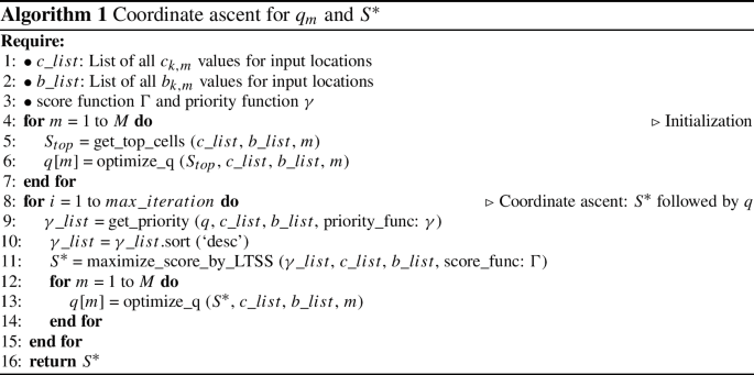
Finally, as the region $S^*$ detected by LTSS in Algorithm 1 may not be necessarily spatially contiguous (i.e., locations that are consecutive by priority $\gamma$ may not be spatially adjacent), we refine the partition with extra spatial smoothing (the localized scan in [20] does not work for our purpose as it tends to limit partitions to small and localized footprints). Specifically, at the final iteration of Algorithm 1, connected components in $S^*$ (i.e., subsets of grid cells) with a size that are smaller than a tolerance (defaulted to 3 cells) are swapped to the other partition $S'=S^i_j{\setminus } S^*$ where $S^i_j$ is the entire space at node ${\mathcal {H}}^i_j$. Similarly, for $S'$, we do the same swap of tiny components.

3.3.4 Complexity analysis

Here we provide the time complexity for Algorithm 1 at a ${\mathcal {H}}$-node. Denote n as the total number of samples and grid cells at the node, m as the number of classes, and t as the number of iterations (e.g., 1000). The complexity is then $O(t\cdot (n\log n + n + mn))$ (the cost of initialization and contiguity refinement is minimal and skipped here). Here the number of classes can be often considered as a constant, so the complexity reduces to $O(t\cdot n\log n)$. As described in Phase-3 of DL-MSS (Sect. 3.3.2), the number of cells of the grid is often very small at each node (e.g., 10 s to 100 s). Overall, we noticed that the total time spent on $S^*$ optimization is mostly negligible compared to the training time of network parameters in our experiments (e.g., second/minute vs. hour).

3.3.5 Regression version of DL-MSS

For regression, the general flow remains the same and the major differences are for the score function $\Gamma (S)$ and priority function $\gamma (s_k)$, which are needed as the prediction changes from multi-class labels to continuous values.

In this paper we focus on the scenario where each sample has one target label, i.e., $\textbf{y}\in {\mathbb {R}}^{N\times 1}$, where N is the number of samples. Also, instead of classification errors, we use mean squared errors $e_{k}$ for regression. For the score function $\Gamma (S)$, we select the normal-based likelihood ratio [23] (Poisson is used for classification), where the null hypothesis $H_0$ states that $e_k\sim \text {Normal}(\mu _{\text {all}}, \sigma ^2_{\text {all}})$ at all locations and $H_1$ states that there exists a region S where $e_k\in S \sim$ Normal($\mu _{S}, \sigma ^2_{\text {both}}$), and $e_k\in S' \sim$ Normal($\mu _{S'}, \sigma ^2_{\text {both}}$) for all other locations $S'$ (a common variance $\sigma ^2_{\text {both}}$ is used for both). To avoid redundancy, the simplified $\Gamma (S)$ and $S^*$ are (e.g., used by [23]):

$$\begin{aligned} \Gamma (S)= & {} N\ln {\frac{\sigma _{\text {all}}}{\sigma _{\text {both}}}} - \frac{N}{2} + \sum _{s_k\in S\cup S'}\frac{(e_k-\mu _{\text {all}})^2}{2\sigma _{\text {all}}^2} \end{aligned}$$

(7)

$$\begin{aligned} S^*= & {} \mathop {{{\,\mathrm{arg\,max}\,}}}\limits _S \Gamma (S) = \mathop {{{\,\mathrm{arg\,min}\,}}}\limits _S \sigma _{\text {both}} \end{aligned}$$

(8)

where only $N\ln {\sigma _{\text {both}}^{-1}}$ in $\Gamma (S)$ depends on S so maximizing $\Gamma (S)$ is equivalent to minimizing $\sigma _{\text {both}}$ or the variance $\sigma ^2_{\text {both}}$.

Based on Eq. (7), we have the following lemma:

Lemma 1

For $\Gamma (S)$ given in Eq. (7), the following priority function satisfies the LTSS property:

$$\begin{aligned} \gamma (s_k) = e_k \end{aligned}$$

(9)

Proof

The set of $\{e_k\}$ for locations $\{s_k\}$ is equivalent to a set of points distributed on a one-dimensional line. Moreover, the maximum likelihood estimators for the means and variances are $\mu _S = \vert S\vert ^{-1}\sum _{s_k\in S}e_k$, $\mu _{S'}=\vert S'\vert ^{-1}\sum _{s_k\in S'}e_k$, and $\sigma ^2_{\text {both}} = N^{-1}(\sum _{s_k\in S} (e_k-\mu _S)^2 + \sum _{s_k\in S'} (e_k-\mu _{S'})^2)$. Thus, minimizing the variance $\sigma ^2_{\text {both}}$ (or $\sigma _{\text {both}}>0$) is equivalent to minimizing the k-means loss with $k=2$. So for the two groups to be optimal, there should be no overlap in their $e_k$ value ranges on the 1D space, i.e., $\min _{s_k\in S}e_k \ge \max _{s_k\in S'}e_k$ assuming $\mu _S \ge \mu _{S'}$ (proof is symmetric for the other direction). Otherwise, swapping the minimum $e_k\in S$ and maximum $e_k\in S'$ must reduce the k-means loss (i.e., $N\sigma ^2_{\text {both}}$), either by center assignments or re-estimation. $\square$

3.4 A spatial moderator for generalization

The spatial hierarchy ${\mathcal {H}}$ and “spatialized” deep network ${\mathcal {F}}_{{\text {spatial}}}$ learned and trained from the transformation step aim to capture spatial heterogeneity for the spatial extent of the input $\textbf{X}$ and $\textbf{y}$. However, the partitions cannot be directly applied to a new spatial region. To bridge this gap, we propose a spatial moderator,¹ which translates the learned network branches in ${\mathcal {F}}_{{\text {spatial}}}$ to prediction tasks in a new region.

The key idea of the spatial moderator is to learn and predict a weight matrix $\textbf{W}$ for all branches in ${\mathcal {F}}_{{\text {spatial}}}$ (corresponding to all leaf-nodes in the spatial hierarchy ${\mathcal {H}}$), and then use the weights to ensemble the prediction results from the branches to get the final result. As an example, suppose the output ${\hat{\textbf{y}}}_i$ for a sample $\textbf{x}_i$ is in 1D. Then, in the weight matrix $\textbf{W}\in {\mathbb {R}}^{L\times M}$, the L rows each corresponds to a network branch in ${\mathcal {F}}_{{\text {spatial}}}$ (or a leaf node in ${\mathcal {H}}$), where the M columns correspond to the M labels (one-hot encoding for classification; $M=1$ for regression in this paper). Thus, every column in $\textbf{W}$ is a weight vector $\textbf{w}\in {\mathbb {R}}^{L}$ that gives the weight distribution across the branches for each of the M labels.

Fig. 3

Illustrative example of the spatial moderator

In the spatial moderator, $\textbf{W}$ is not stationary but predicted dynamically using each input data sample $\textbf{x}_i$. Fig. 3 shows the general architecture of the moderator. The left side shows an example of “spatialized” network ${\mathcal {F}}_{{\text {spatial}}}$ and the right side shows the corresponding spatial moderator. For a given sample $\textbf{x}_i$, the original ${\mathcal {F}}_{{\text {spatial}}}$ only generates predictions for the branch that $\textbf{x}_i$ spatially belongs to, i.e., ${\hat{\textbf{y}}}_i\in {\mathbb {R}}^M$. In this moderated version, ${\mathcal {F}}_{{\text {spatial}}}$ will generate predictions from all L branches for a sample $\textbf{x}_i$, i.e., ${\hat{\textbf{y}}}_i\in {\mathbb {R}}^{L\times M}$. Then, the moderator predicts the weight matrix $\textbf{W}\in {\mathbb {R}}^{L\times M}$ using the same sample $\textbf{x}_i$, and the final moderated prediction is:

$$\begin{aligned} {\hat{\textbf{y}}}_{\text {mod},i} = \text {softmax}(\textbf{1}^T ({\hat{\textbf{y}}}_i \odot \textbf{W})) \end{aligned}$$

(10)

where $\textbf{1}\in {\mathbb {R}}^L$ is a vector of ones [1,1...,1], and $\odot$ is element-wise (or Hadarmad) product.

The layer structure of the moderator we use here is a network with four densely connected layers with ReLU activations. If input $\textbf{x}_i$ is a time-series rather than a snapshot of features, the final layer is replaced with a LSTM layer (i.e., the first three layers are used to construct new features from the original input features, regardless of the timestamps, and the temporal patterns are learned through the final LSTM layer [24]). During the training of the moderator, all parameters from ${\mathcal {F}}_{{\text {spatial}}}$ will be frozen, and the moderator only needs to learn the weights for itself (the right side of Fig. 3).

4 STAR with meta-learning

The spatial transformation and moderation (STAR) framework spatializes an input deep network ${\mathcal {F}}$ using the automatically learned spatial hierarchy ${\mathcal {H}}$. This can be considered as exploration phase during which the model does not yet have the knowledge of, and is trying to figure out, the set $S_\Phi$ of different processes (or data generation functions) $\Phi : \textbf{X}\rightarrow \textbf{y}$ existing in the data. Thus, $S_\Phi$ is not determined until full completion of this phase (i.e., when ${\mathcal {H}}$ is completed). In a transfer learning context, this means the set of tasks $S_{\mathcal {T}}$ in the space is unknown, where each task corresponds to a process in $S_\Phi$. As a result, meta-learning-based enhancements, which can learn common knowledge from multiple known tasks and enable fast adaptation in limited data scenarios, cannot be leveraged during the exploration phase. On the other hand, such enhancements can be largely beneficial due to the following reasons: (1) As the spatial transformation process dives deeper into the spatial hierarchy ${\mathcal {H}}$ to distinguish heterogeneous processes, the spatial coverage of each node or partition becomes smaller. As a consequence, the amount of training data quickly reduces; and (2) The spatial moderator may often be needed in spatial regions where data samples available for fine-tuning are limited.

Thus, in this section, we present a meta-phase that executes after the spatial hierarchy ${\mathcal {H}}$ is learned by the exploration phase to integrate meta-learning into both the spatial transformation and moderation processes to improve knowledge-sharing and adaptation with limited samples.

4.1 Meta-learning for spatial transformation

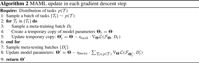
As the STAR framework is designed for general input network architectures ${\mathcal {F}}$, we maintain the flexibility of the meta-learning-enabled STAR (meta-STAR) using the model-agnostic meta-learning (MAML). As its name suggests, MAML is a general gradient descent framework that does not assume specific deep network architectures [25]. In the following, we first briefly demonstrate the basic concepts of MAML and its update rules.

The goal of MAML is to learn common knowledge from a distribution of tasks $p({\mathcal {T}})$, such that the trained model can be quickly adapted to a new task with limited training samples. To achieve this, each gradient descent step in MAML simulates this application scenario by the following:

• Create copies of the original model parameters $\theta$ and update each to $\varvec{\Theta }'_t$ using a mini-batch $D_t$—a batch with limited data samples—from a randomly sampled task ${\mathcal {T}}_t$ in $p({\mathcal {T}})$ (Eq. 11). This creates a set of models learned from existing tasks.

  $$\begin{aligned} \varvec{\Theta }'_t = \varvec{\Theta }- \eta _{\text {task}}\cdot \nabla _{\varvec{\Theta }}{\mathcal {L}}({\mathcal {F}}_{\varvec{\Theta }}, D_t) \end{aligned}$$

  (11)

  where $\eta _{\text {task}}$ is the learning rate.

• Next, to measure the effects of the updated parameters in $\{\varvec{\Theta }'_t\}$ to the performance of a new mini-batch $D'_t$ from task ${\mathcal {T}}_t$, MAML evaluates the losses of $\{\varvec{\Theta }'_t\}$ on $D'_t$ and computes the gradients (i.e., second-order derivatives with respect to the original model parameters $\varvec{\Theta }$). The gradients are then propagated back to $\varvec{\Theta }$ using:

  $$\begin{aligned} \begin{aligned} \varvec{\Theta }'&= \varvec{\Theta }- \eta _{\text {meta}}\cdot \sum _{{\mathcal {T}}_t\in p({\mathcal {T}})} \nabla _{\varvec{\Theta }}{\mathcal {L}}({\mathcal {F}}_{\varvec{\Theta }'_t}, D'_t)\\&= \varvec{\Theta }- \eta _{\text {meta}}\cdot \sum _{{\mathcal {T}}_t\in p({\mathcal {T}})} \nabla _{\varvec{\Theta }}{\mathcal {L}}({\mathcal {F}}_{ \varvec{\Theta }- \eta _{\text {task}}\cdot \nabla _{\varvec{\Theta }}{\mathcal {L}}({\mathcal {F}}_{\varvec{\Theta }}, D_t) }, D'_t) \end{aligned} \end{aligned}$$

  (12)

  where $\eta _{\text {meta}}$ is the learning rate for the meta-update. The meta-update rule of each gradient descent step in MAML is summarized in Algorithm 2.

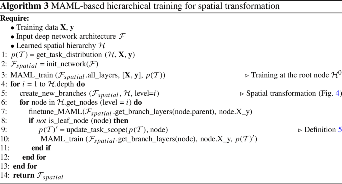
Next, we discuss the integration of MAML in the hierarchical spatial transformation process. Upon completion of transformation (Sect. 3.3.2), the set of tasks $S_{\mathcal {T}}$ for MAML can be determined by the leaf-nodes in ${\mathcal {H}}$, i.e., spatial partitions in which the process $\Phi$ is homogeneous. The probability distribution $p({\mathcal {T}})$ over the tasks can be calculated as $p({\mathcal {T}}_t) = \vert {\mathcal {T}}_t\vert /\sum _{{\mathcal {T}}_i} \vert {\mathcal {T}}_i\vert$, where $\vert {\mathcal {T}}_i\vert$ is the number of data samples in task ${\mathcal {T}}_i$; note that the distribution can also be estimated by users using other approaches or additional auxiliary information.

As the spatially transformed input network architecture ${\mathcal {F}}_{{\text {spatial}}}$ follows the hierarchical structure from ${\mathcal {H}}$ (Fig. 1), we integrate MAML into the training process following the same spatial hierarchy. Specifically, we restart the training following the same steps from the spatial transformation phase, except that we no longer need to perform the DL-MSS-based partitioning-optimization and significance testing, which can already been determined by ${\mathcal {H}}$. In addition, since we already know the task distribution at this point, MAML-based updates will be used (Algorithm 2) instead of the traditional gradient descent.

Given that the number of tasks available at a node in ${\mathcal {H}}$ gradually decreases as we propagate deeper into the hierarchy, the set of tasks to include for MAML update is scoped dynamically based on the following scope:

Definition 5

The scope of tasks at each node ${\mathcal {H}}^i_j\in {\mathcal {H}}$ includes all the leaf-nodes in ${\mathcal {H}}$ that are the children of ${\mathcal {H}}^i_j$.

Fig. 4 illustrates the MAML training process using examples at several nodes in ${\mathcal {H}}$. The spatial hierarchy used is the same as the example from Fig. 1, where there are four distinct tasks captured by the spatial transformation, as indicated by the four colors. The MAML training starts with all the tasks at the root node of ${\mathcal {H}}$, and gradually narrows the scope to subsets of tasks as the training proceeds to finer nodes.

Fig. 4

Example steps during hierarchical MAML training

Finally, we discuss the fine-tuning strategy used to dynamically re-condition the meta-learned parameters (or “common knowledge”) as the training moves deeper into the hierarchy. As the main purpose of MAML is to learn an initial set of weights among a set of tasks that can be quickly adapted or fine-tuned to new tasks, the adaptation needs to happen to fully harvest the enhancements. Thus, each time the training stage moves to a child node (e.g., from ${\mathcal {H}}^0$ to ${\mathcal {H}}^1_1$ in Fig. 4), we will first fine-tune the weights inherited from the parent node that are still fresh MAML-initializations, using the new tasks in the scope of the child node (Definition 5). Then, we switch back to MAML to meta-update the weights in the corresponding layers of the new branches (e.g., layers in the two gray-rectangles in Fig. 4b) based on the new tasks. If the child node is a leaf node (e.g., Fig. 4c, d), then we only perform the fine-tune step for the remaining single task. The process is illustrated in Algorithm 3.

4.2 Meta-learning for spatial moderation

The MAML training process for the spatial moderator is more straightforward, as all the parameters in moderator are shared by all data samples. Thus, for the moderator, we just need to use the full task distribution $p({\mathcal {T}})$ from ${\mathcal {H}}$ to perform MAML updates in each step according to Algorithm 2 (instead of using Algorithm 3, which is needed for spatial transformation to handle hierarchical updates). Note that here the MAML learned meta-weights will only be used for adaptation or finetuning with data from a new spatial region, and will no longer be finetuned for each task in $p({\mathcal {T}})$ from the original region. The reason is by design the moderator is for scenarios where the locations of samples are not inside the spatial coverage of the training data. As a result, location information should not used to determine which branch, or which set of parameters, to use during the prediction; otherwise, the moderator is not applicable to a new area and lost its original purpose. Thus, when the moderator is applied to samples inside the spatial coverage of the training data, we just train one set of parameters using all data (MAML will not be helpful in this case). In comparison, when limited labeled samples are available from a new region, we use MAML to train a meta-moderator with training data from the original region, and then adapt it to the new area.

5 Experiments

5.1 Real-world datasets

5.1.1 California land-cover classification

We use multi-spectral data from Sentinel-2 satellites in two regions in Central Valley, California. The first region ${\mathcal {D}}_{\text {ori}}$ has a size of 8192 $\times$ 4096 ($\sim$ 13422 km$^2$ in 20 m resolution), and the second ${\mathcal {D}}_{\text {new}}$ has a size of 4096 $\times$ 4096. The regions contain a wide variety of crops with strong heterogeneous patterns, resulting in a challenging classification task. The classes of ${\mathcal {D}}_{\text {ori}}$ and ${\mathcal {D}}_{\text {new}}$ are listed in Tables 1, 2, 3 and 4. Note that several land cover types have very low number of samples in region ${\mathcal {D}}_{\text {new}}$ (i.e., smaller than 0.025%), which are excluded from the table (no impact on the ranking of methods). We first learn the spatial partitioning using the data from region ${\mathcal {D}}_{\text {ori}}$ and then use the moderator to transfer it to ${\mathcal {D}}_{\text {new}}$. We use composite image series from May to October in 2018 (2 images/month) for time-series models, and one snapshot from August, 2018 for DNN. The labels are from the USDA Crop Data Layer (CDL) [26]. The training (and validation) set has 5% data at sampled locations in ${\mathcal {D}}_{\text {ori}}$, and 5% data in ${\mathcal {D}}_{\text {new}}$ is used for fine-tuning. The rest is used for testing.

5.1.2 Boston COVID-19 human mobility prediction

Human mobility provides critical information to COVID-19 transmission dynamics models. We acquired the Boston COVID-19 mobility dataset shared by [3], which includes data from US census, CDC COVID statistics, and SafeGraph patterns data. In this dataset, human mobility $\textbf{y}$ is represented by the number of visits to points-of-interest (POIs; e.g., grocery stores, restaurants) and the counting is based smartphone trajectories. We keep the same features $\textbf{X}$ used in [3], including population, weekly COVID-19 cases and deaths, number of POIs, week ID and income. The spatial representation of the data is a grid-partitioning (37 $\times$ 48) of the Boston area, and each cell is a data sample. Note that grid cells here are used to model the input data (similar to pixels in the California land-cover data), and is independent from the grid G we used in our partition-optimization approach (Sect. 3.3.2). The dataset contains 12 weeks of data, and according to [3], we use the first 11 weeks for training/validation and the final week for testing.

5.2 Base models ${\mathcal {F}}$, Implementation and Training

We implemented the spatial transformation and moderation framework for both snapshot- and time-series-based network models. Specifically, for snapshot models, we use densely connected network (DNN) to learn from data labels sampled at a subset of locations (commonly used in real-world field surveys for ground-truth collection). For time-series models, we use LSTM that was a common architecture choice for land-cover mapping with a sequence of satellite imagery [24, 27]. All the models have 7 hidden layers, each with 10 neurons and a ReLU activation, to learn and construct new features from raw inputs. For LSTM, an extra LSTM layer is added at the end to learn temporal patterns. A softmax layer is used for the output layer in classification.

Both DNN and LSTM are used as base network architectures ${\mathcal {F}}$. We obtain the learned spatial hierarchy ${\mathcal {H}}$ and synchronized architecture ${\mathcal {F}}_{\mathcal {H}}$ (same as ${\mathcal {F}}_{{\text {spatial}}}$; used to save space in result tables). As here DNN and LSTM share the same static feature processing architecture, we train DNN first and use the DNN weights to initialize LSTM training. Two versions of ${\mathcal {F}}_{\mathcal {H}}$ are used in comparison, where one is trained with MAML (Sect. 4.1) and the other trained with regular gradient descent (i.e., regular updates instead of MAML updates). Similarly, spatial moderators are also implemented in two forms, i.e., MAML-based and non-MAML-based versions. For training, we use the Adam optimizer with initial learning rate set to 0.01. All the model parameters in ${\mathcal {F}}$ and ${\mathcal {F}}_{\mathcal {H}}$ (regardless of branches) are trained with 600 epochs. All the models, when fine-tuned (e.g., for region ${\mathcal {D}}_{\text {new}}$ in California data), are allocated with an extra 200 epochs. For candidate methods with spatial moderator, only moderator weights are fine-tuned. The loss functions for classification and regression are cross-entropy and mean-squared errors, respectively. Code is available at: https://github.com/yqthanks/STAR.

5.3 Candidate methods

For California land-cover classification, we have the following candidate methods for each base model (i.e., DNN or LSTM): (1) Base model ${\mathcal {F}}$ itself; (2) Four versions of clustering-enhanced models. The goal of additional clustering is to create better baselines that use data partitioning to learn different functions for different clusters. Here the data samples are clustered based on their feature similarity, and a model is learned for each cluster by finetuning ${\mathcal {F}}$ with the cluster’s contained data subset. We consider two clustering algorithms: K-means++ and Deep Embedding Clustering (DEC) [28], each with two different numbers of clusters 10 and 20. We denote the models as: ${\mathcal {F}}^{10}_{\text {km}}$, ${\mathcal {F}}^{20}_{\text {km}}$, ${\mathcal {F}}^{10}_{\text {dec}}$, and ${\mathcal {F}}^{20}_{\text {dec}}$, respectively. (3) Two versions of spatially transformed ${\mathcal {F}}$: ${\mathcal {F}}_{\mathcal {H}}$ without MAML and ${\mathcal {F}}^{\text {meta}}_{\mathcal {H}}$ with MAML; and (4) Two versions of moderator: ${\mathcal {F}}_M$ without MAML and ${\mathcal {F}}^{\text {meta}}_M$ with MAML. As described in Sect. 4.2, ${\mathcal {F}}^{\text {meta}}_M$ is only needed for prediction in the new region ${\mathcal {D}}_{\text {new}}$. The two versions of the spatial moderator are trained using the same spatially transformed model (i.e., ${\mathcal {F}}_{\mathcal {H}}$ or ${\mathcal {F}}^{\text {meta}}_{\mathcal {H}}$) for direct comparison; we choose ${\mathcal {F}}^{\text {meta}}_{\mathcal {H}}$ in experiments as it has a better performance.

For Boston COVID-19 human mobility regression, we have the following candidate methods for comparison: the geographically weighted regression (GWR), which is a traditional linear inference model with consideration of spatial heterogeneity; base deep learning model (DNN) ${\mathcal {F}}$; clustering-enhanced models ${\mathcal {F}}^{10}_{\text {km}}$, ${\mathcal {F}}^{20}_{\text {km}}$, ${\mathcal {F}}^{10}_{\text {dec}}$ and ${\mathcal {F}}^{20}_{\text {dec}}$; spatially transformed ${\mathcal {F}}_{\mathcal {H}}$ (without MAML) and ${\mathcal {F}}^{\text {meta}}_{\mathcal {H}}$ (with MAML). As this dataset contains one single spatial region for different timestamps (Sect. 5.1), the space-partitioning learned during training can be directly applied on the test samples, which is the same as the scenario in ${\mathcal {D}}_{\text {ori}}$ for land cover classification. Thus, here we use ${\mathcal {F}}_{\mathcal {H}}$ and ${\mathcal {F}}^{\text {meta}}_{\mathcal {H}}$ instead of ${\mathcal {F}}_M$ and ${\mathcal {F}}^{\text {meta}}_M$.

Table 1 Region ${\mathcal {D}}_{\text {ori}}$: F1-scores of land-cover classification using sentinel-2 multi-spectral imagery (snapshot)

Table 2 Region ${\mathcal {D}}_{\text {ori}}$: F1-scores of land-cover classification using sentinel-2 multi-spectral imagery (time-series)

5.4 Results

5.4.1 Land-cover classification

Tables 1, 2, 3 and 4 show the F1-scores of the 10 candidate methods for the two spatial regions ${\mathcal {D}}_{\text {ori}}$ (5% for training and 5% for validation) and ${\mathcal {D}}_{\text {new}}$ (5% of data for fine-tuning), respectively. Both class-wise F1 scores and the overall weighted average are included in the tables. For the STAR and meta-STAR (Sect. 5.3), the spatial hierarchy are learned with training data in region ${\mathcal {D}}_{\text {ori}}$. Then, in region ${\mathcal {D}}_{\text {new}}$, the learned weights in ${\mathcal {F}}_{\mathcal {H}}$ and ${\mathcal {F}}^{\text {meta}}_{\mathcal {H}}$ are kept frozen and only each corresponding moderator is finetuned with the 5% samples. This helps evaluate if the heterogeneous spatial processes $\{\Phi \}$ learned in ${\mathcal {D}}_{\text {ori}}$ can be generalized to the new region ${\mathcal {D}}_{\text {new}}$ with the moderator, which re-mixes the processes $\{\Phi \}$ based on characteristics of test data samples.

The general trend is that the “spatialized” network architectures overall achieved better F1-scores for both snapshot- and time-series-based models in both regions. Moreover, the integration of MAML-based hierarchical training strategies further improved the performances and achieved the highest F1 scores. The performance differences in region ${\mathcal {D}}_{\text {new}}$ are smaller as forests and grasslands cover the majority of the landscape in this new region, making the classification problem relatively easier. The performance improvement achieved by the clustering-enhanced models were not very stable. For example, they all led to improvements over the base model ${\mathcal {F}}$ in Table 2, but had similar or reduced scores compared to ${\mathcal {F}}$ in the other scenarios. This is potentially because clustering does not consider the functional relationships $\textbf{X}\rightarrow \textbf{y}$ between $\textbf{X}$ and $\textbf{y}$. As a result, data samples within a cluster can still have different distributions and those from different clusters may have the same distribution, making the learning not as effective. The performances were similar between models based on K-means and DEC, and between 10 and 20 clusters. We also tested out other numbers of clusters (e.g., 5) and other clustering methods such as spectral clustering and hierarchical density-based clustering (HDBSCAN) [29], which did not perform as well, so we used the current four versions in the tables.

Table 3 Region ${\mathcal {D}}_{\text {new}}$: F1-scores of land-cover classification using sentinel-2 multi-spectral imagery (snapshot)

Table 4 Region ${\mathcal {D}}_{\text {new}}$: F1-scores of land-cover classification using sentinel-2 multi-spectral imagery (time-series)

Fig. 5

The decreases of loss values during spatial transformation for ${\mathcal {F}}_{\mathcal {H}}$ (dashed-lines) and ${\mathcal {F}}^{\text {meta}}_{\mathcal {H}}$ (solid lines)

Fig. 6

The increases of F1-scores on test data during spatial transformation for ${\mathcal {F}}_{\mathcal {H}}$ (dashed-lines) and ${\mathcal {F}}^{\text {meta}}_{\mathcal {H}}$ (solid lines)

We additionally included Fig. 5 and 6 to better visualize the performance improvements by the spatial-heterogeneity-awareness and meta-learning. Figure 5 shows the decreases of loss values for both ${\mathcal {F}}_{\mathcal {H}}$ and ${\mathcal {F}}^{\text {meta}}_{\mathcal {H}}$ in each node (or partition) as the spatial transformation process proceeds to separate out heterogeneous processes $\Phi$. This illustrative graph is generated using DNN as the base model. In the tuning columns in Fig. 5, the solid lines show the decrease from the MAML-based ${\mathcal {F}}^{\text {meta}}_{\mathcal {H}}$ and the dash line represent traditional gradient based updates in ${\mathcal {F}}_{\mathcal {H}}$. To reduce the crowdedness in Fig. 5 (e.g., the last column), we used binary-encoding to mark different nodes. For example, “0” and “1” refer to the two level-1 nodes in ${\mathcal {H}}$ after the first split (i.e., ${\mathcal {H}}^1_1$ and ${\mathcal {H}}^1_2$, and ”01” means child-“1” in level-2 of node “0” in level-1. We can see that the MAML-based ${\mathcal {F}}^{\text {meta}}_{\mathcal {H}}$ reaches better performances as the amounts of training samples decrease as the model dives deeper into the hierarchy. Furthermore, combined together with the F1-score results in Fig. 6, which shows the F1-scores on test data samples (aggregated from all the local nodes at each level), we can see that the overall F1-scores of both ${\mathcal {F}}^{\text {meta}}_{\mathcal {H}}$ and ${\mathcal {F}}_{\mathcal {H}}$ improve as spatial heterogeneity are captured through the spatial transformation process.

For region ${\mathcal {D}}_{\text {ori}}$, the results ${\mathcal {F}}$, ${\mathcal {F}}_{\mathcal {H}}$ and ${\mathcal {F}}^{\text {meta}}_{\mathcal {H}}$ for each base model can be used for ablation analysis. The general trend is that the results of a base model ${\mathcal {F}}$ gradually improve with the addition of spatial transformation ${\mathcal {F}}_{\mathcal {H}}$, and the MAML-based meta learning ${\mathcal {F}}^{\text {meta}}_{\mathcal {H}}$.

In addition, Fig. 7 shows the hierarchical process of space-partitioning with DL-MSS (Sect. 3.3.2) for the first two levels. In the first level (largest scale), for example, ${\mathcal {H}}^1_1$ is a mix of urban and suburban areas, whereas ${\mathcal {H}}^1_2$ contains more rural and mountainous areas. Note that some partitions (e.g., ${\mathcal {H}}^2_3$) are not further split, as determined by significance testing. Also, a partition is allowed to contain multiple disconnected areas as long as they satisfy the minimum footprint size enforced for contiguity (Sect. 3.3.3). Nonetheless, we can see the automatically captured footprints are in general spatially contiguous as a result of spatial auto-correlation. Finally, Fig. 8 visualizes the weights predicted by the moderator for two example network branches in ${\mathcal {F}}^{\text {meta}}_{\mathcal {H}}$ for DNN (paths from input to output layers; Fig. 3) for all locations in region ${\mathcal {D}}_{\text {new}}$. For each branch, the weight is averaged over all classes in the predicted $\textbf{W}$ at each location. As we can see, in the new region ${\mathcal {D}}_{\text {new}}$, branch-17 is given higher weights for the left-side of the region, which is a mountainous area. Branch-6 receives higher weights in the top-left corner, which contains large flat farmlands. In contrast, branch-4 is not assigned high weights by nearly all locations in ${\mathcal {D}}_{\text {new}}$. In the original region ${\mathcal {D}}_{\text {ori}}$, this branch represents large flat barren lands, which has limited appearance in ${\mathcal {D}}_{\text {new}}$.

Fig. 7

Spatial hierarchy learned in region ${\mathcal {D}}_{\text {ori}}$ (the first two levels)

Fig. 8

Learned branch weights across space (across samples)

5.4.2 COVID-19 mobility regression

Table 5 shows the results of the five candidate methods, where we used three measures for the evaluation: mean absolute errors (MAE), root mean squared errors (RMSE), and symmetric mean absolute percentage error (sMAPE). We used sMAPE instead of MAPE because there are many locations—especially during the COVID-19 scenario—with very few or zero POI visits. This makes the results of MAPE frequently undefined (e.g., positive number divided by zero) for the candidate methods. In contrast, sMAPE addresses this issue by including the predicted values in the denominator for percentage calculation. We used the version of sMAPE that has a range from 0 to 100%. The values for sMAPE are relatively high for all methods, and this is mainly caused by many locations with very small numbers of POI visits. Fig 9 shows maps of the ground truth, GWR, ${\mathcal {F}}$ (DNN), ${\mathcal {F}}_{{{\mathcal {H}}}}$ and ${\mathcal {F}}^{\text {meta}}_{{{\mathcal {H}}}}$. Several potential causes of spatial heterogeneity here include different mobility patterns in the more populous downtown area versus the suburban regions, and several “hotspot” areas of POI visits that are a bit abnormal compared to the rest.

As we can see, overall ${\mathcal {F}}_{{{\mathcal {H}}}}$ and ${\mathcal {F}}^{\text {meta}}_{{{\mathcal {H}}}}$ achieved better results for the three measures, and ${\mathcal {F}}^{\text {meta}}_{{{\mathcal {H}}}}$ obtained further improvements with meta-learning. The improvements are relatively smaller (e.g., RMSE) compared to the California land cover classification task, which is potentially due to the smaller number of tasks. Although GWR performs spatially localized regression, it can only handle linear relationships using input variables and apply the same spatial neighborhood for all locations, which cannot well capture non-stationary mobility hotspots and variation in the data. Moreover, the data-reduction problem caused by local-regression in GWR frequently causes existing standard libraries to run into ill-conditioned problems if small band-widths are used. Three out of the four clustering-enhanced models achieved improvements over the base model ${\mathcal {F}}$, but the improvements were limited potentially due to the lack of consideration on the functional relationships between $\textbf{X}$ and $\textbf{y}$. Similarly, we tested out other numbers of clusters (e.g., 5) and clustering methods, which did not provide better results. Finally, the spatial transformation automatically identified three heterogeneous partitions (other splits are statistically insignificant) and branched out downtown, suburban and several mobility hotspots (our method allows large footprints at multiple locations to be in one node), greatly improving the performance on both types of measures.

Table 5 COVID-19 human mobility projection

Fig. 9

Visualization of human mobility maps

6 Other related work

Existing methods for handling heterogeneity can be generally divided into two categories. The first class aims to transfer parameters learned from one source to another, such as domain adaptation [30,31,32] and meta-learning (e.g., MAML) [25, 33, 34]. However, these methods mainly focus on the learning of robust features and fast adaptation, and may yield degraded performance when spatial regions have large discrepancy. Moreover, they require a pre-defined space-partitioning of heterogeneous processes. It is worth-mentioning though that these methods and the proposed STAR framework are complementary and can be integrated for further enhancements. For example, meta-learning has been incorporated into the STAR framework as shown in Sect. 4. The second direction is based on explicit data partitioning. For example, researchers have separately trained individual local models for different data clusters [35, 36] and have shown improved performance against a single global model. However, the clustering only uses input features that are not sufficient to capture underlying heterogeneous processes. Similarly, local training has been used for manually defined spatial regions, e.g., ANN [10] and RNN [37]. Furthermore, all these methods can significantly reduce the training data available for local models, making it difficult to train complex models. Spatial-Net also uses the hierarchical multi-task representation for parameter sharing [18], but cannot handle irregular partitionings (i.e., spatial footprints with arbitrary shapes) or be generalized to new regions; it does guarantee each partition’s spatial contiguity. Finally, mixture process mining [38] can find regions where data are generated by homogeneous-mixture processes $\{\Phi \}$ but cannot handle deep learning inputs where $\{\Phi : \textbf{X}\rightarrow \textbf{y}\}$ are often unknown and cannot be directly defined by statistical models (e.g., Poisson).

7 Conclusions and future work

We proposed a model-agnostic meta-STAR framework for spatial data and problems, which is an extension of STAR in [16]. The STAR framework can: (1) simultaneously learn arbitrarily shaped space-partitionings of heterogeneous processes and a “spatialized” network architecture; and (2) generalize learned spatial structures to new regions. We extended the STAR framework with meta-learning (meta-STAR) to further improve knowledge sharing and adaptation. Experiments on real world datasets showed that the framework can substantially improve the performance of base networks on spatial problems, and that meta-learning can enhance knowledge adaptation.

In future work, we will explore the use of the framework on other types of network architectures such as GAN, CNN and GCN, and traditional machine learning methods. Furthermore, we plan to investigate specific characteristics of each type of network architecture in the context of spatial heterogeneity and identify dedicated customizations of the current framework. Finally, we will explore generalizations with other types of space-partitioning schemes, statistical formulations, etc.

References

Group on earth observations global agricultural monitoring initiative (2021). https://earthobservations.org/geoglam.php
Kraemer MU et al (2020) The effect of human mobility and control measures on the covid-19 epidemic in china. Science 368(6490):493–497
Bao H, Zhou X, Zhang Y, Li Y, Xie Y (2020) Covid-gan: estimating human mobility responses to covid-19 pandemic through spatio-temporal conditional generative adversarial networks. In: Proceedings of the 28th international conference on advances in geographic information systems, pp 273–282
Atluri G, Karpatne A, Kumar V (2018) Spatio-temporal data mining: a survey of problems and methods. ACM Comput Surv (CSUR) 51(4):1–41
Shekhar S, Feiner SK, Aref WG (2015) Spatial computing. Commun ACM 59(1):72–81
Goodchild MF, Li W (2021) Replication across space and time must be weak in the social and environmental sciences. Proc Natl Acad Sci 118(35):e2015759118
Karpatne A, Ebert-Uphoff I, Ravela S, Babaie HA, Kumar V (2018) Machine learning for the geosciences: challenges and opportunities. IEEE Trans Knowl Data Eng 31(8):1544–1554
Krizhevsky A, Sutskever I, Hinton GE (2012) Imagenet classification with deep convolutional neural networks. Adv Neural Inf Process Syst 25:1097–1105
He K, Zhang X, Ren S, Sun J (2016) Deep residual learning for image recognition. In: CVPR, pp 770–778
Gupta J et al (2020) Towards spatial variability aware deep neural networks (svann): a summary of results. In: ACM SIGKDD workshop on deep learning for spatiotemporal data, applications and systems
Gupta J et al (2021) Spatial variability aware deep neural networks (SVANN): a general approach. ACM Trans Intell Syst Technol. https://doi.org/10.1145/3466688
Jiang Z, Li Y, Shekhar S, Rampi L, Knight J (2017) Spatial ensemble learning for heterogeneous geographic data with class ambiguity: a summary of results. In: Proceedings of the 25th ACM SIGSPATIAL international conference on advances in geographic information systems, pp 1–10
Jiang Z et al (2019) Spatial ensemble learning for heterogeneous geographic data with class ambiguity. ACM Trans Intell Syst Technol 10(4):1–25
Brunsdon C, Fotheringham AS, Charlton M (1999) Some notes on parametric significance tests for geographically weighted regression. J Reg Sci 39(3):497–524
Fotheringham AS, Yang W, Kang W (2017) Multiscale geographically weighted regression (MGWR). Ann Am Assoc Geogr 107(6):1247–1265
Xie Y, He E, Jia X, Bao H, Zhou X, Ghosh R, Ravirathinam P (2021) A statistically-guided deep network transformation and moderation framework for data with spatial heterogeneity. In: IEEE international conference on data mining (ICDM)
Kratsios A, Bilokopytov I (2020) Non-euclidean universal approximation. NeurIPS 33:10635–10646
Xie Y, Jia X, Bao H, Zhou X, Yu J, Ghosh R, Ravirathinam P (2021) Spatial-net: a self-adaptive and model-agnostic deep learning framework for spatially heterogeneous datasets. In: Proceedings of the 29th international conference on advances in geographic information systems, pp 313–323
Kulldorff M, Mostashari F, Duczmal L, Katherine Yih W, Kleinman K, Platt R (2007) Multivariate scan statistics for disease surveillance. Stat Med 26(8):1824–1833
Neill DB, McFowland E III, Zheng H (2013) Fast subset scan for multivariate event detection. Stat Med 32(13):2185–2208
Xie Y, Shekhar S, Li Y (2022) Statistically-robust clustering techniques for mapping spatial hotspots: a survey. ACM Comput Surv (CSUR) 55(2):1–38
Neill DB (2012) Fast subset scan for spatial pattern detection. J Roy Stat Soc 74(2):337–360
Kulldorff M, Huang L, Konty K (2009) A scan statistic for continuous data based on the normal probability model. Int J Health Geogr 8(1):1–9
Jia X, Li S, Khandelwal A, Nayak G, Karpatne A, Kumar V (2019) Spatial context-aware networks for mining temporal discriminative period in land cover detection. In: SDM. SIAM, pp 513–521
Finn C, Abbeel P, Levine S (2017) Model-agnostic meta-learning for fast adaptation of deep networks. In: International conference on machine learning. PMLR, pp 1126–1135
USDA cropland data layer (2021). https://www.nass.usda.gov/Research_and_Science/Cropland/SARS1a.php
RuBwurm M, Körner M (2017) Temporal vegetation modelling using long short-term memory networks for crop identification from medium-resolution multi-spectral satellite images. In: CVPR workshops, pp 1496–1504
Xie J, Girshick R, Farhadi A (2016) Unsupervised deep embedding for clustering analysis. In: International conference on machine learning. PMLR, pp 478–487
Campello RJ, Moulavi D, Sander J (2013) Density-based clustering based on hierarchical density estimates. In: Pacific-asia conference on knowledge discovery and data mining. Springer, pp 160–172
Zhang Y, David P, Gong B (2017) Curriculum domain adaptation for semantic segmentation of urban scenes. In: Proceedings of the IEEE international conference on computer vision, pp 2020–2030
Jia X, Nayak G, Khandelwal A, Karpatne A, Kumar V (2019) Classifying heterogeneous sequential data by cyclic domain adaptation: an application in land cover detection. In: SDM. SIAM
Pei Z, Cao Z, Long M, Wang J (2018) Multi-adversarial domain adaptation. In: Thirty-second AAAI conference on artificial intelligence
Rußwurm M, Wang S, Korner M, Lobell D (2020) Meta-learning for few-shot land cover classification. In: Proceedings of the IEEE/CVF conference on computer vision and pattern recognition workshops, pp 200–201
Yao H, Liu Y, Wei Y, Tang X, Li Z (2019) Learning from multiple cities: a meta-learning approach for spatial-temporal prediction. In: The world wide web conference, pp 2181–2191
Karpatne A, Khandelwal A, Boriah S, Kumar V (2014) Predictive learning in the presence of heterogeneity and limited training data. In: SDM. SIAM, pp 253–261
Tarabalka Y, Benediktsson JA, Chanussot J (2009) Spectral-spatial classification of hyperspectral imagery based on partitional clustering techniques. IEEE Trans Geosci Remote Sens 47(8):2973–2987
Yuan Z, Zhou X, Yang T (2018) Hetero-convlstm: a deep learning approach to traffic accident prediction on heterogeneous spatio-temporal data. In: ACM SIGKDD, pp 984–992
Xie Y, Bao H, Li Y, Shekhar S (2020) Discovering spatial mixture patterns of interest. In: Proceedings of the 28th international conference on advances in geographic information systems, pp 608–617
Acknowledgements
This material is based upon work supported by the National Science Foundation under Grant Nos.2105133, 2126474 and 2147195; NASA under Grant Nos. 80NSSC22K1164 and 80NSSC21K0314; USGS under Grant No. G21AC10207; US-DOT under Grant No.69A3551747131 (through SAFER-SIM); Google’s AI for Social Good Impact Scholars program; the DRI award at the University of Maryland; Pitt Momentum Funds award and CRC at the University of Pittsburgh; and the ISSSF grant from the University of Iowa.
Author information
Authors and Affiliations
Corresponding author
Additional information
Publisher's Note
Springer Nature remains neutral with regard to jurisdictional claims in published maps and institutional affiliations.
Rights and permissions
Springer Nature or its licensor (e.g. a society or other partner) holds exclusive rights to this article under a publishing agreement with the author(s) or other rightsholder(s); author self-archiving of the accepted manuscript version of this article is solely governed by the terms of such publishing agreement and applicable law.
About this article
Cite this article
Xie, Y., Chen, W., He, E. et al. Harnessing heterogeneity in space with statistically guided meta-learning. Knowl Inf Syst 65, 2699–2729 (2023). https://doi.org/10.1007/s10115-023-01847-0
Received:
Revised:
Accepted:
Published:
Issue Date:
DOI: https://doi.org/10.1007/s10115-023-01847-0