Abstract
In this work, in the context of Linear and convex Quadratic Programming, we consider Primal Dual Regularized Interior Point Methods (PDR-IPMs) in the framework of the Proximal Point Method. The resulting Proximal Stabilized IPM (PS-IPM) is strongly supported by theoretical results concerning convergence and the rate of convergence, and can handle degenerate problems. Moreover, in the second part of this work, we analyse the interactions between the regularization parameters and the computational footprint of the linear algebra routines used to solve the Newton linear systems. In particular, when these systems are solved using an iterative Krylov method, we are able to show—using a new rearrangement of the Schur complement which exploits regularization—that general purposes preconditioners remain attractive for a series of subsequent IPM iterations. Indeed, if on the one hand a series of theoretical results underpin the fact that the approach here presented allows a better re-use of such computed preconditioners, on the other, we show experimentally that such (re)computations are needed only in a fraction of the total IPM iterations. The resulting regularized second order methods, for which low-frequency-update of the preconditioners are allowed, pave the path for an alternative class of second order methods characterized by reduced computational effort.
1 Introduction
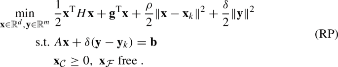
In this work we consider the problem of solving the following primal-dual convex quadratic programs:
where the dual problem has been obtained considering the Lagrangian function
and where \(H \in {\mathbb {R}}^{d \times d}\) with \(H \succeq 0\), \(A \in {\mathbb {R}}^{m \times d}\) with \(m \le d\) is not required to have full rank. We assume, moreover, for simplicity of exposition and w.l.g., that \({\mathcal {F}}=\{1,\dots ,\bar{d}\}\) and \({\mathcal {C}}=\{\bar{d}+1, \dots , d\}\) for some \(0 \le \bar{d} \le d\), and define \( {\mathcal {F}} = \emptyset \) if \(\bar{d} = 0\) or \( {\mathcal {C}} = \emptyset \) if \(\bar{d} = d\).
For the past few decades, Interior Point Methods (IPMs) [13, 31] have gained wide appreciation due to their remarkable success in solving linear and convex quadratic programming problems (1). The computational cost of an IPM iteration is dominated by the solution of a Karush–Kuhn–Tucker (KKT) linear system of the form
where the diagonal matrix \(\varTheta :={{{\,\textrm{diag}\,}}({\textbf{x}})^{-1}{{\,\textrm{diag}\,}}({\textbf{s}})}\) and the right hand side changes at every iteration. The diagonal correction \(\varTheta \) represents, somehow, the core of the IPM methodology and acts, essentially, as a continuous approximation of the indicator function for labelling active and non-active variables based on the magnitude of its diagonal elements: in the limit, these elements approach 0 or \(+\infty \).
A closer look at the KKT system in (3), reveals how the astonishing polynomial worst-case complexity of IPMs [13, 31] is counterbalanced by an intrinsic difficulty for the optimal tuning of the linear algebra solvers required for their implementation. We briefly summarize two such issues:
-
(I1)
near rank deficiency of A, or near singularity of \(H + {\varTheta ^{-1}}\), can give rise to inefficient or unstable solutions of the KKT linear systems. This may occur regardless of whether a direct or iterative method is used for their solution. Moreover, it is important to mention at this point the related issue concerning the fact that, in case of a rank deficiency of A, the theory of convergence for IPM is not clear.
-
(I2)
for large scale problems, the unwelcome feature displayed by the diagonal elements of \(\varTheta ^{-1}\) represents a paradigmatic example of how Krylov methods may be easily made ineffective due to the fact that the conditioning of the involved linear systems deteriorates as the IPM iterations proceed. As a result, the robustness and efficiency of IPMs depend heavily on the use of preconditioners which should be recomputed/updated at every iteration due to the presence of the rapidly changing matrix \(\varTheta ^{-1}\).
1.1 Motivations and Background
In the last 20 years there has been an intense research activity regarding items (I1) and (I2) mentioned in the previous section. In particular, in order to alleviate some of the numerical difficulties related to (I1), it has been proposed in [2] to systematically modify the linear system (3) using, in essence, a diagonal regularization. Despite the fact that this strategy has proven to be effective in practice, to the best of our knowledge, in literature few works are devoted to the complete theoretical understanding of these regularization techniques. We mention [11], where the global convergence of an exact primal-dual regularized IPM is shown under the somehow strong hypothesis that the computed Newton directions are uniformly bounded (see [11, Th. 5.4]) and [25], where regularization is interpreted in connection with the Augmented Lagrangian Method [17] and the Proximal Method of Multipliers [26] and where the convergence to the true solution is recovered when the regularization is driven to zero at a suitable speed.
Concerning (I2), the literature is quite extensive and it is not possible to give a short comprehensive outlook. We refer the interested reader to [13, Sec. 5] and [6] for a comprehensive survey. We prefer to stress, instead, the fact that the presence of the iteration dependent matrix \(\varTheta \) and its diverging elements represents, somehow, the true challenge in the efficient implementation of IPMs for large scale problems. As a matter of fact, the computational costs related to the necessary re-computations of factorizations and/or preconditioners for the Newton linear systems represent the main bottleneck of the existing implementations.
It is important to note, moreover, that when factorizations are used as back-solvers for Newton systems, the issue of reducing systematically the number of such necessary factorizations has been successfully addressed using the Multiple Centrality Corrections (MCC) strategy, see [5, 15]. Indeed, in this context, the use of a given factorization is maximized by applying it to solve several linear systems and producing modified Newton directions in which larger steps can be made, ultimately reducing the number of IPM iterations. On the other hand, when a very good preconditioner is not available, the use of Krylov iterative methods [30] for the solution of the Newton systems makes the MCC strategy consistently less appealing. At large, the results presented in this work aim at achieving the same goals as the MCC strategy, i.e., reducing the number of factorization re-computations, but when Krylov methods are used as back-solvers for the Newton systems and when a given factorization is used as preconditioner.
As it will be clear from our theoretical developments, the main tool used to solve/alleviate simultaneously the issues outlined in items (I1) and (I2) is the regularization. Indeed, broadly speaking, this work can be viewed as a study of the interactions between the regularization parameters used in the Primal Dual Regularized Interior Point Methods (PDR-IPMs) and the computational footprint of the linear algebra routines used to solve the related Newton linear systems.
1.2 Contribution and Organization
The investigation which aims at addressing both issues (I1) and (I2) is naturally organized into two main threads. Indeed, in the first part of this work we aim at clarifying how alleviating the (near) rank deficiency of matrix A using regularization affects the convergence of the underlying IPM scheme. To this end, we build a bridge between Primal Dual Regularized IPMs (PDR-IPMs) and the Proximal Point Method (PPM) [28] giving a precise description of the synergies occurring between them. In particular, our analysis contributes to the understanding of the hidden machinery which controls the convergence of the PDR-IPM and clarifies, finally, the influence of regularization for PDR-IPMs: our proposal, the Proximal Stabilized IPM (PS-IPM), is strongly supported by theoretical results concerning convergence/rate of convergence and can handle degenerate problems as those described in (I1).
In the second part of this work, building the momentum from the developed convergence theory, we address (I2) using a PS-IPM perspective. Here we prove that regularization can be used, in fact, as a tool to pursue the challenging aspiration of reducing systematically the number of necessary preconditioner re-computations needed for the iterative solution of IPM Newton linear systems. Indeed, using an equivalent formulation of the LP/QP problem and a new rearrangement of the Schur complements for the related Newton systems, when such systems are solved using an iterative Krylov method, we are able to prove a series of theoretical results showing that the computed preconditioners are re-usable during the IPM iterations. The presented numerical results further underpin this claim showing that the number of sufficient preconditioner re-computations equals just a fraction of the total IPM iterations when general purpose preconditioners are used. As a straightforward consequence of the above findings, we are able to devise a class of IPM-type methods characterized by the fact that the re-computation of any given preconditioner can be performed in low-frequency regime, hence the linear algebra footprint of the method is significantly reduced.
The precise outline of the contribution and the organization of the work can be summarized as follows.
In Sects. 2 and 3, using the PPM [28] in its inexact variant [20], we prove the convergence of the PDR-IPM-type schemes for the solution of problem (1) without any further assumptions on the uniform boundedness of the Newton directions or assuming that the regularization is driven to zero. Indeed, if on one hand our PS-IPM sheds further light on the experimental evidence that regularization is of extreme importance for robust and efficient IPMs implementations, on the other, it is supported by a precise result, see Theorem 2.1, tying the magnitude of the regularization parameters to its rate of convergence. The experimental evidence of the goodness of the proposed framework and of the resulting implementation is presented in Sect. 5.2 where we show that, when direct methods are used for the solution of the Newton system, fixing the regularization parameters to small values is preferable to a strategy in which a decreasing sequence of regularization parameters is employed.
In Sect. 4, we are able to depict a precise quantitative picture on the relations intervening between the regularization parameters and the necessity of recomputing any given preconditioner. Indeed, heavily relying on the form of the primal-dual regularized Newton systems and using a novel rearranging of their Schur complement which is based on a separation of variables trick, we propose and analyse a new preconditioning technique for which the frequency of re-computation depends inversely on the magnitude of the regularization parameters. As a result, in the proposed PS-IPM scheme, the overall computational footprint of the linear algebra solvers can be decreased at the cost of slowing down its rate of convergence.
Finally, in Sect. 5, we carry out an experimental analysis of PS-IPMs when the corresponding Newton systems are solved using a Krylov iterative method precoditioned as proposed in Sect. 4. The presented results show that the proposed algorithm can be tuned to obtain a number of preconditioner updates roughly equal to one third of the total IPM iterations while maintaining an IPM-type rate of convergence, leading, hence, to improvements of the computational performance in large scale settings.
1.3 Notation
In the following \({\textbf{x}},{\textbf{y}},{\textbf{z}},\dots \) are vectors and, given \(Q \in {\mathbb {R}}^{u \times u}\), \(\Vert Q \Vert _2\) is the spectral norm and \(\lambda _i(Q)\) is its i-th eigenvalue. Given a set \(C \subset {\mathbb {R}}^{u} \), \(I_C(\cdot )\) denotes the characteristic function of the set, whereas \({\mathcal {B}}(\cdot )\) and \(Cl(\cdot )\) denote, respectively, the boundary operator and the closure operator. When \(C \subset {\mathbb {R}}^{u}\) is convex, \(N_C({\textbf{u}})\) denotes the normal cone to C in \({\textbf{u}} \in {\mathbb {R}}^u\) (see [9, Sec. 2.1] or [4, Sect. 4]). The operators \(\partial _{{\textbf{x}}} f({\textbf{x}},{\textbf{y}})\) and \(\partial _{{\textbf{y}}}f({\textbf{x}},{\textbf{y}})\) denote the partial sub-differential operators of a given function \(f({\textbf{x}},{\textbf{y}})\), see [27, Sec. 2] or [4, Sect. 4]. Moreover, given \({\textbf{u}} \in {\mathbb {R}}^{u}\) and a closed set \(C \subset {\mathbb {R}}^{u}\), we define \(dist({\textbf{u}},C):={\min }\{\Vert {\textbf{z}}-{{\textbf{c}}}\Vert \hbox { for } {{\textbf{c}}}\in {C} \}\) and \(\varPi _C(\cdot )\) the associated projection operator. Finally, given \({\textbf{u}} \in {\mathbb {R}}^{u}\), we define \(B({\textbf{u}},\delta ):=\{ {\textbf{z}} \in {\mathbb {R}}^{u} \hbox { s.t. } \Vert {\textbf{z}}-{\textbf{u}}\Vert < \delta \}\) and we use the capital letter U to denote the matrix \({ U:={{\,\textrm{diag}\,}}({\textbf{u}}) } \in {\mathbb {R}}^{u \times u}\).
2 Convex Formulation and the Proximal Point Algorithm
For problem (1) we consider the following Lagrangian function:
where D is the convex closed set
We notice that the particular Lagrangian considered in (4) is, somehow, non-standard in the IPM literature due to the presence of the term \(I_D({\textbf{x}}, {\textbf{y}})\). This choice allows us to consider variational formulation of problem (1) [see (7)] suitable for the application of the PPM [28]. In the following Lemma 2.1, we briefly summarize the properties of the function \(I_D({\textbf{x}}, {\textbf{y}})\) needed to obtain such a variational formulation.
Lemma 2.1
The following properties are true:
-
1.
$$\begin{aligned}{}[{\textbf{v}},{\textbf{w}}] \in N_{D}({\textbf{x}},{\textbf{y}}) \Leftrightarrow {\left\{ \begin{array}{ll} {\textbf{v}}_i=0\quad \textrm{for } i = 1,\dots , \bar{d} \\ {\textbf{v}}_i=0 \quad \textrm{if } {\textbf{x}}_i>0 \,\textrm{and }\, i=\bar{d}+1, \dots , {d}\\ {\textbf{v}}_i \le 0 \quad \textrm{if } {\textbf{x}}_i =0\, \textrm{and }\, i=\bar{d}+1, \dots , {d}\\ {\textbf{w}}_i=0\quad \textrm{for } i = 1,\dots , m \\ \end{array}\right. }, \end{aligned}$$(5)
i.e.,
$$\begin{aligned} N_D({\textbf{x}},{\textbf{y}})=N_{{\mathbb {R}}^{\bar{d}} \times {\mathbb {R}}_{\ge 0}^{d-\bar{d}}}({\textbf{x}})\times \{0\}. \end{aligned}$$ -
2.
$$\begin{aligned} \partial _{\textbf{x}} I_D({\textbf{x}},{\textbf{y}})=N_{{\mathbb {R}}^{\bar{d}} \times {\mathbb {R}}_{\ge 0}^{d-\bar{d}}}({\textbf{x}}) \; \hbox { and } \; \partial _{\textbf{y}} I_D({\textbf{x}},{\textbf{y}})=\{0\}. \end{aligned}$$
Proof
Part 1 of the thesis follows using the definition of normal cone and observing that, since
and \({\mathcal {B}}({\mathbb {R}}^{\bar{d}})={\mathcal {B}}({\mathbb {R}}^{{m}})=\emptyset \), we have \({\mathcal {B}}(D)={\mathbb {R}}^{\bar{d}} \times {\mathcal {B}}({\mathbb {R}}_{\ge 0}^{d-\bar{d}}) \times {\mathbb {R}}^{m}\).
Part 2 follows by the definition of normal cones and sub-differentials, see [4, Lemma 4.8]. \(\square \)
In our particular case, using Lemma 2.1, the saddle sub-differential operator related to (4) can be written as
The proper saddle function \({\mathcal {L}}({\textbf{x}},{\textbf{y}})\) satisfies the hypothesis of [27, Cor. 2, p. 249] and hence the associated saddle operator, namely \(T_{{\mathcal {L}}}\), is maximal monotone. In particular, the solutions \(({\textbf{x}}^*,{\textbf{y}}^*) \in {\mathbb {R}}^{d+m}\) of the problem \(0 \in T_{\mathcal {L}}({\textbf{x}},{\textbf{y}})\) are just the saddle points of \({\mathcal {L}}\), if any. It is important to note, at this stage, that since \(T_{{\mathcal {L}}}\) is maximal monotone, \(T_{{\mathcal {L}}}^{-1}(0)\) is closed and convex.
Moreover, the problem of finding \(({\textbf{x}}^*,{\textbf{y}}^*)\) s.t. \(0 \in T_{\mathcal {L}}({\textbf{x}}^*,{\textbf{y}}^*)\) can be alternatively written as the one of finding a solution for the problem
which represents the variational inequality formulation of problem (6) (see [9, Sec. 2.1]).
Given \(({\textbf{x}}^*,{\textbf{y}}^*)\) a solution of (7), we can recover a solution \(({\textbf{x}}^*,{\textbf{y}}^*,{\textbf{s}}^*)\) of (1) defining \({\textbf{s}}^*~:=-{\textbf{v}}^*(\bar{d}+1:d)\) where \(({\textbf{v}}^*,{\textbf{w}}^*) \in N_{D}({\textbf{x}}^*,{\textbf{y}}^*)\). Indeed, it is easy to see using equations (2) and (5), that the vector \({\textbf{s}}^*\) corresponds to the standard Lagrange multiplier for the inequality constraints.
Before concluding this section, let us stress the fact that in the remainder of this work we make the following
Assumption 1
The (convex) set of saddle points of \({\mathcal {L}}\) is non-empty, i.e., \(T_{{\mathcal {L}}}^{-1}(0)\ne \emptyset \), and hence there exists at least one solution \(({\textbf{x}}^{*},{\textbf{y}}^{*},{\textbf{s}}^{*})\) of the problem (1).
2.1 Proximal Point Method
In this section we follow essentially the developments from [7, 19] specializing our discussion for the operator \(T_{{\mathcal {L}}}\). The Proximal Point Method (PPM) [28] finds zeros of maximal monotone operators by recursively applying their proximal operator. In particular, starting from an initial guess \([{\textbf{x}}_0, {\textbf{y}}_0]\), a sequence \([{\textbf{x}}_k, {\textbf{y}}_k]\) of primal-dual pairs is generated as follows:
Since \(\varSigma ^{-1} T_{{\mathcal {L}}}\) is also a maximal monotone operator, \({\mathcal {P}}\) is single valued, non expansive and the generated sequence converges to a solution \([{\textbf{x}}^*,{\textbf{y}}^*] \in T_{{\mathcal {L}}}^{-1}(0)\) [28].
Evaluating the proximal operator \({\mathcal {P}}\) is equivalent to finding a solution \(({\textbf{x}},{\textbf{y}})\) to the problem
which is guaranteed to have a unique solution. In particular, evaluating the proximal operator is equivalent to finding a solution of
which, in turn, corresponds to solving the primal dual regularized problem in (RP):
Moreover, the problem at hand (RP), can be written in the following variational form:
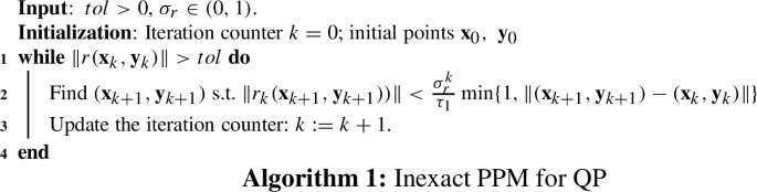
2.2 Inexact PPM
The inexact PPM has been originally analysed in [28] but we follow here the developments of [20]. We consider an approximate version of the PPM scheme in (8) where \(({\textbf{x}}_{k+1}, {\textbf{y}}_{k+1})\) satisfies the criterion \((A_1)\) in [20], i.e.,
Theorem 2.1 summarizes the results we are going to use in this work (the statements are specialized for our case):
Theorem 2.1
-
1.
The sequence \(\{({\textbf{x}}_{k},{\textbf{y}}_{k})\}_{k \in {\mathbb {N}}}\) generated by the recursion in (8) and using as inexactness criterion (a relaxed version of (10))
$$\begin{aligned} \Vert ({\textbf{x}}_{k+1}, {\textbf{y}}_{k+1})-{\mathcal {P}}({\textbf{x}}_{k}, {\textbf{y}}_{k})\Vert \le \varepsilon _k, \textrm{where } \sum _{k=0}^{+\infty } \varepsilon _k < \infty , \end{aligned}$$is bounded if and only if Assumption 1 holds. Moreover it converges to a point \(({\textbf{x}}^{*},{\textbf{y}}^{*}) \in T_{{\mathcal {L}}}^{-1}(0)\) and
$$\begin{aligned} 0 = \lim _{k \rightarrow \infty } \Vert (I-{\mathcal {P}})({\textbf{x}}_{k},{\textbf{y}}_{k})\Vert =\lim _{k \rightarrow \infty } \Vert ({\textbf{x}}_{k+1},{\textbf{y}}_{k+1})-({\textbf{x}}_{k},{\textbf{y}}_{k})\Vert , \end{aligned}$$see [28, Th. 1].
-
2.
Suppose that
$$\begin{aligned} \begin{aligned}&\exists \; a>0, \; \exists \; \delta >0: \; \forall {\textbf{w}} \in B(0,\delta ), \; \forall {\textbf{z}} \in T^{-1}_{{\mathcal {L}}}({\textbf{w}}) \\&\hbox { we have } dist({\textbf{z}}, T_{{\mathcal {L}}}^{-1}(0)) \le a \Vert {\textbf{w}}\Vert . \end{aligned} \end{aligned}$$(11)Then, the sequence \(\{({\textbf{x}}_{k},{\textbf{y}}_{k})\}_{k \in {\mathbb {N}}}\) generated by the recursion in (8) using as inexactness criterion (10), is such that \(dist(({\textbf{x}}_{k},{\textbf{y}}_{k}),T_{{\mathcal {L}}}^{-1}(0))\rightarrow 0\) linearly. Moreover, the rate of convergence is bounded by \(a/(a^2+ (1/\max \{\rho ,\delta \})^2)^{1/2}\), i.e.,
$$\begin{aligned} \lim \sup _{k \rightarrow \infty } \frac{dist(({\textbf{x}}_{k+1},{\textbf{y}}_{k+1}),T_{{\mathcal {L}}}^ {-1}(0))}{dist(({\textbf{x}}_{k},{\textbf{y}}_{k}),T_{{\mathcal {L}}}^{-1}(0))} \le \frac{a}{(a^2+(1/\max \{\rho ,\delta \})^2)^{1/2}}<1, \end{aligned}$$(12)see [20, Th. 2.1].
Remark 2.1
Since the operators \(T_{{\mathcal {L}}}\) and \(T_{{\mathcal {L}}}^{-1}\) are polyhedral variational inequalities, they satisfy condition (11), see [9, Sec. 3.4].
2.3 Practical Stopping Criteria for Inexactness
As stated in Item 2. of Theorem 2.1, in order to guarantee linear convergence, it is sufficient to impose algorithmically the condition in (10). In particular, using (7) or (9) and the fact that, in general, it holds
see [9, Sec. 2.1], we can define the following natural residuals (used also in [7, 19]):
and
The following Lemma 2.2 summarizes some important properties of the natural residuals (13) and (14).
Lemma 2.2
The natural residuals satisfy the following properties:
-
1.
\(dist(0,T_{{\mathcal {L}}}^{-1}({\textbf{x}},{\textbf{y}}))=O(\Vert r({\textbf{x}},{\textbf{y}})\Vert )\);
-
2.
There exists a constant \(\tau _1 >0\) s.t.
$$\begin{aligned} {\Vert ({\textbf{x}}, {\textbf{y}})-{\mathcal {P}}({\textbf{x}}_{k}, {\textbf{y}}_{k})\Vert } \le \tau _1 \Vert r_k({\textbf{x}},{\textbf{y}})\Vert {\hbox { for all } ({\textbf{x}},{\textbf{y}}) \in {\mathbb {R}}^{d+m}}. \end{aligned}$$
Proof
Part 1. follows using [24, Th. 18]. Part 2. follows using an analogous reasoning as that in the proof [19, Prop. 2, Item 3.] which, in turn, is based on [24, Th. 20] and the fact that D is convex. \(\square \)
In Algorithm 1 we present the particular form of the inexact PPM considered in this work.
3 Primal-Dual IPM for Proximal Point Evaluations
For problem (RP) let us introduce the Lagrangian
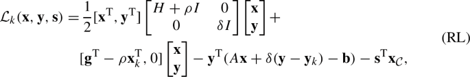
where \({\textbf{s}} \in {\mathbb {R}}^{|{\mathcal {C}}|}\) and \({\textbf{s}}\ge 0\). Using (RL), we write the KKT conditions
We can then write the dual form of problem (RP) as
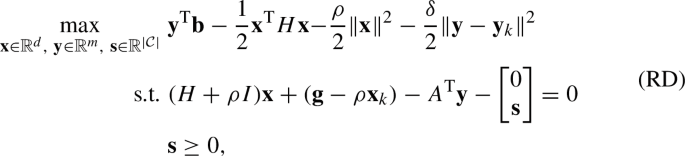
where we used the fact that \(A{\textbf{x}}+\delta {\textbf{y}}={\textbf{b}}+\delta {\textbf{y}}_k\).
In this work we consider an infeasible primal dual IPM for the solution of the problem (RP), see Algorithm 2. In particular, this is obtained considering the following Regularized Lagrangian Barrier function
We write the corresponding KKT conditions
Setting \(s_i = \frac{\mu }{x_i}\) for \(i \in {\mathcal {C}}\), we can then consider the following IPM map
where \(\sigma \in (0,1)\) is the barrier reduction parameter. A primal-dual Interior-Point Method applied to the problems (RP)-(RD), is based on applying Newton iterations to solve a nonlinear problem of the form
A Newton step for (15) from the current iterate \(({\textbf{x}},{\textbf{y}}, {\textbf{s}})\) is obtained by solving the system
Eliminating the variable \(\varDelta {\textbf{s}}\) we obtain the linear system
where \(\varTheta ^\dagger ={{{\,\textrm{diag}\,}}}((0, \dots ,0); {\textbf{x}}^{-1}_{{\mathcal {C}}}{\textbf{s}})\), \(\xi _d^1:=[(\xi _d)_1,\dots , (\xi _d)_{\bar{d}} ]^\textrm{T}\) and
\(\xi _d^2:=[(\xi _d)_{\bar{d}+1},\dots , (\xi _d)_{{d}} ]^\textrm{T}\).
In Algorithm 2 we report the IPM scheme for problem (RP). The method has a guaranteed polynomial convergence [31, Chap. 6] (cfr. also [1, 11, 12, 18]). For notational simplicity we consider the case \({\mathcal {C}}=\{1,\dots ,d\}\). To this aim, we also define

3.1 The Proximal Stabilized-Interior Point Algorithm (PS-IPM)
In Algorithm 3 we present our proposal in full detail.
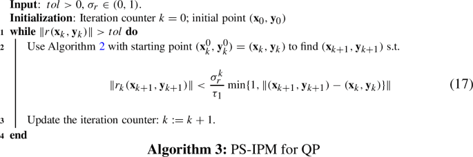
Two comments are in order at this stage.
-
1.
It is important to observe that the warm starting strategy of starting Algorithm 2 from the previous PPM approximation \(({\textbf{x}}_{k}, {\textbf{y}}_{k})\) is justified by the fact that
$$\begin{aligned} \begin{aligned}&\Vert {\mathcal {P}}({\textbf{x}}_k,{\textbf{y}}_k) -({\textbf{x}}_k,{\textbf{y}}_k) \Vert \\&\quad \le \Vert {\mathcal {P}}({\textbf{x}}_k,{\textbf{y}}_k) -{\mathcal {P}}({\textbf{x}}_{k-1},{\textbf{y}}_{k-1}) \Vert + \Vert {\mathcal {P}}({\textbf{x}}_{k-1},{\textbf{y}}_{k-1}) -({\textbf{x}}_{k},{\textbf{y}}_k) \Vert \\&\quad \le \eta \Vert ({\textbf{x}}_k,{\textbf{y}}_k) -({\textbf{x}}_{k-1},{\textbf{y}}_{k-1}) \Vert + \Vert {\mathcal {P}}({\textbf{x}}_{k-1},{\textbf{y}}_{k-1}) -({\textbf{x}}_{k},{\textbf{y}}_k) \Vert , \end{aligned} \end{aligned}$$(18)where, in the second inequality, \(\eta \) is the Lipschitz constant of the proximal operator (see [19, Theorem 4]). Since the inexact PPM converges we have that
$$\begin{aligned} \Vert {\mathcal {P}}({\textbf{x}}_{k-1},{\textbf{y}}_{k-1}) -({\textbf{x}}_{k},{\textbf{y}}_k) \Vert \rightarrow 0 \hbox { and } \Vert ({\textbf{x}}_k,{\textbf{y}}_{k}) -({\textbf{x}}_{k-1},{\textbf{x}}_{k-1}) \Vert \rightarrow 0, \end{aligned}$$and hence \( \Vert {\mathcal {P}}({\textbf{x}}_k,{\textbf{y}}_k) -({\textbf{x}}_k,{\textbf{y}}_k) \Vert \rightarrow 0\). Such observation suggests that, eventually, \( \Vert {\mathcal {P}}({\textbf{x}}_k,{\textbf{y}}_k) -({\textbf{x}}_k,{\textbf{y}}_k) \Vert \) will become sufficiently small so that the fast final convergence of IPM holds immediately and the IPM converges fast. As a result, we expect that each proximal subproblem will need a non-increasing number of IPM iterations to be solved. Indeed, we observe this behaviour in practice: typically after the first or second proximal iteration each subsequent proximal subproblem takes only two or one IPM iterations to converge (see Sect. 5.2).
-
2.
The IPM Algorithm 2 uses (17) as a stopping condition.
4 Slack Formulation and Preconditioning
The presence of proximal point regularization brings several advantages to the IPM. One of them is bounding the spectrum of the matrices in Newton system [2, 3, 14, 23]. In this section, we will show how this may be combined with the replications of the variables involved in the inequality constraints to alleviate the inherent numerical instability which originates from the IPM scaling matrix \(\varTheta \).
For the sake of simplicity, in this section, we assume that in (1) all variables have nonnegative constraints, i.e., \(\bar{d}=0\). Then, using variables replication, we get the following slack formulation [11, Sec. 6] of the original problem (1):
In this case the IPM map (15) can be written as
Using (20), the corresponding Newton system (see also Eq. (16)), can be expressed as
where \(\varTheta = ZS^{-1}\). For the convenience of the reader we also report, in the following, the explicit expressions of the IPM residuals: the natural PPM residual in (13) reads as
whereas the residual in (14) becomes
4.1 Solution of the Newton System
In this section we will study in details the solution of the linear system (21) when reordered and symmetrized as follows:
To this aim, let us partition the matrix \({\mathcal {N}}(\varTheta )\) as
where
Before continuing, let us observe that, under suitable hypothesis, the solution of a linear system of the form
can be obtained solving
Since the linear systems involving \(N_{11}(\varTheta )\) are easily solvable, using (23), the overall solution of the linear system (22) can be obtained from the following two ancillary ones:
where \(S(\varTheta )\) is the Schur complement
It is important to observe that, at this stage, the reasons to go through the current reformulation of the problem are not completely apparent: we essentially doubled the dimension of the primal variables ending up with the necessity of solving linear systems involving a Schur complement, see equation (25), which has exactly the same sparsity pattern as the standard (symmetrized) Newton system
cfr. Equation (16).
In the following Remarks 4.1 and 4.2 we highlight the advantages given by the current reformulation of the Newton system showing, in essence, that the formulation in (25) allows better preconditioner re-usage than in the standard formulation (26). To this aim, as it is customary in IPM methods, let us suppose that
where \(\mu \) is the average complementarity product at any given IPM iteration. Using the above assumption, we obtain
From Eq. (27) the main advantage of dealing with the formulation (25) of the Schur complement becomes more apparent: whilst the elements of the diagonal IPM matrix appearing in \({\mathcal {N}}_C(\varTheta )\) are such that \(\varTheta ^{-1}_{ii} \in (0,+\infty )\) when \(\mu \rightarrow 0\), the diagonal elements appearing in the Schur complement (25) belong to the interval \((\frac{\rho }{\delta \rho +1}, \frac{1}{\delta })\) when \(\mu \rightarrow 0\).
Remark 4.1
When \(\mu \rightarrow 0\), for the variables which have been identified as active or inactive by the PS-IPM, see Algorithm 3, we have that
and such values are expected to remain unchanged in the following PS-IPM steps. This suggests that, when close enough to convergence, any computed approximation of the matrix \(S(\varTheta )\) may be used as an effective preconditioner also for subsequent PS-IPM steps.
In Lemma 4.1 we show that the regularization parameters \((\rho ,\delta )\) act as attenuation coefficients, see (29), for the variations \({\widehat{\varTheta }}^{-1}_{ii} -\varTheta ^{-1}_{ii}\) where \({\widehat{\varTheta }}^{-1}\) and \(\varTheta ^{-1}\) are two IPM matrices obtained, respectively, in two different IPM iterations.
Lemma 4.1
Define
and
Then,
Proof
From direct computation we have
Then,
and the thesis follows using the definitions of \(S(\varTheta )\) and \({\mathcal {N}}_C(\varTheta )\). \(\square \)
Remark 4.2
Suppose we computed a preconditioner for \({S}(\varTheta )\), e.g., an incomplete factorization. Equation (28) shows that any accurate preconditioner for \(S(\varTheta )\) approximates \({S}({\widehat{\varTheta }})\) better than an analogous preconditioner for \({{\mathcal {N}}}_{C}(\varTheta )\) would approximate \({{\mathcal {N}}}_{C}({\widehat{\varTheta }})\).
Moreover, from (29), we can observe that the variations \((D_{A})_{ii}\), and hence the variation \(\Vert {S}({\widehat{\varTheta }})-S(\varTheta )\Vert _2\) of the overall Schur complement, are negatively correlated with the regularization parameters \((\rho , \delta )\). Then, it has to be expected that the computed preconditioner for \(S(\varTheta )\) would be yet an effective preconditioner for the matrix \({S}({\widehat{\varTheta }})\) if the regularization parameters \((\rho , \delta )\) are sufficiently large.
On the other hand, according to (12), the rate of convergence of PPM correlates inversely with the regularization parameters \((\rho , \delta )\).
As a result of the above discussion, we are able to unveil a precise interaction between the computational footprint related to the necessity of re-computing preconditioners and the rate of convergence of the PS-IPM with the obvious benefit to allow a predictable tuning of such trade-off (see Sect. 5.3).
Finally, since \(\lim _{(\rho ,\delta )\rightarrow (0,0)}(\delta I + (\varTheta ^{-1}+\rho I )^{-1})^{-1}=\varTheta ^{-1}\), we have that
indicating the fact that the re-usability of preconditioners for \({\mathcal {N}}_{C}(\varTheta )\) can be assessed as a limit case of the re-usability of preconditioners for \(S(\varTheta )\).
To conclude this section, in Theorem 4.1, we analyse in more detail the eigenvalues of the matrix \({S}({\varTheta })^{-1}{S}({\widehat{\varTheta }})\). Indeed, supposing we have computed an accurate preconditioner for \({S}({\varTheta })\), then, the eigenvalues of \({S}({\varTheta })^{-1}{S}({\widehat{\varTheta }})\) may be considered as a measure of the effectiveness of such preconditioner when used as preconditioner for \({S}({\widehat{\varTheta }})\): the results there contained will further confirm that a high quality preconditioner is expected when the matrix \(D_A\) has small diagonal elements, see (30). In this case, indeed \({S}({\varTheta })^{-1}{S}({\widehat{\varTheta }})\) has a highly clustered spectrum.
Theorem 4.1
Let us define
Then, the matrix \({S}({\varTheta })^{-1}{S}({\widehat{\varTheta }})\) has the eigenvalue \(\eta =1\) with multiplicity at least m whereas, the other eigenvalues, are s.t.
Proof
To analyse the eigenvalues we consider the problem
i.e.,
If \(\eta =1\), we obtain that any vector of the form \([0,{\textbf{u}}_2]\) is a solution of (31) and hence the multiplicity of eigenvalue 1 is at least m. Let us suppose \(\eta \ne 1\). Always from (31) we obtain \(A{\textbf{u}}_1=\delta {\textbf{u}}_2\) and hence, using the equality
we obtain
Thesis follows from (32) using the definition of \(D_A\), \(H_{A,\varTheta , \delta , \rho }\) and the fact that both are symmetric matrices. \(\square \)
4.1.1 Further Schur Complement Reduction
In some particular cases, using once more (23), it might be computationally advantageous to further reduce the solution of the linear system in (24) to a smaller linear system involving its Schur complement. Among other situations, this is the case of IPM matrices coming from problems of the form (19) for which H is diagonal, e.g., \(H=0\) (LP case). In this section we prove a similar result to Lemma 4.1 when the involved matrices are the Schur complements of the linear systems (25) and (26). To this aim and for the sake of simplicity, we consider the case \(H=0\) and define \(L_1(\varTheta )\) as the Schur complement of (25), i.e.,
whereas we define \(L_2(\varTheta )\) as the Schur complement of (26), i.e.,
Moreover, considering diagonal scaling matrices \({\widehat{\varTheta }}^{-1}\) and \(\varTheta ^{-1}\) obtained, respectively in two different IPM iterations, we have
whereas
We are ready to state Lemma 4.2, which guarantees that also when operating a further reduction to the Schur complement in (25), the regularization parameters \((\rho ,\delta )\) act as dumping factors for the changes in the diagonal matrix \(|\varDelta _{2,{\widehat{\varTheta }},\varTheta }|\).
Lemma 4.2
With the notation introduced above, we have
and
Proof
From direct computation, we have that
from which, observing that \((\varDelta _{2,{\widehat{\varTheta }},\varTheta })_{ii}=\frac{{\widehat{\varTheta }}_{ii}^{-1} - {\varTheta }_{ii}^{-1}}{({\widehat{\varTheta }}^{-1}_{ii}+\rho )({\varTheta }^{-1}_{ii}+\rho )}\), (34) follows. The second part of the statement follows observing that
where in the last inequality we used (34). \(\square \)
5 Numerical Results
Aim of this section is to present the computational results obtained using Algorithm 3 (PS-IPM) when solving a set of small to large scale linear and convex quadratic problems. All the numerical results presented in this section are performed using a Dell PowerEdge R740 running Scientific Linux 7 with \(4 \times \) Intel Gold 6234 3.3 G, 8C/16T, 10.4GT/s, 24.75 M Cache, Turbo, HT (130W) DDR4-2933. Our implementation closely follows the one from [25] and is written in Matlab® R2022a (available at the website https://github.com/StefanoCipolla/PS-IPM). Concerning the choice of the initial guess, we use the same initial point as in [25, Sec. 5.1.3], which, in turn, is based on the developments in [22]. Concerning instead the choice of the parameters in Algorithm 3, we set \(\sigma _r = 0.7\). Moreover, to prevent wasting time on finding excessively accurate solutions in the early PPM sub-problems, we replace (17) with
Indeed, in our computational experience, we have found that driving the IPM solver to a high accuracy in the initial PPM iterations is unnecessary and, usually, leads to a significant deterioration of the overall performance. Finally, we set as regularization parameters \(\delta = \rho \), where
see [25]. The remainder of this section is organized as follows.
In Sect. 5.1 we present the comparison of PS-IPM with Matlab®’s linprog (‘Algorithm’: ‘interior-point’) and quadprog (‘Algorithm’: ‘interior-point-convex’). For the fairness of comparison and to be sure that all the compared algorithms are working on the same dataset, we use the option ‘Preprocess’: ‘none’ in linprog (the same option is not available for quadprog, which always performs a Preprocess phase). Moreover, both solvers use a multiple centrality corrections strategy to find the search direction, see [15]. For this reason and for the fairness of comparison, we use the same strategy in our PS-IPM implementation. This issue represents the main point where practical implementation deviates from the theory in order to gain computational efficiency. Concerning the stopping criteria, always for the fairness of the comparison, instead of using the natural residual (13), we stop the iterations of Algorithm 3 using the same stopping criteria of linprog & quadprog, i.e.,
where
and
In Sect. 5.2 we present the comparison of PS-IPM with IP-PMM [25]. In our PS-IPM implementation, analogously to [25], in order to find the search direction, we employ a widely used predictor–corrector method [22]. Also in this case, this issue represents the main point where practical implementation deviates from the theory in order to gain computational efficiency and is here used for the fairness of comparison with IP-PMM. Concerning the stopping criterion, always for the fairness of the comparison with IP-PMM, instead of using the natural residual (13), we stop the iterations of Algorithm 3 when
and when \(\hbox {tol} =10^{-6}\).
As highlighted in the above discussion, the choice of presenting separate comparison is due essentially to the fact that linprog &quadprog use different stopping criteria and different strategies for generating the search directions w.r.t. IP-PMM and, for the sake of presenting trustworthy comparative results, we replicated such features in our PS-IPM implementation.
In both, Sects. 5.1 and 5.2, we solve the (symmetrized) Newton linear systems (16), using Matlab®’s ldl factorization. The factorization threshold parameter is set equal to the regularization parameter [see (35)] and is incremented by a factor 10 if numerical instabilities are detected in the obtained solution of the given linear system. Finally, it is important to note that the reported computational times in this work are just indicative of the relative performance rather than the absolute ones. Indeed, each call of the Matlab®’s ldl (wich uses MA57 [10]) requires an Analysis Phase [10, Sec. 6.2] which, in an optimal implementation, can be performed just once in the pre-processing phase since the sparsity pattern of the Newton matrices does not change during the IPM iterations. Moreover, from the practical point of view, it is important to note that, if on the one hand choosing the threshold parameter equal to the regularization accelerates the ldl routine for the Newton systems arising in Algorithm 2, on the other, the presence of such regularization terms stabilizes it. For this reason, we expect for Algorithm 3 similar stability and robustness properties when compared to IP-PMM, which, in turn, shows improved robustness capabilities with respect to the non regularized version (see [11, 25]).
Finally, in Sect. 5.3, we present the numerical results relative to Sect. 4. In particular, we present here a series of numerical results aiming to showcase to which extent the theory developed in Sect. 4 would allow the reusability of a given factorization as preconditioner for Krylov iterative solvers [30]. To this aim, in Sect. 5.3.1, we consider the case when the linear system involving \(S(\varTheta )\) in (24) is solved without further reduction to Schur complement, whereas, in Sect. 5.3.2, we present the numerical results when such further reduction is considered, see Sect. 4.1.1 for the theoretical details. For the sake of readability, we postpone the detailed description of the computational frameworks used to the particular sections. Moreover, we point out that in Sect. 5.3 we use the same stopping criterion, see (36), and the same predictor-corrector strategy as the one used in Sect. 5.2.
Dataset For the small/medium scale linear programming problems, the test set consists of 98 linear programming problems from the Netlib collection. For the small/medium scale convex quadratic problems, the test set consists of 122 problems from the Maros-Mészáros collection [21]. For the large scale linear programming problems, the test set consists of 19 problems coming from Netlib, Qaplib and Mittelmann’s collection.
For the sake of completeness, in Table 1, we report the dimensions and the number of non-zeros of the largest instances considered in this work [when the problems are formulated as in (1)].
Before showing the detailed comparison results, we start by briefly showcasing the theory developed in Sects. 2 and 3. In particular, in Fig. 1a, b, we report the details of the run of Algorithm 3 on the problems 25FV47 and PILOT87 from the Netlib collection. As the figures show, accordingly to (12) in Theorem 2.1, the rate of convergence of PPM decreases when the regularization parameter is increased (lower panels of Fig. 1a, b). Moreover, accordingly to (18), the number of IPM iterations needed to solve the PPM sub-problems is non-increasing when the PPM iterations proceed (somehow our choice of the parameters amplifies this feature since in the majority of PPM iterations just one IPM sweep is enough to meet the inexactness criterion, see upper panels in Fig. 1a, b).

Theory showcase. Upper Panels: PPM Iterations and IPM Iterations. Lower Panels: Behaviour of residuals
5.1 PS-IPM Versus Matlab®’s Solvers
In this section we compare the performance of Algorithm 3 (PS-IPM) with that of Matlab®’s IPM-based solvers. To this aim, we present in Fig. 2a–c the performance profiles of our proposal, PS-IPM, when compared to Matlab®’s linprog and quadprog. Moreover, in Table 2 we report the overall statistics of the performance of two methods.

PS-IPM versus Matlab®’s solvers: overall statistics
As already mentioned at the beginning of this section, we compare the two methods without using the pre-solved version of the problem collection (i.e. allowing rank-deficient matrices). Our proposal reaches the required accuracy on all the problems whereas Matlab®’s solvers do not solve a total of six problems. Hence, as expected, one of the benefits of the PPM framework becomes immediately obvious: the introduction of the regularization alleviates the rank deficiency of the constraint matrix while guaranteeing convergence. Moreover, in the small/medium setting, despite PS-IPM might not be the best performer on particular instances, it always outperforms linprog and quadprog in terms of overall execution time, see Fig. 2a, b and Table 2. Instead, as Fig. 2c clearly shows, PS-IPM is undoubtedly the best performer in terms of robustness and efficiency on the large scale dataset. All the obtained objective values from the methods are comparable.
5.2 PS-IPM Versus IP-PMM [25]
In this section we compare the performance of Algorithm 3 (PS-IPM) with that of IP-PMM [25]. To this aim, we report in Fig. 3a–c the performance profiles of PS-IPM when compared IP-PMM. Moreover, in Table 3, we report the overall statistics of the performance of two methods on the considered datasets. Our proposal reaches the required accuracy on all the problems whereas IP-PMM does not solve a total of two problems. Hence, as expected, our proposal has the same robustness capabilities as IP-PMM. On the other hand, as revealed from the Fig. 3a–c, the framework here proposed outperforms consistently IP-PMM in terms of IPM iterations (right panels). This fact is indeed always reflected in a reduction of the execution time (left panels and see also Table 3). All the obtained objective values from the two methods are comparable also in this case.

PS-IPM versus PMM: performance profiles
Finally, in order to give a measure of the number of IPM sweeps performed per PPM iteration when solving large scale problems, we report in Fig. 4 the ratio “Interior Point Iterations/Proximal Point Iterations” (\(\frac{\hbox {IPM} \; \hbox {It}.}{\hbox {PPM} \; \hbox {It}.}\)). Clearly, lower ratios are indicative of the fact that, in average, fewer IPM iterations have been performed per PPM step. The figure further confirms the fact that thanks to the warm starting in Algorithm 3 and the property (18), the average number of IPM sweeps per PPM iteration remains bounded by the worst case factor of four also for larger problems than those corresponding to Fig. 1a, b (see Table 4 for details of the performance of PS-IPM on the large scale LPs considered).
5.3 PS-IPM and Krylov Solvers
In this section we present the computational results obtained using Algorithm 3 when the problem is reformulated as in (19) and the corresponding linear systems arising from the PS-IPM subproblems are solved using (24) in conjunction with Krylov iterative solvers [30]. More in details, all the computational results presented here are devoted to showcase the theory developed in Sect. 4.1 and, in particular, to show that PS-IPM requires, in practice, a number of factorizations (short-handed as Fact. in the following) equal to a fraction of the IPM iterations, delivering hence considerable savings of computational time for problems where the factorization footprint is dominant. It is important to note that, in this context, a given factorization is not used any more as back-solver for a given Newton system but, rather, as preconditioner for suitable Krylov methods. In the following discussions and through all this section, we will use the ratio “Interior Point Iterations/ Factorizations” (\(\frac{\hbox {IPM It}.}{\hbox {Fact}.}\)), as a measure of the frequency at which the preconditioner is recomputed: higher ratios are indicative of the fact that the same factorization has been used successfully by a larger number of IPM iterations. Moreover, we will use the ratio “Krylov Iterations/Factorizations” (\(\frac{\hbox {Krylov} \; \hbox {It}.}{\hbox {Fact}.}\)) as a measure of how much the Krylov iterative solver is able to successfully exploit a given preconditioner: higher ratios are indicative of the fact that the same factorization has been used successfully to solve a larger number of linear systems.

Average IPM sweeps per PPM iteration
5.3.1 Strategy 1: Solution of the Linear System (24) Without Reduction to Schur Complement
Computational framework’s details In this section, for the solution of the linear system (24), we use GMRES [29] without restart and \(\hbox {MaxIt}=100\). Moreover, as suggested in the discussion in Sect. 4.1, as preconditioner of a given Schur complement \(S({\widehat{\varTheta }})\), we use the ldl decomposition of \(S({\varTheta })\) computed in a previous PS-IPM iteration with factorization threshold parameter set equal to the regularization parameter, see (35). It is important to note that when GMRES is applied to a non-normal matrix its convergence behaviour is not fully determined by the spectral distribution of the matrix, or better, this spectral distribution is completely irrelevant [16]. Nevertheless, when \(\Vert S(\varTheta ) - S({\widehat{\varTheta }})\Vert _2 \) is small, we expect the matrix \({S}({\varTheta })^{-1}{S}({\widehat{\varTheta }})\) to be close to the identity. In this case, and in general for symmetric matrices, the spectral distribution is fully descriptive of GMRES behaviour [30, Cor. 6.33] and hence we expect GMRES to behave accordingly to the spectrum of the preconditioned matrix as in Theorem 4.1. As previously mentioned, we factorize the Schur complement in (25) using Matlab®’s ldl routine and, in our experiments, this factorization is recomputed if in the current PS-IPM step, GMRES has performed more than the \(51\%\) of the maximum allowed iterations in the solution of at least one of the two predictor-corrector systems. The stopping (absolute) tolerance for GMRES is set as \(\min \{10^{-1},0.8\mu \}\) where \(\mu \) is the current duality gap (the interested reader can see [8] for a recent analysis of inexact predictor-corrector schemes).
Obtained numerical results In Tables 5 and 6 we report the details for the largest instances of the medium-size LPs and QPs already considered in Sects. 5.1 and 5.2, see Table 1, when varying the stopping tolerance (tol) and when the regularization parameters have been suitably increased w.r.t. the ones used in the aforementioned sections in order to better showcase the developed theory.
The results obtained confirm that the ratio \(\frac{\hbox {IPM} \; \hbox {It}.}{\hbox {Fact}.}\) remains roughly in the interval (2.5, 6) for all the considered problems, see also Fig. 5, confirming, in general, that our proposal allows a small number of preconditioner re-computations. Moreover, as it becomes apparent from Fig. 5, when switching from \(\hbox {tol}=10^{-5}\) to \(\hbox {tol}=10^{-7}\) or \(\hbox {tol}=10^{-8}\) the above mentioned ratio tends to increase for the problems PILOT87,CVXQP1,LISWET1, LISWET10,POWELL20,SHIP12L (the same happens for the ratio \(\frac{\hbox {Krylov} \; \hbox {It}.}{\hbox {Fact}.}\)) essentially indicating that the computed preconditioners have been used to solve successfully a larger number of linear systems during the optimization procedure.
Indeed, this is in accordance with the observation carried out in Remark 4.1 of Sect. 4.1 regarding the fact that, when close enough to convergence, less re-factorizations are needed due to the convergence behaviour of the IPM contribution \(\varTheta ^{-1}\) to the matrix \(S(\varTheta )\) [see Eq. (25)].

Average IPM and Krylov It. per factorization
In Tables 7 and 8 we report the details for the instances of large size considered in Sect. 5.2 when the regularization is increased, respectively, by a factor \(f=10\) and \(f=500\) if compared to the regularization parameters used in Table 4.
In this case, the ratio \(\frac{\hbox {IPM} \; \hbox {It}.}{\hbox {Fact}.}\) remains bounded from below by a factor strictly greater than two, clearly indicating that, also in this case, the number of necessary factorizations to optimize successfully a given problem is just a fraction of the total IPM iterations. This fact could lead to reduced computational times for instances in which the effort related to the factorization is dominant, when compared to approaches where the ldl factorization is recomputed at each IPM iteration in order to solve the Newton system (see, e.g., the first part of this work).
As it becomes apparent from Fig. 6, when increasing the regularization parameters, the ratios \(\frac{\hbox {IPM} \; \hbox {It}.}{\hbox {Fact}.}\) and \(\frac{\hbox {Krylov} \; \hbox {It}.}{\hbox {Fact}.}\) tend to increase for the majority of the problems, indicating that the number of computed factorizations can be further reduced. Indeed, this is in accordance with the observation carried out in Remark 4.2 of Sect. 4.1 regarding the fact that the diagonal variations \((D_{A})_{ii}\) of the Schur complements \(S(\varTheta )\) are inversely proportional to the regularization parameters \((\rho , \delta )\) [see Eq. (29)].
Moreover, to further assess the robustness of our proposal on large scale problems, we complement the dataset used until now with additional large scale LP instances. We report in Table 9 the corresponding details.
5.3.2 Strategy 2: Solution of the Linear System (24) with Reduction to Schur Complement
Computational framework’s details When a further reduction to Schur complement is considered for the solution of the linear system (33), see Sect. 4.1.1, we propose to use the Preconditioned Conjugate Gradient (PCG) with \(MaxIt=200\). Moreover, as suggested in the discussion carried out in Sect. 4.1.1, as preconditioner of a given \(L_1({\widehat{\varTheta }})\), we use the Cholesky decomposition of \(L_1({\varTheta })\) computed in a previous PS-IPM iteration. Analogously of what has been done in Sect. 5.3.1, we factorize a given \(L_1({\varTheta })\) as (33) using Matlab®’s chol routine and, in our experiments, this factorization is recomputed if in the current PS-IPM step, PCG has performed more than \(51\%\) of the maximum allowed iterations in the solution of at least one of the two predictor-corrector systems. The stopping (absolute) tolerance for PCG is set as \(10^{-1} \cdot \hbox {tol}\) (this choice does not guarantee in general the best performance, see [32] for a recent analysis, but it is a robust one).

Average IPM and Krylov It. per factorization
Obtained computational results Aim of this section is to show that also in the current approach the number of necessary factorizations is equal to a fraction of the total number of IPM iterations and that a further reduction to Schur complement might improve computational times when precise criteria are met. For this reason and for the sake of brevity, we present the obtained numerical results only on a selected subset of problems for which such reduced computational times are observed when compared to those presented in Sect. 5.3.1.
In Table 10 we summarize the statistics of the runs of our proposal when Newton linear systems are solved with PCG+chol.
As the results presented in Table 10 confirm, in LP problems for which the pattern of the matrix \(A^\textrm{T}A+\delta I\) is particularly sparse and/or such matrix is of small dimension, the approach considered in this section leads to improved computational times while performing a limited number of Cholesky factorizations. Indeed, as confirmed in Fig. 7, the Cholesky factors of \(A^\textrm{T}A+\delta I\) for which improved computational times are observed when compared to those presented in Sect. 5.3.1, have a consistently smaller number of non-zeros entries when compared to the LDL factors of the saddle matrix \(\begin{bmatrix} \rho I &{} A^\textrm{T} \\ A &{} -\delta I \end{bmatrix}\).

Sparsity patterns of the Cholesky factors for normal equations (top) versus sparsity of LDL factors for saddle matrices (bottom)
6 Conclusions
In this work we have clarified certain nuances of the convergence theory of primal-dual regularized Interior Point Methods (IPMs) using the inexact Proximal Point Method (PPM) framework: if on one hand this closes an existing literature gap, on the other, it sheds further light on their optimal implementation especially in the (nearly) rank deficient case of the linear constraints and/or in the large scale setting. Indeed, our convergence analysis does not require any linear independence assumption on the linear constraints nor the positive definiteness of the quadratic term. Moreover, when a direct solver can be used for the solution of the Newton system, we showed experimentally in Sect. 5.1, that the framework here proposed is competitive with Matlab®’s IPM-based solvers and, in Sect. 5.2 , that a fixed but small regularization parameter is preferred to strategies in which the regularization is driven to zero. The second part of this work has been devoted to the study of the interactions between the regularization parameters and the computational complexity of the linear algebra solvers used in IPM. In Sect. 4.1 we proposed a new preconditioning technique able to exploit regularization as a tool to reduce the number of preconditioner re-computations when an iterative solver is needed for the solution of the IPMs Newton systems. Indeed, we were able to devise general purpose preconditioners which require an update frequency inversely proportional to the magnitude of the regularization parameters. Finally, building the momentum from the correct interpretation of the primal-dual regularization parameters in connection with the overall rate of convergence of the PPM and the proposed preconditioning strategy, we were able to show the robustness and efficiency of our proposal on a class of medium and large scale LPs and QPs.
References
Al-Jeiroudi, G., Gondzio, J.: Convergence analysis of the inexact infeasible interior point method for linear optimization. J. Optim. Theory Appl. 141(2), 231–247 (2009). https://doi.org/10.1007/s10957-008-9500-5
Altman, A., Gondzio, J.: Regularized symmetric indefinite systems in interior-point methods for linear and quadratic optimization. In: Optim. Methods Softw. 11/12.1-4 (1999), pp. 275–302. https://doi.org/10.1080/10556789908805754
Armand, P., Benoist, J.: Uniform boundedness of the inverse of a Jacobian matrix arising in regularized interior-point methods. In: Math. Program. 137.1-2, Ser. A (2013), pp. 587–592. https://doi.org/10.1007/s10107-011-0498-3
Clason, C., Valkonen, T.: Introduction to nonsmooth analysis and optimization. In: arXiv (2020). https://doi.org/10.48550/ARXIV.2001.00216
Colombo, M., Gondzio, J.: Further development of multiple centrality correctors for interior point methods. Comput. Optim. Appl. 41.3, 277–305 (2008). https://doi.org/10.1007/s10589-007-9106-0
D’Apuzzo, M., De Simone, V., di Serafino, D.: On mutual impact of numerical linear algebra and large-scale optimization with focus on interior point methods. Comput. Optim. Appl. 45.2, 283–310 (2010). https://doi.org/10.1007/s10589-008-9226-1
De Marchi, A.: On a primal-dual Newton proximal method for convex quadratic programs. Comput. Optim. Appl. 81, 369–395 (2022). https://doi.org/10.1007/s10589-021-00342-y
Dexter, G., Chowdhury, A., Avron, H., Drineas, P.: On the convergence of inexact predictor-corrector methods for linear programming. In: arXiv (2022). https://doi.org/10.48550/ARXIV.2202.01756
Dontchev, A.L., Rockafellar, R.T.: Implicit Functions and Solution Mappings. Springer Monographs in Mathematics, p. xii+375. Springer, Dordrecht (2009). https://doi.org/10.1007/978-0-387-87821-8
Duff, I.S.: MA57-a code for the solution of sparse symmetric definite and indefinite systems. ACM Trans. Math. Softw. 30.2, 118–144 (2004). https://doi.org/10.1145/992200.992202
Friedlander, M.P., Orban, D.: A primal-dual regularized interior point method for convex quadratic programs. Math. Program. Comput. 4.1, 71–107 (2012). https://doi.org/10.1007/s12532-012-0035-2
Gondzio, J.: Convergence analysis of an inexact feasible interior-point method for convex quadratic programming. SIAM J. Optim. 23.3, 1510–1527 (2013). https://doi.org/10.1137/120886017
Gondzio, J.: Interior point methods 25 years later. Eur. J. Oper. Res. 218.3, 587–601 (2012). https://doi.org/10.1016/j.ejor.2011.09.017
Gondzio, J.: Matrix-free interior point methods. Comput. Optim. Appl. 51.2, 457–480 (2012). https://doi.org/10.1007/s10589-010-9361-3
Gondzio, J.: Multiple centrality corrections in a primal-dual method for linear programming. Comput. Optim. Appl. 6.2, 137–156 (1996). https://doi.org/10.1007/BF00249643
Greenbaum, A., Pták, V., Strakoš, Z.: Any nonincreasing convergence curve is possible for GMRES. SIAM J. Matrix Anal. Appl. 17.3, 465–469 (1996). https://doi.org/10.1137/S0895479894275030
Hestenes, M.R.: Multiplier and gradient methods. J. Optim. Theory Appl. 4, 303–320 (1969). https://doi.org/10.1007/BF00927673
Kojima, M., Megiddo, N., Mizuno, S.: A primal-dual infeasible interior point algorithm for linear programming. In: Math. Programming 61.3, Ser. A (1993), pp. 263–280. https://doi.org/10.1007/BF01582151
Liao-McPherson, D., Kolmanovsky, I.: FBstab: a proximally stabilized semismooth algorithm for convex quadratic programming. In: Automatica J. IFAC 113 (2020). https://doi.org/10.1016/j.automatica.2019.108801
Luque, F.J.: Asymptotic convergence analysis of the proximal point algorithm. SIAM J. Control Optim. 22.2, 277–293 (1984). https://doi.org/10.1137/0322019
Maros, I., Mészáros, C.: A repository of convex quadratic programming problems. In: Optim. Methods Softw. 11/12.1-4 (1999), pp. 671–681. https://doi.org/10.1080/10556789908805768
Mehrotra, S.: On the implementation of a primal-dual interior-point methods. SIAM J. Optim. 2.4, 575–601 (1992). https://doi.org/10.1137/0802028
Morini, B., Simoncini, V., Tani, M.: A comparison of reduced and unreduced KKT systems arising from interior point methods. Comput. Optim. Appl. 68.1, 1–27 (2017). https://doi.org/10.1007/s10589-017-9907-8
Pang, J.-S.: Error bounds in mathematical programming. In: Math. Program. 79.1-3, Ser. B (1997), pp. 299–332. https://doi.org/10.1016/S0025-5610(97)00042-7
Pougkakiotis, S., Gondzio, J.: An interior point-proximal method of multipliers for convex quadratic programming. Comput. Optim. Appl. 78.2, 307–351 (2021). https://doi.org/10.1007/s10589-020-00240-9
Rockafellar, R.T.: Augmented Lagrangians and applications of the proximal point algorithm in convex programming. Math. Oper. Res. 1.2, 97–116 (1976). https://doi.org/10.1287/moor.1.2.97
Rockafellar, R.T.: Monotone operators associated with saddle-functions and minimax problems. In: Nonlinear Functional Analysis (Proc. Sympos. Pure Math., Vol. XVIII, Part 1, Chicago, Ill., 1968). Amer. Math. Soc., Providence, R.I., (1970), pp. 241–250
Rockafellar, R.T.: Monotone operators and the proximal point algorithm. SIAM J. Control Optim. 14.5, 877–898 (1976). https://doi.org/10.1137/0314056
Saad, Y., Schultz, M.H.: GMRES: a generalized minimal residual algorithm for solving nonsymmetric linear systems. SIAM J. Sci. Stat. Comput. 7.3, 856–869 (1986). https://doi.org/10.1137/0907058
Saad, Y.: Iterative Methods for Sparse Linear Systems, 2nd edn., p. xviii528. Society for Industrial and Applied Mathematics, Philadelphia (2003). https://doi.org/10.1137/1.9780898718003
Wright, S.J.: Primal-Dual Interior-Point Methods, p. xx+289. Society for Industrial and Applied Mathematics, Philadelphia, PA (1997). https://doi.org/10.1137/1.9781611971453
Zanetti, F., Gondzio, J.: A new stopping criterion for Krylov solvers applied in interior point methods. In: SIAM J. on Sci. Comp. (Accepted)
Author information
Authors and Affiliations
Corresponding authors
Additional information
Communicated by Nobuo Yamashita.
Publisher's Note
Springer Nature remains neutral with regard to jurisdictional claims in published maps and institutional affiliations.
Rights and permissions
Open Access This article is licensed under a Creative Commons Attribution 4.0 International License, which permits use, sharing, adaptation, distribution and reproduction in any medium or format, as long as you give appropriate credit to the original author(s) and the source, provide a link to the Creative Commons licence, and indicate if changes were made. The images or other third party material in this article are included in the article’s Creative Commons licence, unless indicated otherwise in a credit line to the material. If material is not included in the article’s Creative Commons licence and your intended use is not permitted by statutory regulation or exceeds the permitted use, you will need to obtain permission directly from the copyright holder. To view a copy of this licence, visit http://creativecommons.org/licenses/by/4.0/.
About this article

Cite this article
Cipolla, S., Gondzio, J. Proximal Stabilized Interior Point Methods and Low-Frequency-Update Preconditioning Techniques. J Optim Theory Appl 197, 1061–1103 (2023). https://doi.org/10.1007/s10957-023-02194-4
Received:
Accepted:
Published:
Issue Date:
DOI: https://doi.org/10.1007/s10957-023-02194-4
Keywords
- Interior point methods
- Proximal point methods
- Regularized primal-dual methods
- Convex quadratic programming