Abstract
We propose an approach for improving sequence modeling based on autoregressive normalizing flows. Each autoregressive transform, acting across time, serves as a moving frame of reference, removing temporal correlations and simplifying the modeling of higher-level dynamics. This technique provides a simple, general-purpose method for improving sequence modeling, with connections to existing and classical techniques. We demonstrate the proposed approach both with standalone flow-based models and as a component within sequential latent variable models. Results are presented on three benchmark video datasets and three other time series datasets, where autoregressive flow-based dynamics improve log-likelihood performance over baseline models. Finally, we illustrate the decorrelation and improved generalization properties of using flow-based dynamics.
Find the latest articles, discoveries, and news in related topics.Avoid common mistakes on your manuscript.
1 Introduction
Data often contain sequential structure, providing a rich signal for learning models of the world. Such models are useful for representing sequences (Li and Mandt 2018; Ha and Schmidhuber 2018) and planning actions (Hafner et al. 2019; Chua et al. 2018). Recent advances in deep learning have facilitated learning sequential probabilistic models directly from high-dimensional data (Graves 2013), like audio and video. A variety of techniques have emerged for learning deep sequential models, including memory units (Hochreiter and Schmidhuber 1997) and stochastic latent variables (Chung et al. 2015; Bayer and Osendorfer 2014). These techniques have enabled sequential models to capture increasingly complex dynamics. In this paper, we explore the complementary direction, asking can we simplify the dynamics of the data to meet the capacity of the model? To do so, we aim to learn a frame of reference to assist in modeling the data.
Frames of reference are an important consideration in sequence modeling, as they can simplify dynamics by removing redundancy. For instance, in a physical system, the frame of reference that moves with the system’s center of mass removes the redundancy in displacement. Frames of reference are also more widely applicable to arbitrary sequences. Indeed, video compression schemes use predictions as a frame of reference to remove temporal redundancy (Oliver 1952; Agustsson et al. 2020; Yang et al. 2021). By learning and applying a similar type of temporal normalization for sequence modeling, the model can focus on aspects that are not predicted by the low-level frame of reference, thereby simplifying dynamics modeling.
We formalize this notion of temporal normalization through the framework of autoregressive normalizing flows (Kingma et al. 2016; Papamakarios et al. 2017). In the context of sequences, these flows form predictions across time, attempting to remove temporal dependencies (Srinivasan et al. 1982). Thus, autoregressive flows can act as a pre-processing technique to simplify dynamics. We preview this approach in Fig. 1, where an autoregressive flow modeling the data (top) creates a transformed space for modeling dynamics (bottom). The transformed space is largely invariant to absolute pixel value, focusing instead on capturing deviations and motion.
We empirically demonstrate this modeling technique, both with standalone autoregressive normalizing flows, as well as within sequential latent variable models. While normalizing flows have been applied in sequential contexts previously, our main contributions are in (1) showing how these models can act as a general pre-processing technique to improve dynamics modeling, (2) empirically demonstrating log-likelihood performance improvements, as well as generalization improvements, on three benchmark video datasets and time series data from the UCI machine learning repository. This technique also connects to previous work in dynamics modeling, probabilistic models, and sequence compression, enabling directions for further investigation.

Sequence modeling with autoregressive flows. Top: Pixel values (solid) for a particular pixel location in a video sequence. An autoregressive flow models the pixel sequence using an affine shift (dashed) and scale (shaded), acting as a frame of reference. Middle: Frames of the data sequence (top) and the resulting “noise” (bottom) from applying the shift and scale. The redundant, static background has been largely removed. Bottom: The noise values (solid) are modeled using a base distribution (dashed and shaded) provided by a higher-level model. By removing temporal redundancy from the data sequence, the autoregressive flow simplifies dynamics modeling
2 Background
2.1 Autoregressive models
Consider modeling discrete sequences of observations, \({\mathbf {x}}_{1:T} \sim p_{{\text {data}}} ({\mathbf {x}}_{1:T})\), using a probabilistic model, \(p_\theta ({\mathbf {x}}_{1:T})\), with parameters \(\theta \). Autoregressive models (Frey et al. 1996; Bengio and Bengio 2000) use the chain rule of probability to express the joint distribution over time steps as the product of T conditional distributions. These models are often formulated in forward temporal order:
Each conditional distribution, \(p_\theta ({\mathbf {x}}_t | {\mathbf {x}}_{<t})\), models the dependence between time steps. For continuous variables, it is often assumed that each distribution takes a simple form, such as a diagonal Gaussian: \(p_\theta ({\mathbf {x}}_t | {\mathbf {x}}_{<t}) = {\mathcal {N}} ({\mathbf {x}}_t ; \varvec{\mu }_\theta ({\mathbf {x}}_{<t}), {{\,\mathrm{diag}\,}}(\varvec{\sigma }^2_\theta ({\mathbf {x}}_{<t}))),\) where \(\varvec{\mu }_\theta (\cdot )\) and \(\varvec{\sigma }_\theta (\cdot )\) are functions denoting the mean and standard deviation. These functions may take past observations as input through a recurrent network or a convolutional window (van den Oord et al. 2016a). When applied to spatial data (van den Oord et al. 2016b), autoregressive models excel at capturing local dependencies. However, due to their restrictive forms, such models often struggle to capture more complex structure.
2.2 Autoregressive (sequential) latent variable models
Autoregressive models can be improved by incorporating latent variables (Murphy 2012), often represented as a corresponding sequence, \({\mathbf {z}}_{1:T}\). The joint distribution, \(p_\theta ({\mathbf {x}}_{1:T} , {\mathbf {z}}_{1:T})\), has the form:
Unlike the Gaussian form, evaluating \(p_\theta ({\mathbf {x}}_t | {\mathbf {x}}_{<t})\) now requires integrating over the latent variables,
yielding a more flexible distribution. However, performing this integration in practice is typically intractable, requiring approximate inference techniques, like variational inference (Jordan et al. 1998), or invertible models (Kumar et al. 2020). Recent works have parameterized these models with deep neural networks, e.g. (Chung et al. 2015; Gan et al. 2015; Fraccaro et al. 2016; Karl et al. 2017), using amortized variational inference (Kingma and Welling 2014; Rezende et al. 2014). Typically, the conditional likelihood, \(p_\theta ({\mathbf {x}}_t | {\mathbf {x}}_{<t}, {\mathbf {z}}_{\le t})\), and the prior, \(p_\theta ({\mathbf {z}}_t | {\mathbf {x}}_{<t} , {\mathbf {z}}_{<t})\), are Gaussian densities, with temporal conditioning handled through recurrent networks. Such models have demonstrated success in audio (Chung et al. 2015; Fraccaro et al. 2016) and video modeling (Xue et al. 2016; Gemici et al. 2017; Denton and Fergus 2018; He et al. 2018; Li and Mandt 2018). However, as noted by Kumar et al. (2020), such models can be difficult to train with standard log-likelihood objectives, often struggling to capture dynamics.
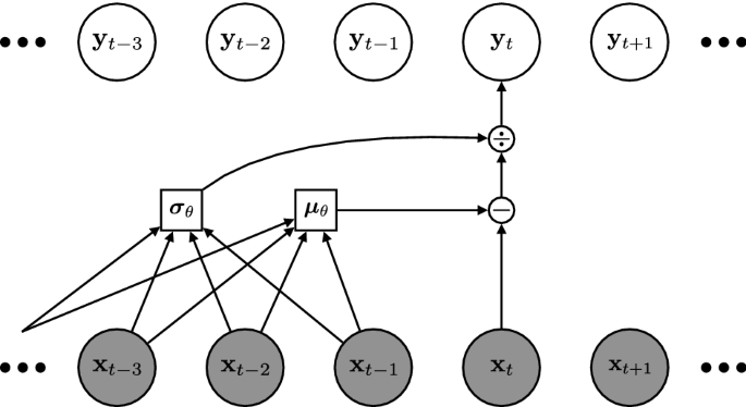
Affine autoregressive transform. Computational diagram for an affine autoregressive transform Papamakarios et al. (2017). Each \({\mathbf {y}}_t\) is an affine transform of \({\mathbf {x}}_t\), with the affine parameters potentially non-linear functions of \({\mathbf {x}}_{<t}\). The inverse transform, shown here, is capable of converting a correlated input, \({\mathbf {x}}_{1:T}\), into an uncorrelated output, \({\mathbf {y}}_{1:T}\)
2.3 Autoregressive flows
Our approach is based on affine autoregressive normalizing flows (Kingma et al. 2016; Papamakarios et al. 2017). Here, we continue with the perspective of temporal sequences, however, these flows were initially developed and demonstrated in static settings. Kingma et al. (2016) noted that sampling from an autoregressive Gaussian model is an invertible transform, resulting in a normalizing flow (Rippel and Adams 2013; Dinh et al. 2015, 2017; Rezende and Mohamed 2015). Flow-based models transform simple, base probability distributions into more complex ones while maintaining exact likelihood evaluation. To see their connection to autoregressive models, we can express sampling a Gaussian random variable using the reparameterization trick (Kingma and Welling 2014; Rezende et al. 2014):
where \({\mathbf {y}}_t \sim {\mathcal {N}} ({\mathbf {y}}_t; {\mathbf {0}}, {\mathbf {I}})\) is an auxiliary random variable and \(\odot \) denotes element-wise multiplication. Thus, \({\mathbf {x}}_t\) is an invertible transform of \({\mathbf {y}}_t\), with the inverse given as
where division is element-wise. The inverse transform in Eq. 5, shown in Fig. 2, normalizes (hence, normalizing flow) \({\mathbf {x}}_{1:T}\), removing statistical dependencies. Given the functional mapping between \({\mathbf {y}}_t\) and \({\mathbf {x}}_t\) in Eq. 4, the change of variables formula converts between probabilities in each space:
By the construction of Eqs. 4 and 5, the Jacobian in Eq. 6 is triangular, enabling efficient evaluation as the product of diagonal terms:
where i denotes the observation dimension, e.g. pixel. For a Gaussian autoregressive model, the base distribution is \(p_\theta ({\mathbf {y}}_{1:T}) = {\mathcal {N}} ({\mathbf {y}}_{1:T}; {\mathbf {0}}, {\mathbf {I}})\). We can improve upon this simple set-up by chaining transforms together, i.e. parameterizing \(p_\theta ({\mathbf {y}}_{1:T})\) as a flow, resulting in hierarchical models.
2.4 Related work
Autoregressive flows were initially considered in the contexts of variational inference (Kingma et al. 2016) and generative modeling (Papamakarios et al. 2017). These approaches are generalizations of previous approaches with affine transforms (Dinh et al. 2015, 2017). While autoregressive flows are well-suited for sequential data, these approaches, as well as many recent approaches (Huang et al. 2018; Oliva et al. 2018; Kingma and Dhariwal 2018), were initially applied to static data, such as images.
Recent works have started applying flow-based models to sequential data. van den Oord et al. (2018) and Ping et al. (2019) distill autoregressive speech models into flow-based models. Prenger et al. (2019) and Kim et al. (2019) instead train these models directly. Kumar et al. (2020) use a flow to model individual video frames, with an autoregressive prior modeling dynamics across time steps. Rhinehart et al. (2018, 2019) use autoregressive flows for modeling vehicle motion, and Henter et al. (2019) use flows for motion synthesis with motion-capture data. Ziegler and Rush (2019) model discrete observations (e.g., text) by using flows to model dynamics of continuous latent variables. Like these recent works, we apply flow-based models to sequences. However, we demonstrate that autoregressive flows can serve as a general-purpose technique for improving dynamics models. To the best of our knowledge, our work is the first to use flows to pre-process sequences to improve sequential latent variable models.
We utilize affine flows (Eq. 4), a family that includes methods like NICE (Dinh et al. 2015), RealNVP (Dinh et al. 2017), IAF (Kingma et al. 2016), MAF (Papamakarios et al. 2017), and Glow (Kingma and Dhariwal 2018). However, there has been recent work in non-affine flows (Huang et al. 2018; Jaini et al. 2019; Durkan et al. 2019), which offer further flexibility. We chose to investigate affine flows because they are commonly employed and relatively simple, however, non-affine flows could result in additional improvements.
Autoregressive dynamics models are also prominent in other related areas. Within the statistics and econometrics literature, autoregressive integrated moving average (ARIMA) is a standard technique (Box et al. 2015; Hamilton 2020), calculating differences with an autoregressive prediction to remove non-stationary components of a temporal signal. Such methods simplify downstream modeling, e.g., by removing seasonal effects. Low-level autoregressive models are also found in audio (Atal and Schroeder 1979) and video compression codecs (Wiegand et al. 2003; Agustsson et al. 2020; Yang et al. 2021), using predictive coding (Oliver 1952) to remove temporal redundancy, thereby improving downstream compression rates. Intuitively, if sequential inputs are highly predictable, it is far more efficient to compress the prediction error rather than each input (e.g., video frame) separately. Finally, we note that autoregressive models are a generic dynamics modeling approach and can, in principle, be parameterized by other techniques, such as LSTMs (Hochreiter and Schmidhuber 1997), or combined with other models, such as hidden Markov models (HMMs) (Murphy 2012).
3 Method
We now describe our approach for improving sequence modeling. First, we motivate using autoregressive flows to reduce temporal dependencies, thereby simplifying dynamics. We then show how this simple technique can be incorporated within sequential latent variable models.

Redundancy reduction. (a) Conditional densities for \(p (x_2 | x_1)\). (b) The marginal, \(p (x_2)\) differs from the conditional densities, thus, \({\mathcal {I}} (x_1 ; x_2) > 0\). (c) In the normalized space of y, the corresponding densities \(p (y_2 | y_1)\) are identical. (d) The marginal \(p(y_2)\) is identical to the conditionals, so \({\mathcal {I}} (y_1; y_2) = 0.\) Thus, in this case, a conditional affine transform removed the dependencies
3.1 Motivation: temporal redundancy reduction
Normalizing flows, while often utilized for density estimation, originated from data pre-processing techniques (Friedman 1987; Hyvärinen and Oja 2000; Chen and Gopinath 2001), which remove dependencies between dimensions, i.e., redundancy reduction (Barlow 1961). Removing dependencies simplifies the resulting probability distribution by restricting variation to individual dimensions, generally simplifying downstream tasks (Laparra et al. 2011). Normalizing flows improve upon these procedures using flexible, non-linear functions (Deco and Brauer 1995; Dinh et al. 2015). While flows have been used for spatial decorrelation (Agrawal and Dukkipati 2016; Winkler et al. 2019) and with other models (Huang et al. 2017), this capability remains under-explored.
Our main contribution is showing how to utilize autoregressive flows for temporal pre-processing to improve dynamics modeling. Data sequences contain dependencies in time, for example, in the redundancy of video pixels (Fig. 1), which are often highly predictable. These dependencies define the dynamics of the data, with the degree of dependence quantified by the multi-information,
where \({\mathcal {H}}\) denotes entropy. Normalizing flows are capable of reducing redundancy, arriving at a new sequence, \({\mathbf {y}}_{1:T}\), with \({\mathcal {I}} ({\mathbf {y}}_{1:T}) \le {\mathcal {I}} ({\mathbf {x}}_{1:T})\), thereby reducing temporal dependencies. Thus, rather than fit the data distribution directly, we can first simplify the dynamics by pre-processing sequences with a normalizing flow, then fitting the resulting sequence. Through training, the flow will attempt to remove redundancies to meet the modeling capacity of the higher-level dynamics model, \(p_\theta ({\mathbf {y}}_{1:T})\).
Example To visualize this procedure for an affine autoregressive flow, consider a one-dimensional input over two time steps, \(x_1\) and \(x_2\). For each value of \(x_1\), there is a conditional density, \(p (x_2 | x_1)\). Assume that these densities take one of two forms, which are identical but shifted and scaled, shown in Fig. 3. Transforming these densities through their conditional means, \(\mu _2 = {\mathbb {E}} \left[ x_2 | x_1 \right] \), and standard deviations, \(\sigma _2 = {\mathbb {E}} \left[ (x_2 - \mu _2)^2 | x_1 \right] ^{1/2}\), creates a normalized space, \(y_2 = (x_2 - \mu _2) / \sigma _2\), where the conditional densities are identical. In this space, the multi-information is
whereas \({\mathcal {I}} (x_1; x_2) > 0.\) Indeed, if \(p (x_t | x_{<t})\) is linear-Gaussian, inverting an affine autoregressive flow exactly corresponds to Cholesky whitening (Pourahmadi 2011; Kingma et al. 2016), removing all linear dependencies.
In the example above, \(\mu _2\) and \(\sigma _2\) act as a frame of reference for estimating \(x_2\). More generally, in the special case where \(\varvec{\mu }_\theta ({\mathbf {x}}_{<t}) = {\mathbf {x}}_{t-1}\) and \(\varvec{\sigma } ({\mathbf {x}}_{<t}) = {\mathbf {1}}\), we recover \({\mathbf {y}}_t = {\mathbf {x}}_t - {\mathbf {x}}_{t-1} = \varDelta {\mathbf {x}}_t\). Modeling finite differences (or generalized coordinates (Friston 2008)) is a well-established technique, (see, e.g. (Chua et al. 2018; Kumar et al. 2020)), which is generalized by affine autoregressive flows.

Model diagrams. a An autoregressive flow pre-processes a data sequence, \({\mathbf {x}}_{1:T}\), to produce a new sequence, \({\mathbf {y}}_{1:T}\), with reduced temporal dependencies. This simplifies dynamics modeling for a higher-level sequential latent variable model, \(p_\theta ({\mathbf {y}}_{1:T}, {\mathbf {z}}_{1:T})\). Empty diamond nodes represent deterministic dependencies, not recurrent states. b Diagram of the autoregressive flow architecture. Blank white rectangles represent convolutional layers (see Appendix). The three stacks of convolutional layers within the blue region are shared. cat denotes channel-wise concatenation
3.2 Modeling dynamics with autoregressive flows
We now discuss utilizing autoregressive flows to improve sequence modeling, highlighting use cases for modeling dynamics in the data and latent spaces.
3.2.1 Data dynamics
The form of an affine autoregressive flow across sequences is given in Eqs. 4 and 5, again, equivalent to a Gaussian autoregressive model. We can stack hierarchical chains of flows to improve the model capacity. Denoting the shift and scale functions at the \(m^\text {th}\) transform as \(\varvec{\mu }_\theta ^m (\cdot )\) and \(\varvec{\sigma }_\theta ^m (\cdot )\) respectively, we then calculate \({\mathbf {y}}^m\) using the inverse transform:
After the final (\(M^{{\text {th}}}\)) transform, we can choose the form of the base distribution, \(p_\theta ({\mathbf {y}}^M_{1:T})\), e.g. Gaussian. While we could attempt to model \({\mathbf {x}}_{1:T}\) completely using stacked autoregressive flows, these models are limited to affine element-wise transforms that maintain the data dimensionality. Due to this limited capacity, purely flow-based models often require many transforms to be effective (Kingma and Dhariwal 2018).
Instead, we can model the base distribution using an expressive sequential latent variable model (SLVM), or, equivalently, we can augment the conditional likelihood of a SLVM using autoregressive flows (Fig. 4a). Following the motivation from Sect. 3.1, the flow can remove temporal dependencies, simplifying the modeling task for the SLVM. With a single flow, the joint probability is
where the SLVM distribution is given by
If the SLVM is itself a flow-based model, we can use maximum log-likelihood training. If not, we can resort to variational inference (Chung et al. 2015; Fraccaro et al. 2016; Marino et al. 2018). We derive and discuss this procedure in the Appendix.
3.2.2 Latent dynamics
We can also consider simplifying latent dynamics modeling using autoregressive flows. This is relevant in hierarchical SLVMs, such as VideoFlow (Kumar et al. 2020), where each latent variable is modeled as a function of past and higher-level latent variables. Using \({\mathbf {z}}_t^{(\ell )}\) to denote the latent variable at the \(\ell ^{\text {th}}\) level at time t, we can parameterize the prior as
converting \({\mathbf {z}}^{(\ell )}_t\) into \({\mathbf {u}}^{(\ell )}_t\) using the inverse transform \({\mathbf {u}}^{(\ell )}_t = ({\mathbf {z}}^{(\ell )}_t - \varvec{\alpha }_\theta ({\mathbf {z}}^{(\ell )}_{<t})) / \varvec{\beta }_\theta ({\mathbf {z}}^{(\ell )}_{<t})\). As noted previously, VideoFlow uses a special case of this procedure, setting \(\varvec{\alpha }_\theta ({\mathbf {z}}^{(\ell )}_{<t}) = {\mathbf {z}}^{(\ell )}_{t-1}\) and \(\varvec{\beta }_\theta ({\mathbf {z}}^{(\ell )}_{<t}) = {\mathbf {1}}\). Generalizing this procedure further simplifies dynamics throughout the model.
4 Evaluation
We demonstrate and evaluate the proposed technique on three benchmark video datasets: Moving MNIST (Srivastava et al. 2015a), KTH Actions (Schuldt et al. 2004), and BAIR Robot Pushing (Ebert et al. 2017). In addition, we also perform experiments on several non-video sequence datasets from the UC Irvine Machine Learning Repository.Footnote 1 Specifically, we look at an activity recognition dataset (activity_rec) (Palumbo et al. 2016), an indoor localization dataset (smartphone_sensor) (Barsocchi et al. 2016), and a facial expression recognition dataset (facial_exp) (de Almeida Freitas et al. 2014). Experimental setups are described in Sect. 4.1, followed by a set of analyses in Sect. 4.2. Further details and results can be found in the Appendix.

Decreased temporal correlation. a Affine autoregressive flows result in sequences, \({\mathbf {y}}_{1:T}\), with decreased temporal correlation, \(\text {corr}_{\mathbf {y}}\), as compared with that of the original data, \(\text {corr}_{\mathbf {x}}\). The presence of a more powerful base distribution (SLVM) reduces the need for decorrelation. Additional flow transforms further decrease correlation (note: \(|\text {corr}_{\mathbf {y}}| < 0.01\) for 2-AF). (b) For SLVM + 1-AF, \(\text {corr}_{\mathbf {y}}\) decreases during training on KTH Actions (Color figure online)
4.1 Experimental setup
We empirically evaluate the improvements to downstream dynamics modeling from temporal pre-processing via autoregressive flows. For data space modeling, we compare four model classes: (1) standalone affine autoregressive flows with one (1-AF) and (2) two (2-AF) transforms, (3) a sequential latent variable model (SLVM), and (4) SLVM with flow-based pre-processing (SLVM + 1-AF). As we are not proposing a specific architecture, but rather a general modeling technique, the SLVM architecture is representative of recurrent convolutional video models with a single latent level (Denton and Fergus 2018; Ha and Schmidhuber 2018; Hafner et al. 2019). Flows are implemented with convolutional networks, taking in a fixed window of previous frames (Fig. 4b). These models allow us to evaluate the benefits of temporal pre-processing (SLVM vs. SLVM + 1-AF) and the benefits of more expressive higher-level dynamics models (2-AF vs. SLVM + 1-AF).
To evaluate latent dynamics modeling with flows, we use the tensor2tensor library (Vaswani et al. 2018) to compare (1) VideoFlowFootnote 2 and (2) the same model with affine autoregressive flow latent dynamics (VideoFlow + AF). VideoFlow is significantly larger (\(3\times \) more parameters) than the one-level SLVM, allowing us to evaluate whether autoregressive flows are beneficial in this high-capacity regime.
To enable a fairer comparison in our experiments, models with autoregressive flow dynamics have comparable or fewer parameters than baseline counterparts. We note that autoregressive dynamics adds only a constant computational cost per time-step, and this computation can be parallelized for training and evaluation. Full architecture, training, and analysis details can be found in the Appendix. Finally, as noted by Kumar et al. (2020), many previous works do not train SLVMs with proper log-likelihood objectives. Our SLVM results are consistent with previously reported log-likelihood values (Marino et al. 2018) for the Stochastic Video Generation model (Denton and Fergus 2018) trained with a log-likelihood bound objective.

Flow Visualization for SLVM + 1-AF on Moving MNIST (left) and KTH Actions (right)

Improved Generated Samples. Random samples generated from (a) VideoFlow and (b) VideoFlow + AF, each conditioned on the first 3 frames. Using AF produces more coherent samples. The robot arm blurs for VideoFlow in samples 1 and 4 (red boxes), but does not blur for VideoFlow + AF (Color figure online)
4.2 Analyses
Visualization In Fig. 1, we visualize the pre-processing procedure for SLVM + 1-AF on BAIR Robot Pushing. The plots show the RGB values for a pixel before (top) and after (bottom) the transform. The noise sequence is nearly zero throughout, despite large changes in the pixel value. We also see that the noise sequence (center, lower) is invariant to the static background, capturing the moving robotic arm. At some time steps (e.g. fourth frame), the autoregressive flow incorrectly predicts the next frame, however, the higher-level SLVM compensates for this prediction error.
We also visualize each component of the flow. Figure 4b illustrates this for SLVM + 1-AF on an input from BAIR Robot Pushing. We see that \(\varvec{\mu }_\theta \) captures the static background, while \(\varvec{\sigma }_\theta \) highlights regions of uncertainty. In Fig. 6 and the Appendix, we present visualizations on full sequences, where we see that different models remove varying degrees of temporal structure.
Temporal Redundancy Reduction To quantify temporal redundancy reduction, we evaluate the empirical correlation (linear dependence) between frames, denoted as corr, for the data and noise variables. We evaluate \(\text {corr}_{{\mathbf {x}}}\) and \(\text {corr}_{{\mathbf {y}}}\) for 1-AF, 2-AF, and SLVM + 1-AF. The results are shown in Fig. 5a. In Fig. 5b, we plot \(\text {corr}_{{\mathbf {y}}}\) for SLVM + 1-AF during training on KTH Actions. Flows decrease temporal correlation, with additional transforms yielding further decorrelation. Base distributions without temporal structure (1-AF) yield comparatively more decorrelation. Temporal redundancy is progressively removed throughout training. Note that 2-AF almost completely removes temporal correlations (\(|\text {corr}_{\mathbf {y}}| < 0.01\)). However, note that this only quantifies linear dependencies, and more complex non-linear dependencies may require the use of higher-level dynamics models, as shown through quantitative comparisons.
Performance Comparison Table 1 reports average test negative log-likelihood results on video datasets. Standalone flow-based models perform surprisingly well. Increasing flow depth from 1-AF to 2-AF generally results in improvement. SLVM + 1-AF outperforms the baseline SLVM despite having fewer parameters. As another baseline, we also consider modeling frame differences, \(\varDelta {\mathbf {x}} \equiv {\mathbf {x}}_t - {\mathbf {x}}_{t-1}\), with SLVM, which can be seen as a special case of 1-AF with \(\varvec{\mu }_\theta = {\mathbf {x}}_{t-1}\) and \(\varvec{\sigma }_\theta = {\mathbf {1}}\). On BAIR and KTH Actions, datasets with significant temporal redundancy (Fig. 5a), this technique improves performance over SLVM. However, on Moving MNIST, modeling \(\varDelta {\mathbf {x}}\) actually decreases performance, presumably by creating more complex spatial patterns. In all cases, the learned temporal transform, SLVM + 1-AF, outperforms this hard-coded transform, SLVM + \(\varDelta {\mathbf {x}}\). Finally, incorporating autoregressive flows into VideoFlow results in a modest but noticeable improvement, demonstrating that removing spatial dependencies, through VideoFlow, and temporal dependencies, through autoregressive flows, are complementary techniques.

Improved Generalization. The low-level reference frame improves generalization to unseen sequences. Train and test negative log-likelihood bound histograms for (a) SLVM and (b) SLVM + 1-AF on KTH Actions. (c) The generalization gap for SLVM + 1-AF remains small for varying amounts of KTH training data, while it becomes worse in the low-data regime for SLVM (Color figure online)
Results on Non-Video Sequence Dataset In Table 2, we report negative log-density results on non-video data in nats per time step. Note that log-densities can be positive or negative. Again, we see that 2-AF consistently outperforms 1-AF, which are typically on-par or better than SLVM. However, SLVM + 1-AF outperforms all other model classes, achieving the lowest (best) log-densities across all datasets. With non-video data, we see that using the special case of modeling temporal differences (SLVM + \(\varDelta {\mathbf {x}}\)), performance is actually slightly worse than that of SLVM on all datasets. This, again, highlights the importance of using a learned pre-processing transform in comparison with hard-coded temporal differences.
Improved Samples The quantitative improvement over VideoFlow is less dramatic, as this is already a high-capacity model. However, qualitatively, we observe that incorporating autoregressive flow dynamics improves sample quality (Fig. 7). In these randomly selected samples, the robot arm occasionally becomes blurry for VideoFlow (red boxes) but remains clear for VideoFlow + AF.
Improved Generalization Our temporal normalization technique also improves generalization to unseen examples, a key benefit of normalization schemes, e.g., batch norm (Ioffe and Szegedy 2015). Intuitively, higher-level dynamics are often preserved, whereas lower-level appearance is not. This is apparent on KTH Actions, which contains a substantial degree of train-test mismatch, due to different identities and activities. NLL histograms on KTH are shown in Fig. 8, with greater overlap for SLVM + 1-AF. We also train SLVM and SLVM + 1-AF on subsets of KTH Actions. In Fig. 8c, we see that autoregressive flows enable generalization in the low-data regime, whereas SLVM becomes worse.
5 Conclusion
We have presented a technique for improving sequence modeling using autoregressive flows. Learning a frame of reference, parameterized by autoregressive transforms, reduces temporal redundancy in input sequences, simplifying dynamics. Thus, rather than expanding the model, we can simplify the input to meet the capacity of the model. This approach is distinct from previous works with normalizing flows on sequences, yet contains connections to classical modeling and compression. We hope these connections lead to further insights and applications. Finally, we have analyzed and empirically shown how autoregressive pre-processing in both the data and latent spaces can improve sequence modeling and lead to improved sample quality and generalization.
The underlying assumption behind using autoregressive flows for sequence modeling is that sequences contain smooth or predictable temporal dependencies, with more complex, higher-level dependencies as well. In both video and non-video data, we have seen improvements from combining sequential latent variable models with autoregressive flows, suggesting that such assumptions are generally reasonable. Using affine autoregressive flows restricts our approach to sequences of continuous data, but future work could investigate discrete data, such as natural language. Likewise, we assume regularly sampled sequences (i.e., a constant frequency), however, future work could also investigate irregularly sampled event data.
Notes
We used a smaller version of the original model architecture, with half of the flow depth, due to GPU memory constraints.
References
Agrawal, S., & Dukkipati, A. (2016). Deep variational inference without pixel-wise reconstruction. arXiv preprint arXiv:161105209
Agustsson, E., Minnen, D., Johnston, N., Balle, J., Hwang, S. J., & Toderici, G. (2020). Scale-space flow for end-to-end optimized video compression. In Proceedings of the IEEE/CVF Conference on Computer Vision and Pattern Recognition (pp. 8503–8512).
de Almeida Freitas, F., Peres, S. M., de Moraes Lima, C. A., & Barbosa, F. V. (2014). Grammatical facial expressions recognition with machine learning. In The Twenty-Seventh International Flairs Conference.
Atal, B., & Schroeder, M. (1979). Predictive coding of speech signals and subjective error criteria. IEEE Transactions on Acoustics, Speech, and Signal Processing, 27(3), 247–254.
Barlow, H. B., et al. (1961). Possible principles underlying the transformation of sensory messages. Sensory communication, 1, 217–234.
Barsocchi, P., Crivello, A., La Rosa, D., & Palumbo, F. (2016). A multisource and multivariate dataset for indoor localization methods based on wlan and geo-magnetic field fingerprinting. In 2016 International Conference on Indoor Positioning and Indoor Navigation (IPIN) (pp 1–8). IEEE.
Bayer, J., & Osendorfer, C. (2014). Learning stochastic recurrent networks. In NeurIPS 2014 Workshop on Advances in Variational Inference.
Bengio, Y., & Bengio, S. (2000). Modeling high-dimensional discrete data with multi-layer neural networks. In Advances in Neural Information Processing Systems (pp. 400–406).
Box, G. E., Jenkins, G. M., Reinsel, G. C., & Ljung, G. M. (2015). Time series analysis: forecasting and control. Wiley.
Chen, S. S., & Gopinath, R. A. (2001). Gaussianization. In Advances in Neural Information Processing Systems (pp. 423–429).
Chua, K., Calandra, R., McAllister, R., & Levine, S. (2018). Deep reinforcement learning in a handful of trials using probabilistic dynamics models. In Advances in Neural Information Processing Systems (pp. 4754–4765).
Chung, J., Kastner, K., Dinh, L., Goel, K., Courville, A. C., & Bengio, Y. (2015). A recurrent latent variable model for sequential data. In Advances in Neural Information processing Systems (pp. 2980–2988).
Clevert, D. A., Unterthiner, T., & Hochreiter, S. (2015). Fast and accurate deep network learning by exponential linear units (elus). arXiv preprint arXiv:151107289
Deco, G., & Brauer, W. (1995). Higher order statistical decorrelation without information loss. In Advances in Neural Information Processing Systems (pp. 247–254)
Denton, E., & Fergus, R. (2018). Stochastic video generation with a learned prior. In International Conference on Machine Learning (pp. 1182–1191).
Dinh, L., Krueger, D., & Bengio, Y. (2015). Nice: Non-linear independent components estimation. In International Conference on Learning Representations.
Dinh, L., Sohl-Dickstein, J., & Bengio, S. (2017). Density estimation using real nvp. In International Conference on Learning Representations.
Durkan, C., Bekasov, A., Murray, I., & Papamakarios, G. (2019). Neural spline flows. In Advances in Neural Information Processing Systems.
Ebert, F., Finn, C., Lee, A. X., & Levine, S. (2017). Self-supervised visual planning with temporal skip connections. In Conference on Robot Learning.
Fraccaro, M., Sønderby, S. K., Paquet, U., & Winther, O. (2016). Sequential neural models with stochastic layers. In Advances in Neural Information Processing Systems (pp. 2199–2207).
Frey, B. J., Hinton, G. E., & Dayan, P. (1996). Does the wake-sleep algorithm produce good density estimators? In Advances in Neural Information Processing Systems (pp. 661–667).
Friedman, J. H. (1987). Exploratory projection pursuit. Journal of the American statistical association, 82(397), 249–266.
Friston, K. (2008). Hierarchical models in the brain. PLoS Computational Biology, 4(11), e1000211.
Gan, Z., Li, C., Henao, R., Carlson, D. E., & Carin, L. (2015). Deep temporal sigmoid belief networks for sequence modeling. In Advances in Neural Information Processing Systems.
Gemici, M., Hung, C. C., Santoro, A., Wayne, G., Mohamed, S., Rezende, D. J., Amos, D., & Lillicrap, T. (2017) .Generative temporal models with memory. arXiv preprint arXiv:170204649
Graves, A. (2013). Generating sequences with recurrent neural networks. arXiv preprint arXiv:13080850
Ha, D., & Schmidhuber, J. (2018). Recurrent world models facilitate policy evolution. In Advances in Neural Information Processing Systems (pp. 2450–2462).
Hafner, D., Lillicrap, T., Fischer, I., Villegas, R., Ha, D., Lee, H., & Davidson, J. (2019). Learning latent dynamics for planning from pixels. In International Conference on Machine Learning (pp. 2555–2565).
Hamilton, J. D. (2020). Time series analysis. Princeton University Press.
He, J., Lehrmann, A., Marino, J., Mori, G., & Sigal, L. (2018). Probabilistic video generation using holistic attribute control. In Proceedings of the European Conference on Computer Vision (ECCV) (pp. 452–467).
Henter, G. E., Alexanderson, S., & Beskow, J. (2019). Moglow: Probabilistic and controllable motion synthesis using normalising flows. arXiv preprint arXiv:190506598
Hochreiter, S., & Schmidhuber, J. (1997). Long short-term memory. Neural Computation, 9(8), 1735–1780.
Huang, C. W., Touati, A., Dinh, L., Drozdzal, M., Havaei, M., Charlin, L., & Courville, A. (2017). Learnable explicit density for continuous latent space and variational inference. arXiv preprint arXiv:171002248
Huang, C. W., Krueger, D., Lacoste, A., & Courville, A. (2018) Neural autoregressive flows. In International Conference on Machine Learning (pp. 2083–2092).
Hyvärinen, A., & Oja, E. (2000). Independent component analysis: Algorithms and applications. Neural Networks, 13(4–5), 411–430.
Ioffe, S., & Szegedy, C. (2015). Batch normalization: Accelerating deep network training by reducing internal covariate shift. In International Conference on Machine Learning (pp. 448–456).
Jaini, P., Selby, K. A., & Yu, Y. (2019). Sum-of-squares polynomial flow. In International Conference on Machine Learning (pp. 3009–3018).
Jordan, M. I., Ghahramani, Z., Jaakkola, T. S., & Saul, L. K. (1998). An introduction to variational methods for graphical models. Nato Asi Series D Behavioural And Social Sciences, 89, 105–162.
Karl, M., Soelch, M., Bayer, J., van der Smagt, P. (2017). Deep variational bayes filters: Unsupervised learning of state space models from raw data. In International Conference on Learning Representations.
Kim, S., Lee, S. G., Song, J., Kim, J., & Yoon, S. (2019). Flowavenet: A generative flow for raw audio. In International Conference on Machine Learning (pp. 3370–3378).
Kingma, D. P., & Ba, J. (2015). Adam: A method for stochastic optimization. In International Conference on Learning Representations.
Kingma, D. P., & Dhariwal, P. (2018). Glow: Generative flow with invertible 1x1 convolutions. In Advances in Neural Information Processing Systems (pp. 10215–10224).
Kingma, D. P., & Welling, M. (2014). Stochastic gradient vb and the variational auto-encoder. In Proceedings of the International Conference on Learning Representations.
Kingma, D. P., Salimans, T., Jozefowicz, R., Chen, X., Sutskever, I., & Welling, M. (2016). Improved variational inference with inverse autoregressive flow. In Advances in Neural Information Processing Systems (pp. 4743–4751).
Kumar, M., Babaeizadeh, M., Erhan, D., Finn, C., Levine, S., Dinh, L., & Kingma, D. (2020). Videoflow: A flow-based generative model for video. In International Conference on Learning Representations.
Laparra, V., Camps-Valls, G., & Malo, J. (2011). Iterative gaussianization: from ica to random rotations. IEEE transactions on neural networks, 22(4), 537–549.
Li, Y., & Mandt, S. (2018). A deep generative model for disentangled representations of sequential data. In International Conference on Machine Learning.
Lombardo, S., Han, J., Schroers, C., & Mandt, S. (2019). Deep generative video compression. In Advances in Neural Information Processing Systems (pp. 9283–9294).
Marino, J., Cvitkovic, M., & Yue, Y. (2018). A general method for amortizing variational filtering. In Advances in Neural Information Processing Systems (pp. 7857–7868).
Murphy, K. P. (2012). Machine learning: a probabilistic perspective. MIT press.
Oliva, J., Dubey, A., Zaheer, M., Poczos, B., Salakhutdinov, R., Xing, E., & Schneider, J. (2018). Transformation autoregressive networks. In International Conference on Machine Learning (pp. 3895–3904).
Oliver, B. (1952). Efficient coding. The Bell System Technical Journal, 31(4), 724–750.
van den Oord, A., Dieleman, S., Zen, H., Simonyan, K., Vinyals, O., Graves, A., Kalchbrenner, N., Senior, A., & Kavukcuoglu, K. (2016a). Wavenet: A generative model for raw audio. arXiv preprint arXiv:160903499
van den Oord, A., Kalchbrenner, N., & Kavukcuoglu, K. (2016b). Pixel recurrent neural networks. In International Conference on Machine Learning (pp. 1747–1756).
van den Oord, A., Li, Y., Babuschkin, I., Simonyan, K., Vinyals, O., Kavukcuoglu, K., Driessche, G., Lockhart, E., Cobo, L., Stimberg, F., et al. (2018). Parallel wavenet: Fast high-fidelity speech synthesis. In International Conference on Machine Learning (pp. 3915–3923).
Palumbo, F., Gallicchio, C., Pucci, R., & Micheli, A. (2016). Human activity recognition using multisensor data fusion based on reservoir computing. Journal of Ambient Intelligence and Smart Environments, 8(2), 87–107.
Papamakarios, G., Pavlakou, T., & Murray, I. (2017). Masked autoregressive flow for density estimation. In Advances in Neural Information Processing Systems (pp. 2338–2347).
Ping, W., Peng, K., & Chen, J. (2019). Clarinet: Parallel wave generation in end-to-end text-to-speech. In International Conference on Learning Representations.
Pourahmadi, M. (2011). Covariance estimation: The glm and regularization perspectives. Statistical Science (pp. 369–387).
Prenger, R., Valle, R., & Catanzaro, B. (2019). Waveglow: A flow-based generative network for speech synthesis. ICASSP 2019–2019 IEEE International Conference on Acoustics, Speech and Signal Processing (ICASSP) (pp. 3617–3621). IEEE.
Radford, A., Metz, L., & Chintala, S. (2015). Unsupervised representation learning with deep convolutional generative adversarial networks. arXiv preprint arXiv:151106434
Rezende, D., & Mohamed, S. (2015). Variational inference with normalizing flows. In International Conference on Machine Learning (pp. 1530–1538).
Rezende, D. J., Mohamed, S., & Wierstra, D. (2014). Stochastic backpropagation and approximate inference in deep generative models. In Proceedings of the International Conference on Machine Learning (pp. 1278–1286).
Rhinehart, N., Kitani, K. M., & Vernaza, P. (2018) R2p2: A reparameterized pushforward policy for diverse, precise generative path forecasting. In Proceedings of the European Conference on Computer Vision (ECCV) (pp. 772–788).
Rhinehart, N., McAllister, R., Kitani, K., & Levine, S. (2019). Precog: Prediction conditioned on goals in visual multi-agent settings. In Proceedings of the International Conference on Computer Vision (ICCV).
Rippel, O., & Adams, R. P. (2013). High-dimensional probability estimation with deep density models. arXiv preprint arXiv:13025125
Schmidt, F., Mandt, S., & Hofmann, T. (2019). Autoregressive text generation beyond feedback loops. In Empirical Methods in Natural Language Processing (pp. 3391–3397).
Schuldt, C., Laptev, I., & Caputo, B. (2004). Recognizing human actions: A local svm approach. In International Conference on Pattern Recognition.
Srinivasan, M. V., Laughlin, S. B., & Dubs, A. (1982). Predictive coding: A fresh view of inhibition in the retina. Proceedings of the Royal Society of London Series B Biological Sciences, 216(1205), 427–459.
Srivastava, N., Mansimov, E., & Salakhudinov, R. (2015a). Unsupervised learning of video representations using lstms. In International conference on Machine Learning (pp. 843–852).
Srivastava, R. K., Greff, K., & Schmidhuber, J. (2015b). Training very deep networks. In Advances in neural information processing systems (NIPS) (pp. 2377–2385).
Vaswani, A., Bengio, S., Brevdo, E., Chollet, F., Gomez, A. N., Gouws, S., Jones, L., Kaiser, L., Kalchbrenner, N., Parmar, N., Sepassi, R., Shazeer, N., & Uszkoreit, J. (2018). Tensor2tensor for neural machine translation. CoRR abs/1803.07416, arXiv:1803.07416
Wiegand, T., Sullivan, G. J., Bjontegaard, G., & Luthra, A. (2003). Overview of the h. 264/avc video coding standard. IEEE Transactions on circuits and systems for video technology, 13(7), 560–576.
Winkler, C., Worrall, D., Hoogeboom, E., & Welling, M. (2019). Learning likelihoods with conditional normalizing flows. arXiv preprint arXiv:191200042
Xue, T., Wu, J., Bouman, K., & Freeman, B. (2016). Visual dynamics: Probabilistic future frame synthesis via cross convolutional networks. In Advances in Neural Information Processing Systems.
Yang, R., Yang, Y., Marino, J., & Mandt, S. (2021). Hierarchical autoregressive modeling for neural video compression. In International Conference on Learning Representations.
Ziegler, Z., & Rush, A. (2019) Latent normalizing flows for discrete sequences. In International Conference on Machine Learning (pp. 7673–7682).
Author information
Authors and Affiliations
Contributions
Joseph Marino: forming idea, running simulation and writing paper; Lei Chen: running simulation; Jiawei He: writing paper, and Stephan Mandt: forming idea, writing paper and providing feedback. All authors worked toegther for most of the ta sks involved.
Corresponding author
Ethics declarations
Conflict of interest
California Institute of Technology (caltech.edu); Simon Fraser University (sfu.ca); University of California Irvine (uci.edu); Disney Research (disneyresearch.com); Borealis AI (borealisai.com); DeepMind (deepmind.com, google.com)
Code availability
Source code is available at https://anonymous.4open.science/r/f02199f7-86d2-45ee-ad23-3f13f769ee10/.
Additional information
Publisher's Note
Springer Nature remains neutral with regard to jurisdictional claims in published maps and institutional affiliations.
Editor: Gustavo Batista.
Appendices
Appendix A: Lower bound derivation
Consider the model defined in Sect. 3.3, with the conditional likelihood parameterized with autoregressive flows. That is, we parameterize
yielding
The joint distribution over all time steps is then given as
To perform variational inference, we consider a filtering approximate posterior of the form
We can then plug these expressions into the evidence lower bound:
Finally, in the filtering setting, we can rewrite the expectation, bringing it inside of the sum (see Gemici et al. 2017; Marino et al. 2018):
Because there exists a one-to-one mapping between \({\mathbf {x}}_{1:T}\) and \({\mathbf {y}}_{1:T}\), we can equivalently condition the approximate posterior and the prior on \({\mathbf {y}}\), i.e.
Appendix B: Experiment details
1.1 Flow architecture
The affine autoregressive flow architecture is shown in Fig. 9. The shift and scale of the affine transform are conditioned on three previous inputs. For each flow, we first apply 4 convolutional layers with kernel size (3, 3), stride 1, and padding 1 on each conditioned observation, preserving the input shape. The outputs are concatenated along the channel dimension and go through another 4 convolutional layers with kernel size (3, 3), stride 1, and padding 1. Finally, separate convolutional layers with the same kernel size, stride, and padding are used to output shift and log-scale. We use ReLU non-linearities for all convolutional layers.
1.2 Sequential latent variable model architecture
For sequential latent variable models, we use a DC-GAN (Radford et al. 2015) encoder architecture (Fig. 9d), with 4 convolutional layers of kernel size (4, 4), stride 2, and padding 1 followed by another convolutional layer of kernel size (4, 4), stride 1, and no padding. The encoding is sent to one or two LSTM layers (Hochreiter and Schmidhuber 1997) followed by separate linear layers to output the mean and log-variance for \(q_\phi ({\mathbf {z}}_t | {\mathbf {x}}_{\le t}, {\mathbf {z}}_{<t})\). We note that for SLVM, we input \({\mathbf {x}}_t\) into the encoder, whereas for SLVM + AF, we input \({\mathbf {y}}_t\). The architecture for the conditional prior, \(p_\theta ({\mathbf {z}}_t | {\mathbf {x}}_{<t}, {\mathbf {z}}_{<t})\), shown in Fig. 9e, contains two fully-connected layers, which take the previous latent variable as input, followed by one or two LSTM layers, and separate linear layers to output the mean and log-variance. The decoder architecture, shown in Fig. 9c, mirrors the encoder architecture, using transposed convolutions. In SLVM, we use two LSTM layers for modeling the conditional prior and approximate posterior distributions, while in SLVM + 1-AF, we use a single LSTM layer for each. We use leaky ReLU non-linearities for the encoder and decoder architectures and ReLU non-linearities in the conditional prior architecture.
1.3 Videoflow architecture
For VideoFlow experiments, we use the official code provided by Kumar et al. (2020) in the tensor2tensor repository (Vaswani et al. 2018). Due to memory and computational constraints, we use a smaller version of the model architecture used by Kumar et al. (2020) for the BAIR Robot Pushing dataset. We change depth from 24 to 12 and latent_encoder_width from 256 to 128. This reduces the number of parameters from roughly 67 million to roughly 32 million. VideoFlow contains a hierarchy of latent variables, with the latent variable at level l at time t denoted as \({\mathbf {z}}_t^{(l)}\). The prior on this latent variable is denoted as \(p_\theta ({\mathbf {z}}_t^{(l)} | {\mathbf {z}}_{<t}^{(l)}, {\mathbf {z}}_t^{(>l)}) = {\mathcal {N}} ({\mathbf {z}}_t^{(l)}; \varvec{\mu }_t^{(l)}, \text {diag} ((\varvec{\sigma }_t^{(l)})^2))\), where \(\varvec{\mu }_t^{(l)}\) and \(\varvec{\sigma }_t^{(l)}\) are functions of \({\mathbf {z}}_{<t}^{(l)}\) and \({\mathbf {z}}_t^{(>l)}\). We note that Kumar et al. (2020) parameterize \(\varvec{\mu }_t^{(l)}\) as \(\varvec{\mu }_t^{(l)} = {\mathbf {z}}_{t-1}^{(l)} + \widetilde{\varvec{\mu }}_t^{(l)}\), where \(\widetilde{\varvec{\mu }}_t^{(l)}\) is the function. Kumar et al. (2020) refer to this as latent_skip. This is already a special case of an affine autoregressive flow, with a hard-coded shift of \({\mathbf {z}}_{t-1}^{(l)}\) and a scale of \({\mathbf {1}}\). We parameterize an affine autoregressive flow at each latent level, with a shift, \(\varvec{\alpha }_t^{(l)}\), and scale, \(\varvec{\beta }_t^{(l)}\), which are function of \({\mathbf {z}}_{<t}^{(l)}\), using the same 5-block ResNet architecture as Kumar et al. (2020). In practice, these functions are conditioned on the variables at the past three time steps. The affine autoregressive flow produces a new variable:
which we then model using the same prior distribution and architecture as Kumar et al. (2020): \(p_\theta ({\mathbf {u}}_t^{(l)} | {\mathbf {z}}_{<t}^{(l)}, {\mathbf {z}}_t^{(>l)}) = {\mathcal {N}} ({\mathbf {u}}_t^{(l)}; \varvec{\mu }_t^{(l)}, \text {diag} ((\varvec{\sigma }_t^{(l)})^2))\), where \(\varvec{\mu }_t^{(l)}\) and \(\varvec{\sigma }_t^{(l)}\), again, are functions of \({\mathbf {z}}_{<t}^{(l)}\) (or, equivalently \({\mathbf {u}}_{<t}^{(l)}\)) and \({\mathbf {z}}_t^{(>l)}\).
1.4 Non-video sequence modeling architecture
We again compare various model classes in terms of log-likelihood estimation. We use fully-connected networks to parameterize all functions within the prior, approximate posterior, and conditional likelihood of each model. All networks are 2 layers of 256 units with highway connectivity (Srivastava et al. 2015b). For autoregressive flows, we use ELU non-linearities (Clevert et al. 2015). For stability, we found it necessary to use tanh non-linearities in the networks for SLVMs (prior, conditional likelihood, and approximate posterior). In SLVMs, the prior is conditioned on \({\mathbf {z}}_{t-1}\), the approximate posterior is conditioned on \({\mathbf {z}}_{t-1}\) and \({\mathbf {y}}_{t}\), and the conditional likelihood is conditioned on \({\mathbf {z}}_t\). We use a latent space dimensionality of 16 for all SLVMs.
1.5 Training set-up
We use the Adam optimizer Kingma and Ba (2015) with a learning rate of \(1 \times 10^{-4}\) to train all the models. For Moving MNIST, we use a batch size of 16 and train for 200, 000 iterations for SLVM and 100, 000 iterations for 1-AF, 2-AF and SLVM + 1-AF. For BAIR Robot Pushing, we use a batch size of 8 and train for 200, 000 iterations for all models. For KTH Actions, we use a batch size of 8 and train for 90, 000 iterations for all models. Batch norm (Ioffe and Szegedy 2015) is applied to all convolutional layers that do not output distribution or affine transform parameters. We randomly crop sequences of length 13 from all sequences and evaluate on the last 10 frames. For AF-2 models, we crop sequences of length 16 in order to condition both flows on three previous inputs. For VideoFlow experiments, we use the same hyper-parameters as Kumar et al. (2020) (with the exception of the two architecture changes mentioned above) and train for 100, 000 iterations (Table 3).
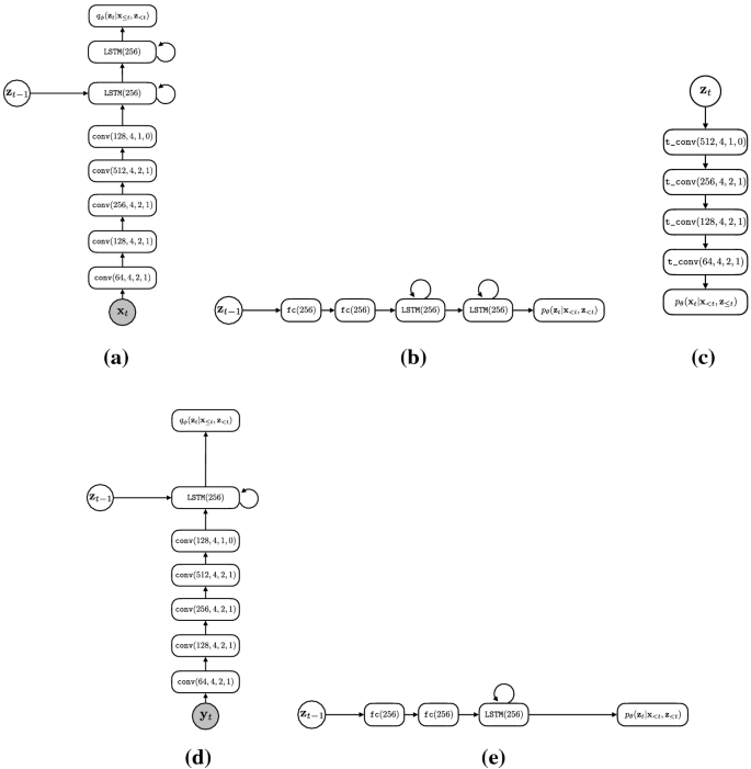
SLVM Architecture. Diagrams are shown for the (a) approximate posterior, (b) prior, and (c) conditional likelihood of the sequential latent variable model (SLVM). In (d) and (e) we show the approximate posterior and prior used with SLVM + AF, respectively. The conditional likelihood is the same architecture in both setups. Note: for SLVM + AF, we input \({\mathbf {y}}_t\) into the approximate posterior encoder, rather than \({\mathbf {x}}_t\). conv denotes a convolutional layer, LSTM denotes a long short-term memory layer, fc denotes a fully-connected layer, and t_conv denotes a transposed convolutional layer. For conv and t_conv layers, the numbers in parentheses respectively denote the number of filters, filter size, stride, and padding of the layer. For fc and LSTM layers, the number in parentheses denotes the number of units. SLVM contains one additional LSTM layer in both the approximate posterior and conditional prior
1.6 Quantifying decorrelation
To quantify the temporal redundancy reduction resulting from affine autoregressive pre-processing, we evaluate the empirical correlation between successive frames for the data observations and noise variables, averaged over spatial locations and channels. This is an average normalized version of the auto-covariance of each signal with a time delay of 1 time step. Specifically, we estimate the temporal correlation as
where the term inside the expectation is
Here, \(x_t^{(i, j, k)}\) denotes the image at location (i, j) and channel k at time t, \(\mu ^{(i, j, k)}\) is the mean of this dimension, and \(\sigma ^{(i, j, k)}\) is the standard deviation. H, W, and C respectively denote the height, width, and number of channels of the observations, and \({\mathcal {D}}\) denotes the dataset. We define an analogous expression for \({\mathbf {y}}\), denoted \(\text {corr}_{{\mathbf {y}}}\).
Appendix C: Illustrative example
To build intuition behind the benefits of temporal pre-processing (e.g., decorrelation) for downstream dynamics modeling, we present the following simple, kinematic example. Consider the discrete dynamical system defined by the following set of equations:
where \({\mathbf {w}}_t \sim {\mathcal {N}} ({\mathbf {w}}_t; {\mathbf {0}}, \varvec{\varSigma })\). We can express \({\mathbf {x}}_t\) and \({\mathbf {u}}_t\) in probabilistic terms as
Physically, this describes the noisy dynamics of a particle with momentum and mass 1, subject to Gaussian noise. That is, \({\mathbf {x}}\) represents position, \({\mathbf {u}}\) represents velocity, and \({\mathbf {w}}\) represents stochastic forces. If we consider the dynamics at the level of \({\mathbf {x}}\), we can use the fact that \({\mathbf {u}}_{t-1} = {\mathbf {x}}_{t-1} - {\mathbf {x}}_{t-2}\) to write
Thus, we see that in the space of \({\mathbf {x}}\), the dynamics are second-order Markov, requiring knowledge of the past two time steps. However, at the level of \({\mathbf {u}}\) (Eq. 28), the dynamics are first-order Markov, requiring only the previous time step. Yet, note that \({\mathbf {u}}_t\) is, in fact, an affine autoregressive transform of \({\mathbf {x}}_t\) because \({\mathbf {u}}_t = {\mathbf {x}}_t - {\mathbf {x}}_{t-1}\) is a special case of the general form \(\frac{{\mathbf {x}}_t - \varvec{\mu }_\theta ({\mathbf {x}}_{<t})}{\varvec{\sigma }_\theta ({\mathbf {x}}_{<t})}\). In Eq. 25, we see that the Jacobian of this transform is \(\partial {\mathbf {x}}_t / \partial {\mathbf {u}}_t = {\mathbf {I}}\), so, from the change of variables formula, we have \(p ({\mathbf {x}}_t | {\mathbf {x}}_{t-1}, {\mathbf {x}}_{t-2}) = p ({\mathbf {u}}_t | {\mathbf {u}}_{t-1})\). In other words, an affine autoregressive transform has allowed us to convert a second-order Markov system into a first-order Markov system, thereby simplifying the dynamics. Continuing this process to move to \({\mathbf {w}}_t = {\mathbf {u}}_t - {\mathbf {u}}_{t-1}\), we arrive at a representation that is entirely temporally decorrelated, i.e. no dynamics, because \(p ({\mathbf {w}}_t) = {\mathcal {N}} ({\mathbf {w}}_t; {\mathbf {0}}, \varvec{\varSigma })\). A sample from this system is shown in Fig. 10, illustrating this process of temporal decorrelation (Table 4) (Figs 11, 12, 13 and 14).

Motivating example. Plots are shown for a sample of \({\mathbf {x}}_{1:T}\) (left), \({\mathbf {u}}_{1:T}\) (center), and \({\mathbf {w}}_{1:T}\) (right). Here, \({\mathbf {w}}_{1:T} \sim {\mathcal {N}} ({\mathbf {w}}_{1:T}; {\mathbf {0}}, {\mathbf {I}})\), and \({\mathbf {u}}\) and \({\mathbf {x}}\) are initialized at 0. Moving from \({\mathbf {x}} \rightarrow {\mathbf {u}} \rightarrow {\mathbf {w}}\) via affine transforms results in successively less temporal correlation and therefore simpler dynamics
Appendix D: Additional experimental results
1.1 Additional qualitative results

Autoregressive Flow Visualization on KTH Action. Visualization of the flow component for (a) standalone flow-based models and (b) sequential latent variable models with flow-based conditional likelihoods for KTH Actions. From top to bottom, each figure shows (1) the original frames, \({\mathbf {x}}_t\), (2) the predicted shift, \(\varvec{\mu }_\theta ({\mathbf {x}}_{<t})\), for the frame, (3) the predicted scale, \(\varvec{\sigma }_\theta ({\mathbf {x}}_{<t})\), for the frame, and (4) the noise, \({\mathbf {y}}_t\), obtained from the inverse transform

SLVM w/ 2-AF Visualization on Moving MNIST. Visualization of the flow component for sequential latent variable models with 2-layer flow-based conditional likelihoods for Moving MNIST. From top to bottom on the left side, each figure shows (1) the original frames, \({\mathbf {x}}_t\), (2) the lower-level predicted shift, \(\varvec{\mu }_\theta ^1 ({\mathbf {x}}_{<t})\), for the frame, 3) the predicted scale, \(\varvec{\sigma }_\theta ^1 ({\mathbf {x}}_{<t})\), for the frame. On the right side, from top to bottom, we have 1) the higer-level predicted shift, \(\varvec{\mu }_\theta ^2 ({\mathbf {x}}_{<t})\), for the frame, (3) the predicted scale, \(\varvec{\sigma }_\theta ^2 ({\mathbf {x}}_{<t})\), for the frame and (4) the noise, \({\mathbf {y}}_t\), obtained from the inverse transform

Generated Moving MNIST Samples. Sample frame sequences generated from a 2-AF model

Generated BAIR Robot Pushing Samples. Sample frame sequences generated from SLVM + 1-AF. Sequences remain relatively coherent throughout, but do not display large changes across frames
Rights and permissions
About this article

Cite this article
Marino, J., Chen, L., He, J. et al. Improving sequential latent variable models with autoregressive flows. Mach Learn 111, 1597–1620 (2022). https://doi.org/10.1007/s10994-021-06092-6
Received:
Revised:
Accepted:
Published:
Issue Date:
DOI: https://doi.org/10.1007/s10994-021-06092-6