Abstract
In this work, we propose a simple and generalized algorithmic framework for applying variance reduction to adaptive mirror descent algorithms for faster convergence. We introduce the SVRAMD algorithm, and provide its general convergence analysis in both the nonsmooth nonconvex optimization problem and the generalized P–L conditioned nonconvex optimization problem. We prove that variance reduction can reduce the gradient complexity of all adaptive mirror descent algorithms that satisfy a mild assumption and thus accelerate their convergence. In particular, our general theory implies that variance reduction can be applied to different algorithms with their distinct choices of the proximal function, such as gradient descent with time-varying step sizes, mirror descent with \(L_1\) mirror maps, and self-adaptive algorithms such as AdaGrad and RMSProp. Moreover, the proved convergence rates of SVRAMD recover the existing rates without complicated algorithmic components, which indicates their optimality. Extensive experiments validate our theoretical findings.
1 Introduction
In this work, we study the nonsmooth nonconvex finite-sum optimization problem
where \({\mathcal{X}} \subseteq {\mathbb{R}}^d\) is the parameter domain. \(f(x) = \frac{1}{n} \sum _{i=1}^n f_{i}(x)\) is the average of n functions, where each \(f_i\) is assumed to be a nonconvex function with a Lipchitz continuous gradient. h(x) is often taken to be a nonsmooth but convex function, for example, the \(L_1\) regularization. Recently, the smooth and unconstrained version of this problem has been thoroughly studied, i.e., when \(h(x) = 0\) and \({\mathcal{X}} = {\mathbb{R}}^d\). Since determining the global minimum of a nonconvex function is NP-hard, all prior convergence analyses have focused on the gradient complexity of different algorithms when finding the first-order stationary point of the loss F(x), i.e., \(\Vert \nabla F(x) \Vert _2^2 \le \epsilon\). To reduce the gradient complexity of the well-known gradient descent (GD) and stochastic gradient descent (SGD) algorithms, the famous Stochastic Variance Reduced Gradient method (SVRG) (Johnson & Zhang, 2013) and its variants have been proposed, including SAGA (Defazio et al., 2014), SCSG (Lei et al., 2017), SNVRG (Zhou et al., 2018b), SPIDER (Fang et al., 2018), stablized SVRG (Ge et al., 2019), and Natasha momentum variants (Allen-Zhu, 2017, 2018). Recently, Li et al. (2021) proposed a new algortihm named PAGE that uses a single loop structure but still achieves variance reduction. These algorithms are proven to accelerate the convergence of GD/SGD substantially.
When it comes to the nonsmooth constrained case, i.e., when \(h(x) \ne 0\) or \({\mathcal{X}} \subsetneq {\mathbb{R}}^{n}\), a few algorithms based on the idea of proximal gradient, which projects the updated parameter at each iteration to the space \({\mathcal{X}}\) by finding the closest point in \({\mathcal{X}}\) in terms of the h-regularized \(L_2\) distance, have been proposed. Given \(x_t \in {\mathcal{X}}\), the update rules of these algorithms share the form of
where \(d_t\) is the descent direction and \(\alpha\) is the step size. For example, Ghadimi et al. (2016) provided the convergence rates of Proximal Gradient Descent (ProxGD), Proximal SGD(ProxSGD) when the dataset was sufficiently large. The gradient complexities of these algorithms are proven to match the original algorithms without the proximal operation, i.e., GD and SGD (Ghadimi et al., 2016). Reddi et al. (2016b) proposed ProxSVRG and ProxSAGA, which were the proximal gradient variants of SVRG and SAGA respectively, and analyzed their convergence rates. Li and Li (2018) proposed ProxSVRG+ and obtained even faster convergence than ProxSVRG with favorable constant minibatch sizes. Wang et al. (2019) proposed SpiderBoost based on SPIDER and further improved the gradient complexity of ProxSVRG+. Pham et al. (2020) proposed Prox-SARAH that could use dynamic step sizes and a large range of mini-batch sizes. A single-loop hybrid optimization algorithm was also proposed by Pham et al. (2021).
However, all the above extensions of GD/SGD and SVRG, both for the smooth unconstrained problem and the nonsmooth constrained optimization problem, cannot be easily extended to more general adaptive mirror descent algorithms on different parameter domains \({\mathcal{X}} \subsetneq {\mathbb{R}}^d\). Mirror descent algorithms are famous for using different divergence measures and non-Euclidean metrics to dynamically adapt to the landscape of different loss function (Duchi et al., 2011; Asi & Duchi, 2019). For example, when \({\mathcal{X}}\) is a subset of the \(L_p\) ball where \(1\le p < 2\), it is better to replace the Euclidean divergence term in Eq. 1 by the p-norm divergence for better robustness and stability of the algorithm (Gentile, 2003; Asi & Duchi, 2019). Also, adaptive step sizes, such as linear decay, warm up (Goyal et al., 2017), and restart (Loshchilov & Hutter, 2016) are frequently used in the training of neural networks in practice, which corresponds to using a time-varying step size \(\alpha\) in Eq. (1). However, recent papers of variance reduced algorithms use constant step sizes in their analyses, see e.g., Li and Li (2018); Zhou et al. (2018b). Moreover, self-adaptive algorithms such as Adam (Kingma & Ba, 2015) have become extremely popular in real-world applications, and these algorithms utilize self-adaptive Mahalanobis divergence to adapt to the geometry of different parameter space. All the aforementioned algorithms belong to the set of adaptive mirror descent algorithms, i.e., when the proximal function (defined in Sect. 3) is not fixed. However, no prior theoretical works have shown that variance reduction can accelerate different adaptive mirror descent algorithms.
Therefore, this work serves as the first step towards addressing a very important and interesting question: Can the variance reduction technique accelerate the convergence of all or most of the adaptive stochastic mirror descent algorithms that are specifically designed for different parameter domains? We give an affirmative answer to this question, with the only additional mild requirement that there is a lower bound for the strong convexity of the proximal functions in the mirror descent algorithms.
In particular, we highlight the following contributions:
-
1.
A simple algorithmic framework for reducing variance in mirror descent algorithms. We propose an algorithmic framework, named SVRAMD, for variance reduction in adaptive mirror descent algorithms. The framework is simple and effective: it utilizes a double-loop structure and successfully reduces the variance of all mirror descent algorithms that satisfy our weak Assumption 1. We do not specify the form of the proximal functions or the parameter domain inside the algorithm and thus our framework is natural and adaptive.
-
2.
General and optimal analysis of the proposed framework that is agnostic of form of the proximal function. We provide general analysis without specific forms of the proximal function that proves in both the nonsmooth nonconvex problems and the generalied P–L conditionded problems (see Sect. 4.4), the SVRAMD algorithm converges faster than the original stochastic adaptive mirror descent algorithms designed for different parameter domains. Moreover, the SFO complexity of SVRAMD matches those of popular algorithms in the nonsmooth problem and the state-of-the-art complexities in the generalized P–L conditioned problem.
-
3.
Implications of our general theory. Our general theory implies several interesting results. For example, we claim that dynamic step sizes are allowed for different variance reduced algorithms. As long as the step sizes are upper bounded by the inverse of the smoothness constant 1/L, the proposed SVRAMD algorithm still converges faster than SAMD under the same step size schedule. Also, we claim that variance reduction can work well with self-adaptive algorithms, such as AdaGrad (Duchi et al., 2011) and RMSProp (Tieleman & Hinton, 2012) and make their convergence faster. Moreover, our choices of the hyper-parameters in the theoretical analysis provide a general intuition that larger batch sizes are suggested when using variance reduction on adaptive mirror descent algorithms with a smaller strong convexity parameter, which can be helpful when tuning the batch sizes in practice.
-
4.
Experiments that validate our theoretical claims. To support the correctness of our theoretical claims, we run experiments on both synthetic data and on optimizing popular deep learning models on the MNIST (Schölkopf & Smola, 2002), the CIFAR-10 and the CIFAR-100 (Krizhevsky et al., 2009) datasets, which are known as extremely nonconvex and nonsmooth problems. All the experimental results are consistent with our theoretical findings.
2 Additional related work
Due to the huge amount of works in optimization algorithms and their analyses, we are not able to review all of them in this paper. Instead, we choose to review two additional lines of research that are closely related to this paper.
2.1 Self-adaptive algorithms and their analyses
Since the creation of AdaGrad (Duchi et al., 2011), self-adaptive algorithms have become popular choices for optimization, especially in recent deep learning research such as training language models in Natural Language Processing (NLP) and generative adversarial models in Computer Vision (CV) (Ghadimi et al., 2016). Kingma and Ba (2015) proposed Adam that combined momentum with RMSProp (Tieleman & Hinton, 2012) to further improve the convergence speed of AdaGrad, but Reddi et al. (2016b) proved that Adam could diverge even in convex problems, and proposed AMSGrad to resolve the convergence issue. Wilson et al. (2017) also showed that the generalization performance of Adam was worse than SGD. Therefore, several variants of Adam have been proposed to improve the convergence speed and the generalization performance of Adam, including AdaBound (Luo et al., 2019), NosAdam (Huang et al., 2019), Radam (Liu et al., 2019), AdaBelief (Zhuang et al., 2020) and AdaX (Li et al., 2020). However, many of the aforementioned literature only provided convergence analysis in convex problems. Recently, Zaheer et al. (2018), Chen et al. (2019), and Zhou et al. (2018a) showed the convergence rates of some self-adaptive algorithms, e.g., YOGI (Zaheer et al., 2018), AMSGrad, and AdaGrad, in the nonconvex smooth problem, but the provided rates of these algorithms were still asymptotically the same as that of SGD.
2.2 Variance reduction and general mirror descent
Utilizing the idea of variance reduction to boost the performance of general adaptive mirror descent algorithms is another heated research direction. Lei and Jordan (2020) extended SCSG to the general mirror descent form with some additional assumptions on the (fixed) proximal function, and they showed the advantage of the proposed extension in convex problems. Liu et al. (2020) proposed Adam+ and claimed that variance reduction could improve the convergence rate of a special variant of Adam. Dubois-Taine et al. (2021) proposed to use AdaGrad in the inner loop of SVRG to make the algorithm robust to different step size choices.
3 Problem setup and notations
In this section, we present the preliminary notations and the concepts used for the convergence analysis throughout this paper.
3.1 Notations
We first present the notations we use. For two matrices \(A, B \in {\mathbb{R}}^{d \times d}\), we use \(A\succeq B\) to denote that the matrix \(A - B\) is positive semi-definite. For two real numbers \(a,b \in {\mathbb{R}}\), we use \(a \wedge b, a \vee b\) as short-hands for \(\text {min}(a, b)\) and \(\text {max}(a, b)\). We use \(\lfloor a \rfloor\) to denote the largest integer that is smaller than a. We use \({\widetilde{O}}(\cdot )\) to hide logarithm factors in big-O notations, i.e., for two functions \(a_n\) and \(b_n\), \(a_n = {\widetilde{O}}(b_n)\) if \(a_n/b_n \le \left( \log n \right) ^{k}, \forall n > 0\) for some \(k>0\). Moreover, for an integer \(n\in {\mathbb{N}}\), we frequently use the notation [n] to represent the set \(\{1,2,\cdots , n\}\). For the loss function F(x), we denote the global minimum value of F(x) to be \(F^*\), and we frequently use the notation \(\varDelta _F = F (x_1) - F^*\), where \(x_1\) is the initialization point of the algorithm.
3.2 Assumptions and definitions for nonconvex nonsmooth analysis
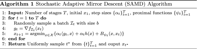
The general update rule of the Stochastic Adaptive Mirror Descent (SAMD) algorithm with proximal functions \(\psi _{t}(x)\) is defined as follows
where \(\alpha _t\) is the step size, \(g_t = \nabla f_{{\mathcal{I}}_j} (x_t)\) is the gradient from a random data batch \({\mathcal{I}}_j\), and h(x) is the regularization function on the dual space. \(B_{\psi _t}(x, x_t)\) is the Bregman divergence with respect to the proximal function \(\psi _t(x)\), defined as
Different proximal functions \(\psi _t(x)\) would generate different Bregman divergences and thus different algorithms. For example, the update rule for ProxSGD is
In this case, \(B_{\psi _t}(x, y) = \frac{1}{2}\Vert x-y\Vert _2^2\) and it is generated by the (fixed) proximal function \(\psi _t(x) = \frac{1}{2}\Vert x\Vert _2^2\). In this work, we consider the general case where the proximal functions are not pre-determined and can change over time so that our analysis can not only be applied to ProxSGD but also other adaptive algorithms. However, we need to require that the proximal functions are all m-strongly convex on the domain \({\mathcal{X}}\) for some real constant \(m > 0\).
Assumption 1
The proximal functions \(\{\psi _{t}(x)\}_{t=1}^T\) are all m-strongly convex with respect to \(\Vert \cdot \Vert _2\) on the space \({\mathcal{X}}\), i.e., for any \(x, y \in {\mathcal{X}}\)
A very important property of Bregman divergence is that \(\psi _t(x)\) is m-strongly convex with respect to the \(L_2\) norm if and only if \(B_{\psi _t}(x, y) \ge \frac{m}{2}\Vert y-x\Vert _2^2\). The constant m can be viewed as a lower bound of the strong convexity of all the proximal functions \(\{\psi _{t}(x)\}_{t=1}^T\), where T is the total number of iterations. Therefore, Assumption 1 is actually a mild assumption. Here we provide a few examples of different proximal functions that satisfy Assumption 1, and the corresponding values of m to show the cases where our general theory can be applied.
Example 1
\(\psi _{t}(x) = \phi _{t}(x) + \frac{c}{2}\Vert x\Vert _2^2\), where \(c > 0\) is a real constant and each \(\phi _{t}(x)\) is an arbitrary convex differentiable function, then \(m = c\). It can be observed that this example reduces to the ProxSGD algorithm when \(\phi _t(x) = 0\) and \(c = 1\).
Example 2
\(\psi _{t}(x) = \frac{c_t}{2}\Vert x\Vert _2^2\), where \(c_t\) is a function of t that satisfies \(c_t \ge c, \forall t \in [T]\) for some constant \(c > 0\), then \(m = c\). This case is equivalent to using time-varying step sizes in ProxSGD even when \(\alpha _t\) is fixed, because \(B_{\psi _t}(x, y) = \frac{c_t}{2}\Vert x-y\Vert _2^2\) and we can divide all terms in Eq. (2) by the time-varying \(c_t\) simultaneously. In other words, we only require the actual step sizes (\(\alpha _t /c_t\)) to be upper bounded to satisfy Assumption 1, which is natural since an unbounded step size is never favorable during the optimization process.
Example 3
\(\psi _{t}(x) = \frac{1}{2}\Vert x\Vert _p^2\), where \(1<p\le 2\), then \(m = (p-1)\) because of the following sequence of inequalities
These are standard results in convex analysis and the proof of them can be found in, e.g., Asi and Duchi (2019). As we have mentioned, such a case is especially useful when the domain \({\mathcal{X}}\) is the \(\ell _p\)-ball.
Example 4
\(\psi _{t}(x) = \frac{1}{2}\langle x, H_{t} x \rangle\), where \(H_t \in {\mathbb{R}}^{d\times d}\) and \(H_{t} \succeq c I, \forall t \in [T]\) for a constant \(c>0\), then \(m = c\). This case covers all the self-adaptive algorithms with a lower bound on the positive definiteness of the matrix \(H_t\). Such a lower bound can be guaranteed by simply adding cI to \(H_t\) when it is a non-negative diagonal matrix or by using some assumptions. More details will be discussed in Sect. 4.
Example 5
\(\psi _{t}(x) = \sum _{i=1}^d x_i \log x_i\). This case is useful when the domain is the simplex \({\mathcal{X}} = \{x \in {\mathbb{R}}^d \mid x \succeq 0, 1^Tx = 1\}\). Bregman divergence \(B_{\psi _t}(x,y)\) becomes the well-known KL divergence between x and y, and \(m = 1\).
The convergence of different algorithms in the nonconvex smooth optimization problem (i.e., when \(h(x) = 0\)) is usually represented by the stationarity of the gradient \(\nabla F(x)\), i.e., given a point \({\hat{x}}\) chosen by a stochastic algorithm, we have \({\mathbb{E}}[\Vert \nabla F({\hat{x}}) \Vert ^2] \le \epsilon\)Footnote 1. However, because of the existence of h(x) in nonsmooth nonconvex problems, we need a special definition of the generalized gradient for adaptive mirror descent algorithms and the corresponding convergence criterion in order to analyze their convergence, as in Reddi et al. (2016b) and Li and Li (2018).
Definition 1
Given a point \(x_t \in {\mathcal{X}}\), the generalized gradient \({g}_{X,t}\) is defined as \({g}_{X,t} = \frac{1}{\alpha _t}(x_t - x_{t+1}^+)\), where \(x^{+}_{t+1}\) is defined as
We define the convergence criterion to be the stationarity of the generalized gradient \({\mathbb{E}}[\Vert {g}_{X, t}\Vert ^2] \le \epsilon\). In the definition of \(x^+_{t+1}\), we replace the stochastic gradient \(g_t\) in Eq. (2) by the accurate, full-batch gradient \(\nabla f(x_t)\). In other words, \(x_{t+1}^+\) is the next-step parameter if we use the full batch gradient \(\nabla f(x_t)\) for mirror descent at time t, and \(g_{X,t}\) is the difference between \(x_t\) and \(x_{t+1}^+\) scaled by the step size. Therefore, the generalized gradient is small when \(x_{t+1}^+\) and \(x_t\) are close enough and thus the algorithm converges. We emphasize that Definition 1 and the convergence criterion are commonly observed in the mirror descent algorithm literature such as Ghadimi et al. (2016); Li and Li (2018). We provide a few examples of \(g_{X,t}\) for further clarifications. If \(\psi _t(x) = \frac{1}{2}\Vert x\Vert ^2_2\), then the definition is equivalent to the gradient mapping in Li and Li (2018). If we further assume h(x) is a constant, then Definition 1 reduces to the original full batch gradient \(\nabla f(x)\). When h(x) is a constant and \(\psi _t(x) = \frac{1}{2}\langle x, H_t x\rangle\), the generalized gradient is equivalent to \(H_t^{-1} \nabla f(x)\), which is the update of self-adaptive algorithms.
Now, for the functions \(\{f_i\}_{i=1}^n\), we assume that they have L-Lipschitz continuous gradients, which is a standard assumption in the nonconvex optimization literature (Ghadimi et al., 2016; Reddi et al., 2016b; Li & Li, 2018).
Assumption 2
Each function \(f_i(x)\) has an L-Lipschitz continuous gradient, i.e., there exists a constant \(L > 0\) such that for any \(x, y \in {\mathcal{X}}\),
As in Li and Li (2018), we use the stochastic first-order oracle (SFO) complexity to compare the convergence rates of different algorithms.
Assumption 3
When given a parameter x, SFO returns one stochastic gradient \(\nabla f_j (x)\) that is unbiased with bounded variance \(\sigma ^2\), i.e., for any \(x \in {\mathcal{X}}\)
In other words, the SFO complexity measures the number of gradient computations in the optimization process and thus how fast the algorithm converges. We summarize the SFO complexity of a few mirror descent algorithms in the nonconvex nonsmooth optimization problem in Table 1.
3.3 Assumptions and definitions for P–L condition
Next, we present the additional assumptions and definitions needed for the convergence analysis under the generalized Polyak–Lojasiewicz (P–L) condition (Polyak, 1963). The original P–L condition (in smooth problems, i.e., \(h(x) = 0\)), also known as the gradient dominant condition, is defined as
which is weaker than restricted strong convexity and it has been studied in many nonconvex convergence analyses such as Reddi et al. (2016); Zhou et al. (2018b); Lei et al. (2017). However, because of the existence of h(x) in nonsmooth problems, the original P–L condition is no longer useful. Instead, we utilize the definition of the generalized gradient \(g_{X,t}\) to define the generalized P–L condition as follows.
Definition 2
The loss function F(x) satisfies the generalized P–L condition if
where \(g_{X,t}\) is the generalized gradient defined in Definition 1.
Li and Li (2018) used a similar definition of the general P–L condition when \(\psi _t(x) = \frac{1}{2}\Vert x\Vert _2^2\), and ours is a natural extension since we consider general proximal functions in Eq. (2). The above definition reduces to the P–L condition by Li and Li (2018) when \(\psi _t(x) = \frac{1}{2}\Vert x\Vert _2^2\). If we further assume that h(x) is a constant, then Definition 2 is the same as the original P–L condition. For simplicity, we further assume that the constant \(\mu\) satisfies \(L/(m^2\mu ) \ge \sqrt{n}\), similar to what Li and Li (2018); Reddi et al. (2016b) assumed in their papers. The condition is similar to the “high condition number regime” for strongly convex optimization problems. It is noticeable that given the general P–L condition, the original convergence criterion \(({\mathbb{E}}[\Vert g_{X,t}\Vert ^2] \le \epsilon )\) is equivalent to
which means that the algorithm converges to the global minimum. The SFO complexity of a few mirror descent algorithms in the generalized P–L conditioned problem is also provided in Table 1.
4 Algorithm and convergence
In this section, we present our main theoretical results. In Sect. 4.1, we provide the convergence rate of the general stochastic adaptive mirror descent algorithm as a competitive baseline, which matches the best existing rates of non-adaptive mirror descent algorithms. In Sects. 4.2, 4.3, and 4.4, we present our generalized variance reduced mirror descent algorithm framework SVRAMD and provide its convergence analysis to show that variance reduction can accelerate the convergence of most adaptive mirror descent algorithms in both the nonconvex nonsmooth problem and the generalized P–L conditioned problem.
4.1 The adaptive mirror descent algorithm and its convergence
We first provide the the SFO complexities of the general Stochastic Adaptive Mirror Descent (SAMD) algorithm (Algorithm 1) in the nonconvex nonsmooth problem and the generalized P–L conditioned problem as the baseline, which are to the best of our knowledge, very important results but has not been established in literature. We prove that in both problems, the convergence rates of Algorithm 1 are similar to those of the non-adaptive mirror descent algorithm (Ghadimi et al., 2016), (Karimi et al., 2016). The proof of these important baseline SFO complexities are provided in Appendix A for the readers’ reference.
Theorem 1
Suppose that Assumption 1, 2, 3are satisfied. Set the learning rate and the mini-batch size in Algorithm 1 to be \(\alpha _t = m/L, b = n \wedge ({12\sigma ^2}/(m^2\epsilon ))\), then the output of Algorithm 1 converges with SFO complexity
Remarks. The above complexity can be treated as \(O(n\epsilon ^{-1} \wedge \epsilon ^{-2})\) and it is the same as the complexity of non-adaptive mirror descent algorithms by Ghadimi et al. (2016). Algorithm 1 needs a relatively large mini-batch size (\(b = O(\epsilon ^{-1})\)) to obtain a convergence rate close to that of ProxGD (\(O(n\epsilon ^{-1})\)) and ProxSGD (\(O(\epsilon ^{-2})\)) (Reddi et al., 2016). However, it is still only asymptotically as fast as the faster one between ProxGD and ProxSGD, depending on whether \(\epsilon ^{-1}\) is larger than the sample size n. Next we provide the convergence rate of Algorithm 1 in the generalized P–L conditioned problem.
Theorem 2
Suppose that Assumption 1, 2, 3are satisfied. Further assume that the loss function F(x) satisfies the generalized P–L condition (Definition 2). Set the learning rate and the mini-batch sizes in Algorithm 1 to be \(\alpha _t = m/L, b_t = n~ \wedge ~({2(1+m^2)\sigma ^2}/(\epsilon m^2\mu ))\), then the output of Algorithm 1 converges with SFO complexity
Remarks
The above result is of order \(O \left( \left( n \wedge \frac{1}{\epsilon }\right) \log \frac{1}{\epsilon } \right)\). Similar to Theorem 1, the proved SFO complexity matches the smaller complexity of ProxSGD and ProxGD in the generalized P–L conditioned problem (Karimi et al., 2016). We emphasize that since the general Algorithm 1 covers ProxSGD (\(b=1\)) and ProxGD (\(b=n\)) with \(\psi _t(x) = \frac{1}{2}\Vert x\Vert _2^2\) as special cases, we believe that our convergence rates in Theorems 1 and 2 are the best rates achievable and serve as strong baselines.
4.2 The general variance reduced algorithm-SVRAMD
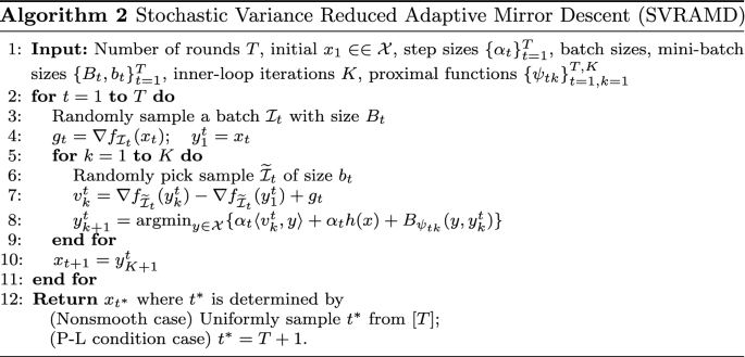
We now present the proposed Stochastic Variance Reduced Adaptive Mirror Descent (SVRAMD) algorithm, which is a simple and generalized variance reduction framework for different mirror descent algorithm designed for different parameter domains \({\mathcal{X}}\). We provide the pseudo-code in Algorithm 2. The input parameters \(B_t\) and \(b_t\) are called the batch sizes and the mini-batch sizes. The algorithm consists of two loops: the outer loop has T iterations while the inner loop has K iterations. At each iteration of the outer loop (line 4), we estimate a large batch gradient \(g_t = \nabla f_{{\mathcal{I}}_t}({x}_{t})\) with batch size \(B_t\) at the reference point \(x_t\), both of which will be stored during the inner loop. At each iteration of the inner loop (line 7), the large batch gradient is used to reduce the variance of the small batch gradient \(\nabla f_{\widetilde{{\mathcal{I}}}_t}(y_{k}^t)\) so that the convergence becomes more stable. Note that in line 8, the proximal function is an undetermined \(\psi _{tk}(x)\) which can change over time, therefore Algorithm 2 covers ProxSVRG+ and a lot more algorithms with different proximal functions. For example, if \(\psi _{tk}(x) = \frac{1}{2}\Vert x\Vert _2^2\), then \(B_{tk}(y, y_k^t) = \frac{1}{2}\Vert y - y_k^t\Vert _2^2\) and SVRAMD reduces to ProxSVRG+ (Li & Li, 2018). If \(\psi _{tk}(x) = \frac{1}{2} \langle x, H_{tk}x \rangle\), where \(H_{tk} \succeq mI\), then SVRAMD reduces to variance reduced self-adaptive algorithms for different matrices \(H_{tk}\), e.g., VR-AdaGrad in Sect. 4.5.
4.3 Nonconvex nonsmooth convergence
Now given the general form of Algorithm 2, we provide its SFO complexity in the nonconvex nonsmooth problem in the following theorem.
Theorem 3
Suppose that Assumption 1, 2, 3are satisfied. Set the learning rate, the batch sizes, the mini-batch sizes, and the number of inner-loop iterations in Algorithm 2 to be \(\alpha _t = m/L, ~ B_t = n \wedge ({20\sigma ^2}/m^2\epsilon ), ~b_t = b, ~K = \left\lfloor {\sqrt{b/20}}\right\rfloor \vee 1\), then the output of Algorithm 2 converges with SFO complexity
Remarks
The proof is relegated to Appendix B. Theorem 3 essentially claims that with Assumptions 1, 2, 3, we can guarantee the SFO complexity of Algorithm 2 is \(O \left( \frac{n}{\epsilon \sqrt{b}} \wedge \frac{\sigma ^2}{\epsilon ^2\sqrt{b}} + \frac{b}{\epsilon } \right)\), with an undetermined mini-batch size b to be tuned later.
Although \(\alpha _t\) is fixed in the theorem, \(\psi _{tk}\) can change over time and hence results in the adaptivity in the algorithm. For example, our theory indicates that using time-varying dynamic step sizes is allowed during the optimization process (Example 2 in Sect. 3). When we take the proximal function to be \(\psi _{tk}(x) = \frac{c_{tk}}{2}\Vert x\Vert _2^2, c_{tk} \ge m\), Algorithm 2 uses time-varying dynamic effective step size \(\alpha _t/c_{tk}\) (i.e., the same as \(\eta _t\) in Li and Li (2018)). As long as the effective step sizes \(\alpha _t/c_{tk}\) are upper bounded by the constant \((m/L)/m = 1/L\), Algorithm 2 still converges with the same complexity. Such a constraint is easy to satisfy for many step size schedules such as (linearly) decreasing step sizes, cyclic step sizes and warm up. Besides, \(\psi _{tk}\) can be even more complicated, such as Examples 1 and 4 we have mentioned in Sect. 3, which will be discussed later. Another interesting result observed in our theorem is that when m is small, we require a relatively larger batch size \(B_t\) to guarantee the fast convergence rate. We will later show that this intuition is actually supported by our experiments in Sect. 5.
While SCSG (Lei et al., 2017) and ProxSVRG (Reddi et al., 2016b) achieve their best convergence rate at either a too small or a too large mini-batch size, i.e., \(b =1\) or \(b=n^{2/3}\), our algorithm achieves its best performance using a moderate mini-batch size \(\epsilon ^{- 2/3}\). We provide the following corollary.
Corollary 1
Under all the assumptions and parameter settings in Theorem 3, further take \(b = \epsilon ^{- 2/3} \le n\), then the output of Algorithm 2 converges with SFO complexity
Remarks
The above SFO complexity is provably better than the SFO complexity of the SAMD algorithm in Theorem 1. Note that the number of samples is usually very large in modern datasets, such as \(n = 10^6\), thus \(b = \epsilon ^{- 2/3}\le n\) can be easily satisfied with a constant mini-batch size and a small enough \(\epsilon\), such as \(b=10^2, \epsilon = 10^{-3}\). If the above best complexity cannot be achieved, meaning that either n or \(\epsilon\) is too small, some sub-optimal solutions are still available for fast convergence. For example, setting \(b = n^{2/3}\) would generate \(O(n^{2/3}\epsilon ^{-1})\) SFO complexity, which is also smaller than the SFO complexity of Algorithm 1. Therefore, we conclude that if the parameters are carefully chosen, variance reduction can reduce the SFO complexity and accelerate the convergence of any adaptive mirror descent algorithm that satisfies Assumption 1 in the nonsmooth nonconvex problem. We summarize the SFO complexity generated by a few different choices of b in the nonconvex nonsmooth problem in Table 2.
As can be observed in Table 1 and 2, the SFO complexity of SVRAMD is the same as the best SFO complexity of ProxSVRG+ and SCSG in the nonsmooth problem. Although it is slightly worse than the-state-of-the-art SFO complexity of some optimization algorithms in \({\mathbb{R}}^d\) (e.g., the complexity of PAGE (Li et al., 2021)), we emphaisze that our paper is the first step towards proving that the simple variance reduction technique can accelerate most adaptive mirror descent algorithms. Whether it is possible to achieve the state-of-the-art complexity for different mirror descent algorithms on different domains \({\mathcal{X}}\) still remain interesting open questions. Moreover, we will show that our algorithm achieves the state-of-the-art complexity in the generalized P–L conditioned problem in the next subsection.
4.4 Convergence under the generalized P–L condition
Now we provide the convergence analysis of Algorithm 2 under the generalized P–L condition (Definition 2). Note that the only difference in Algorithm 2 for such problems is the final output, where we directly use the last \(x_{T+1}\) rather than randomly sample from the historical \(x_t\)s. Therefore, we preserve the simplicity of our algorithm in both the nonconvex nonsmooth problem and the generalized P–L conditioned problem. Now we present the SFO complexity of SVRAMD under the generalized P–L condition and show its linear convergence rate.
Theorem 4
Suppose that Assumption 1, 2, 3are satisfied. Further assume that F(x) satisfies the generalized P–L condition (Definition 2). Set the learning rate, the batch sizes, the mini-batch sizes, and the number of inner loop iterations in Algorithm 2 to be \(\alpha _t = m/L, ~B_t = n \wedge ({10\sigma ^2}/({\epsilon m^2\mu })), ~b_t = b, ~K = \lfloor {\sqrt{b/32}} \rfloor \vee 1\), then the output of Algorithm 2 converges with SFO complexity
Remarks
The proof is provided in Appendix C. The above SFO complexity is of size \({\widetilde{O}}((n \wedge ( \epsilon )^{-1})b^{-1/2} + b)\) if we hide the logarithm terms. Compared with the SFO complexity of the SAMD algorithm, our complexity can be arguably smaller when we choose an appropriate mini-batch size b, which further proves our conclusion that variance reduction can be applied to most adaptive mirror descent algorithms to accelerate their convergence. We provide the following corollary for the best choice of b to show its effectiveness.
Corollary 2
Under all the assumptions and parameter settings in Theorem 4, further take \(b = (\mu \epsilon )^{- 2/3} \le n\). Then the output of Algorithm 2 converges with SFO complexity
Remarks
The above complexity is provably better than the SFO complexity of SAMD in Theorem 2. Moreover, our algorithm is so simple that it does need to perform any restart (as in ProxSVRG and ProxSAGA (Reddi et al., 2016b)) or use the stochastically controlled iterations or probability estimators tricks (as in SCSG and PAGE (Lei & Jordan, 2020; Li et al., 2021)). Therefore, Algorithm 2 automatically switches to fast convergence in regions satisfying the generalized P–L condition. We also provide the SFO complexity of some other choices of b in Table 2 for a clearer comparison. Similarly, if \(b = (\mu \epsilon )^{- 2/3}\) is impractical, using \(b = n^{2/3}\) also generates faster convergence than SAMD.
As can be observed in Tables 1 and 2, because in Corollary 2 we take \(b = (\mu \epsilon )^{-2/3} \le n\) and thus our \(O \left( \frac{1}{\epsilon ^{2/3}}\log \frac{1}{\epsilon } \right)\) complexity is better than the \(O \left( n \log \frac{1}{\epsilon } \right)\) complexity of PAGE (Li et al., 2021). Similar conclusions can be drawn for the case \(b = n^{2/3}\). The SFO complexity in Corollary 2 matches the complexity of ProxSVRG+, which is the state-of-the-art complexity in the generalized P–L conditioned problem. Therefore, we conclude that SVRAMD achieves comparable performances in both the nonsmooth problem and the P–L conditioned problem, and it accelerates SAMD.
4.5 Special case: self-adaptive algorithms
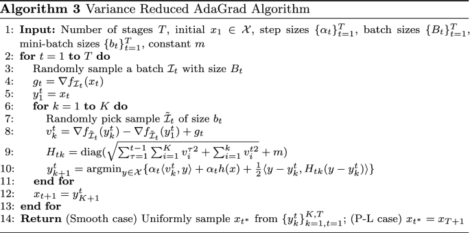
As we have mentioned in Sect. 3, self-adaptive algorithms such as AdaGrad are special cases of the general Algorithm 1 and thus we can use Algorithm 2 to accelerate them. The proximal functions of most adaptive algorithms have the form of \(\psi _t(x) = \frac{1}{2}\langle x, H_t x \rangle\), where \(H_t \in {\mathbb{R}}^{d\times d}\) is often designed to be a diagonal matrix.
Assumption 1 is satisfied if we consistently add a constant matrix mI to \(H_t\), with I being the identity matrix. We remark that such an operation is commonly used in self-adaptive algorithms to avoid division by zero or improper inverse operations (Duchi et al., 2010; Kingma & Ba, 2015), and thus variance reduction can be applied. Assumption 1 can also be satisfied for many special designs of \(H_t\) with some mild assumptions. For example, if \(H_{t,ii} = \sqrt{g_{1,i}^2 + g_{2,i}^2 + \cdots g_{t,i}^2}, \forall i \in [d]\) (the original AdaGrad algorithm), then \(H_{t} \succeq m I\) if there exists one \(\tau _i \in [t]\) on each dimension i such that \(g_{\tau _i, i} \ge m\), meaning that there is at least one derivative larger than m on each dimension in the whole optimization process. If such a mild condition holds, then the conclusions in Theorem 3, 4 and Corollary 1, 2 still hold.
However, notice that the strong convexity lower bounds of these algorithms are relatively smaller (the constant m in the added matrix mI is often set as 1e-2 or even smaller in real experiments), Theorem 3 implies that the batch size \(B_t\) needs to be sufficiently large for these algorithm to converge fast. If variance reduction can work with such algorithms with small m, then we should expect good performances with the other algorithms that have large m’s. We provide the implementation for Variance Reduced AdaGrad (VR-AdaGrad) in Algorithm 3 and Variance Reduced RMSProp (VR-RMSProp) is similar.
One interesting question here is whether VR-AdaGrad and VR-RMSProp can converge even faster in nonconvex nonsmooth problems or generalied P–L conditioned problems, since AdaGrad and RMSProp are known to converge faster than SGD in convex problems. Our conjecture is that they cannot do so, at least not in the nonconvex case because their rapid convergence relies on not only the convexity of the problem, but also the sparsity of the gradients (Duchi et al., 2011). If neither of these two assumptions is assumed, we believe it would be difficult to prove any superiority of AdaGrad/RMSProp.
5 Experiments
In this section, experimental results are provided to validate our theoretical claims.
5.1 Synthetic data experiments
We first provide some preliminary experimental results on synthetic data to prove the correctness of our theory. We choose the task of regularized linear regression \(F(x) = \frac{1}{n}\Vert Ax-y\Vert _2^2 + c \Vert x\Vert _2^2\) with \(A \in {\mathbb{R}}^{n \times d}\) and \(x \in {\mathcal{X}} \subseteq {\mathbb{R}}^d\). We set the domain to be \({\mathcal{X}} = \{ x \in {\mathbb{R}}^d \mid \Vert x\Vert _{\infty } \le 1\}\). Each entry of the target \(x^*\) is generated from \({\mathcal{X}}\) uniform randomly. The rows of A are generated uniform randomly from the standard basis of \({\mathbb{R}}^{d}\) and the observation \(y \in {\mathbb{R}}^n\) is generated by \(y = Ax^* + v\), where \(v \sim {\mathcal{N}}(0, I_n)\). We examine our theoretical claims with different choices of the proximal functions, i.e., the case \(\frac{1}{2}\Vert x\Vert _2^2\), which we call SAGD and SVRAGD for Algorithm 1 and 2 respectively in Fig. 1 to avoid confusions, and the adaptive case \(\frac{1}{2}\langle x, H_t x \rangle\) where \(H_t\) is taken to be the diagonal matrices in AdaGrad, RMSProp, VR-AdaGrad, and VR-RMSProp (as discussed in Sect. 4.5). The hyper-parameters of aforementioned algorithms such as the learning rate, the batch sizes are chosen to be exactly the same as in Theorem 1 and 3. As shown in Fig. 1, variance-reduced algorithms converge much faster than the baseline algorithms in both the two cases \(d=10\) and \(d=50\), showing that our proposed method of variance reduction is effective. More details of our synthetic experiments can be found in Appendix D.2.

Performance of SAGD, SVRAGD, AdaGrad, RMSProp, VR-AdaGrad, and RMSProp on synthetic linear regression data. a training loss when \(d=10\) b training loss when \(d=50\)
5.2 Deep learning experiments
We then present several experiments on training both shallow and deep neural networks on image datasets to further show the effectiveness of variance reduction in the SVRAMD algorithm, which are known to have highly nonconvex loss landscapes. Specifically, we train a two-layer fully connected network on the MNIST dataset, the LeNet (LeCun et al., 1998) on the CIFAR-10 dataset, and the ResNet-20 model on the CIFAR-100 dataset (He et al., 2016).
In general, we have followed the settings by Zhou et al. (2018b) on SNVRG for all our experiments. Except for normalization, we do not perform any additional data transformation or augmentation techniques such as rotation, flipping, and cropping on the images. Our code is based on publicly released PyTorch code.Footnote 2 All experiments here are conducted on one Nvidia V100 GPU. We have thoroughly tuned the hyper-parameters for all the algorithms. One important remark here is that for the batch sizes and mini batch sizes \(B_t\) and \(b_t\), we follow Zhou et al. (2018b) to use a slightly different but equivalent notation of batch size ratio \(r = B_t/b_t\). Increasing this ratio when \(b_t\) is fixed would be the same as increasing the batch size \(B_t\). More details of our deep learning experiments can be found in Appendix D.3.

Performance of SAMD and SVRAMD with different step size schedules. The solid lines are trained with the warmup schedule (warmup for 5 epochs then step decay) and the dashed lines are trained with the warm restart schedule. We plot the two schedules at the top-right corners of the training loss subfigures for the readers’ reference. a, b training loss and testing accuracy using fully connected network on MNIST. c, d training loss and testing accuracy using LeNet on CIFAR-10. The results were averaged over 5 runs

a, d: training loss and testing accuracy on MNIST. b, e: training loss and testing accuracy on CIFAR-10. c and f: training loss and testing accuracy on CIFAR-100. The results are averaged over 5 runs

a, d: training loss with different r on MNIST. b, e training loss with different r on CIFAR10 . c, f training loss with different ratio r on CIFAR100
We first validate our claims in Sect. 4 by showing that variance reduction can work well with different step size schedules. We choose two special schedules that are both complicated enough and popular nowadays, warm up and warm restart. The proximal functions are set to be \(\frac{1}{2\alpha _t}\Vert x\Vert _2^2\), where \(\alpha _t\) is the step size. For warm up, we increase the step size from zero to the best step size of SAMD/SVRAMD linearly for the initial 5 epochs and then multiply the step size by 0.1 at the 50-th and the 75-th epoch. For warm restart, we decrease from the best step size to zero with cosine annealing in 50 epochs and then restart the decay. The training loss, the testing accuracy and the step size schedules on MNIST and CIFAR-10 are plotted in Fig. 2. As can be seen in the figures, converges faster than SAMD with both of the two special step size schedules, proving our claim that as long as the step sizes are bounded, variance reduction can still improve the convergence rate of SAMD with dynamic step sizes.
We then choose VR-AdaGrad and VR-RMSProp as the other two special examples of our general algorithm because they have relatively smaller lower bound of the strong convexity and their proximal functions are even more complicated. We use the constant step size schedule for these algorithms as they are self-adaptive. The training loss and the testing Top-1 accuracy of VR-AdaGrad, VR-RMSProp, and their original algorithms on all the three datasets are plotted in Fig. 3. As can be observed, the variance reduced algorithms converge faster than their original algorithms and their best testing Top-1 accuracy is also comparable or even higher, proving the effectiveness of variance reduction. We emphasize that the experiments are not designed to pursue the state-of-the-art performances, but to show that variance reduction can work well with any adaptive proximal functions and contribute to faster training, even if the proximal functions have very small strong convexity lower bound.
Finally, we also show that algorithms with weaker convexity need a larger batch size \(B_t\) to converge fast, which corresponds to our claims in Sects. 4.3 and 4.4. We fix the mini batch sizes \(b_t\) in VR-AdaGrad and VR-RMSProp to be the same as in the previous experiments and gradually increase the batch size ratio r. The baseline ratios of ProxSVRG+, which has a large strong convexity lower bound, are provided in Appendix D for the readers’ reference and the training performances of VR-AdaGrad and VR-RMSProp with different r are shown in Fig. 4. Note that ProxSVRG+ only needs a small ratio (\(r=4\) or \(r=8\)) to be faster than SGD (Li & Li, 2018), but for VR-RMSProp, even when \(r = 16\), the algorithms still do not converge faster than RMSProp, proving that algorithms with weaker convexity need larger batch sizes \(B_t\) to show the effectiveness of variance reduction.
6 Conclusions and future works
In this work, we provide the first algorithmic framework for accelerating adaptive mirror descent algorithms in different parameter domains using variance reduction. Theoretically, we prove that the proposed SVRAMD algorithm improves the convergence rates of adaptive mirror descent algorithms under a very mild assumption, both in the general nonsmooth nonconvex problems and the generalized P–L conditioned problems. Our theoretical results even match the state-of-the art results in the generalized P–L conditioned problems. Based on the generality of our algorithmic framework and the analysis, our theory can be applied to many different problems, such as (1). proving the soundness of using time-varying step sizes in the training process of SVRAMD, and (2). the effectiveness of applying variance reduction to adaptive algorithms such as AdaGrad and RMSProp. A potential future work direction is whether our Assumption 1 can still be replaced by weaker conditions, such as the CHEF conditions Lei and Jordan (2020) have mentioned in the convex case. Another interesting direction is whether the SFO complexity in the nonconvex nonsmooth problem can be further improved with the help of additional algorithmic components, for example, the nested variance reduction technique by Zhou et al. (2018b), momentum accelerations by Allen-Zhu (2017), or the probabilistic estimators by Li et al. (2021).
Data availability
The data is publicly available
Code availability
The source code is publicly available.
Notes
Some works such as Zhou et al. (2018b) use \({\mathbb{E}}[\Vert \nabla F({\hat{x}}) \Vert ^2] \le \epsilon ^2\) instead of our choice. To compare our results with theirs, simply replace all the \(\epsilon\) in our results by \(\epsilon ^2\).
References
Allen-Zhu, Z. (2017). Natasha: Faster non-convex stochastic optimization via strongly non-convex parameter. In Proceedings of international conference on machine learning.
Allen-Zhu, Z. (2018). Natasha 2: Faster non-convex optimization than SGD. Advances in Neural Information Processing Systems.
Asi, H., & Duchi, J. C. (2019). Modeling simple structures and geometry for better stochastic optimization algorithms. In Proceedings of international conference on artificial intelligence and statistics.
Chen, X., Liu, S., Sun, R., & Hong, M. (2019). On the convergence of a class of adam-type algorithm for non-convex optimization.
Defazio, A., Bach, F., & Lacoste-Julien, S. (2014). Saga: A fast incremental gradient method with support for non-strongly convex composite objectives. Advances in Neural Information Processing Systems
Dubois-Taine, B., Vaswani, S., Babanezhad, R., Schmidt, M., & Lacoste-Julien, S. (2021). SVRG meets AdaGrad: Painless variance reduction. arXiv: 2102.09645
Duchi, J., Shalev-Shwartz, S., Singer, Y., & Tewari, A. (2010). Composite objective mirror descent. In Proceedings of the twenty third annual conference on computational learning theory.
Duchi, J., Hazan, E., & Singer, Y. (2011). Adaptive subgradient methods for online learning and stochastic optimization. Journal of Machine Learning Research12(7).
Fang, C., Li, C. J., Lin, Z., & Zhang, T. (2018). SPIDER: Near-optimal non-convex optimization via stochastic path-integrated differential estimator. Advances in Neural Information Processing Systems.
Ge, R., Li, Z., Wang, W., & Wang, X. (2019). Stabilized SVRG: Simple variance reduction for nonconvex optimization. In Conference on learning theory.
Gentile, C. (2003). The robustness of the \(p\)-norm algorithms. Machine Learning, 53, 265–299.
Ghadimi, S., Lan, G., & Zhang, H. (2016). Mini-batch stochastic approximation methods for nonconvex stochastic composite optimization. arXiv preprint arXiv:1308.6594
Goyal, P., Dollár, P., Girshick, R., Noordhuis, P., Wesolowski, L., Kyrola, A., Tulloch, A., Jia, Y., & He, K. (2017). Accurate, large minibatch SGD: Training ImageNet in 1 hour. 1706.02677.
He, K., Zhang, X., Ren, S., & Sun, J. (2016). Deep residual learning for image recognition. In IEEE conference on computer vision and pattern recognition.
Huang, H., Wang, C., & Dong, B. (2019). Nostalgic adam: Weighting more of the past gradients when designing the adaptive learning rate. arXiv preprint arXiv: 1805.07557
Johnson, R., & Zhang, T. (2013). Accelerating stochastic gradient descent using predictive variance reduction. Advances in Neural Information Processing Systems.
Karimi, H., Nutini, J., & Schmidt, M. (2016). Linear convergence of gradient and proximal-gradient methods under the Polyak-łojasiewicz condition.
Kingma, D. P., & Ba, J. L. (2015). Adam: A method for stochastic optimization. In Proceedings of the 3rd international conference on learning representations (ICLR).
Krizhevsky, A., Nair, V., & Hinton, G. (2009). Cifar-10 (Canadian Institute for Advanced Research). 1.
LeCun, Y., Bottou, L., Bengio, Y., & Haffner, P. (1998). Gradient-based learning applied to document recognition. Proceedings of the IEEE, 86(11), 2278–2324.
Lei, L., & Jordan, M. I. (2020). On the adaptivity of stochastic gradient-based optimization. SIAM Journal on Optimization, 30(2), 1473–1500.
Lei, L., Ju, C., Chen, J., & Jordan, M. I. (2017). Non-convex finite-sum optimization via SCSG methods. Advances in Neural Information Processing Systems, 30, 2348–2358.
Li, W., Zhang, Z., Wang, X., & Luo, P. (2020). Adax: Adaptive gradient descent with exponential long term memory. arXiv preprint arXiv:2004.09740
Li, Z., & Li, J. (2018). A simple proximal stochastic gradient method for nonsmooth nonconvex optimization. Advances in Neural Information Processing Systems, 31, 5564–5574.
Li, Z., Bao, H., Zhang, X., & Richtárik, P. (2021). PAGE: A simple and optimal probabilistic gradient estimator for nonconvex optimization. In International conference on machine learning.
Liu, L., Jiang, H., He, P., Chen, W., Liu, X., Gao, J., & Han, J. (2019). On the variance of the adaptive learning rate and beyond. arXiv preprint arXiv:1908.03265
Liu, M., Zhang, W., Orabona, F., & Yang, T. (2020). Adam\(^+\): A stochastic method with adaptive variance reduction. arXiv: 2011.11985
Loshchilov, I., & Hutter, F. (2016). SGDR: Stochastic gradient descent with warm restarts. In International conference on learning representations.
Luo, L., Xiong, Y., Liu, Y., & Sun, X. (2019). Adaptive gradient methods with dynamic bound of learning rate. In Proceedings of 7th international conference on learning representations.
Nair, V., & Hinton, G. (2010). Rectified linear units improve restricted Boltzmann machines. In Proceedings of 27th international conference on machine learning (ICML).
Pham, N. H., Nguyen, L. M., Phan, D. T., & Tran-Dinh, Q. (2020). ProxSARAH: An efficient algorithmic framework for stochastic composite nonconvex optimization. Journal of Machine Learning Research, 21(110), 1–48.
Pham, N. H., Nguyen, L. M., Phan, D. T., & Tran-Dinh, Q. (2021). A hybrid stochastic optimization framework for composite nonconvex optimization. Mathematical Programming A.
Polyak, B. T. (1963). Gradient methods for minimizing functionals. Zhurnal Vychislitel’noi Matematiki i Matematicheskoi Fiziki.
Reddi, S., Sra, S., Poczos, B., & Smola, A. J. (2016b). Proximal stochastic methods for nonsmooth nonconvex finite-sum optimization. Advances in Neural Information Processing Systems.
Reddi, S. J., Hefny, A., Sra, S., Poczos, B., & Smola, A. (2016). Stochastic variance reduction for nonconvex optimization. In International conference on machine learning (pp. 314–323).
Schölkopf, B., & Smola, A. J. (2002). Learning with kernels: Support vector machines, regularization, optimization, and beyond. MIT Press.
Tieleman, T., & Hinton, G. (2012). RMSProp: Divide the gradient by a running average of its recent magnitude. COURSERA: Neural Networks for Machine Learning, 4(2), 26–31.
Wang, Z., Ji, K., Zhou, Y., Liang, Y., & Tarokh, V. (2019). SpiderBoost and momentum: Faster variance reduction algorithms.
Wilson, A. C., Roelofs, R., Stern, M., Srebro, N., & Recht, B. (2017). The marginal value of adaptive gradient methods in machine learning. Advances in Neural Information Processing Systems.
Zaheer, M., Reddi, S., Sachan, D., Kale, S., & Kumar, S. (2018). Adaptive methods for nonconvex optimization. Advances in Neural Information Processing Systems.
Zhou, D., Tang, Y., Yang, Z., Cao, Y., & Gu, Q. (2018a). On the convergence of adaptive gradient methods for nonconvex optimization. 1808.05671.
Zhou, D., Xu, P., & Gu, Q. (2018b). Stochastic nested variance reduction for nonconvex optimization. Advances in Neural Information Processing Systems.
Zhuang, J., Tang, T., Ding, Y., Tatikonda, S., Dvornek, N., Papademetris, X., & Duncan, J. S. (2020). AdaBelief optimizer: Adapting stepsizes by the belief in observed gradients. Advances in Neural Information Processing Systems.
Funding
Not Applicable.
Author information
Authors and Affiliations
Contributions
WL is responsible for writing the main paper and the proofs. WL and ZW are responsible for running the experiments. YZ and GC are responsible for giving work directions and revising the manuscript.
Corresponding author
Ethics declarations
Conflict of interest
The authors have no conflicts of interest to declare that are relevant to the content of this article.
Ethics approval
This paper is approved in ethics.
Consent to participate
This paper is consented to participate.
Consent for publication
This paper is consented for publication.
Additional information
Editor: Lam M. Nguyen.
Publisher's Note
Springer Nature remains neutral with regard to jurisdictional claims in published maps and institutional affiliations.
Appendices
Appendix
A Convergence of the SAMD algorithm
Before the analysis, we introduce the following notation.
Definition 3
We define the generalized stochastic gradient at t as
where \(x_t\) and \(x_{t+1}\) are from the general mirror descent algorithm in Eq. (2).
1.1 A.1 Auxiliary Lemmas
Lemma 1
(Lemma 1 in Ghadimi et al. (2016)). Let \(g_t\) be the stochastic gradient in Algorithm 1 obtained at t and \(\tilde{g}_{X,t}\) be defined as in Definition 3, then
Proof
By the optimality of the mirror descent update rule, it implies for any \(x \in {\mathcal{X}}\) and \(\nabla h(x_{t+1}) \in \partial h(x_{t+1})\), we have
Let \(x = x_t\) in the above in equality, we get
where the second inequality is due to the strong convexity of the function \(\psi _t(x)\) and the convexity of h(x), by noting that \(x_{t} - x_{t+1} = \alpha _t \tilde{g}_{X,t}\) , the inequality follows.\(\square\)
Lemma 2
Let \({g}_{X,t}, \tilde{g}_{X,t}\) be defined as in Definition 1and Definition 3respectively, then
Proof
By the definition of \(g_{X, t}\) and \(\tilde{g}_{X,t}\),
Similar to Lemma 1, by the optimality of the mirror descent update rule, we have the following two inequalities for any \(x \in {\mathcal{X}}\)
Take \(x = x_{t+1}^+\) in the first inequality and \(x = x_{t+1}\) in the second one, we can get
Summing up the above inequalities, we can get
Therefore by the Cauchy-Schwarz inequality,
Hence the inequality in the lemma follows.\(\square\)
Lemma 3
(Lemma A.1 in Lei et al. (2017)). Let \(x_1, \cdots , x_M \in {\mathbb{R}}^d\) be an arbitrary population of M vectors with the condition that
Further let J be a uniform random subset of \(\{1, \cdots , M\}\) with size m, then
Proof of the above general lemma can be found in Lei et al. (2017).
1.2 A.2 Convergence of SAMD in the nonconvex nonsmooth problem
Proof of Theorem 1
From the L-Lipshitz gradients and Lemma 1, we know that
Therefore since \(F(x) = f(x) + h(x)\), we get
where the second last one is a direct result from Cauchy-Schwarz inequality and the last inequality is from Lemma 2. Rearrange the above inequalities and sum up from 1 to T, we get
where the last inequality is due to \(F^* \le F(x), \forall x\). Define the filtration \({\mathcal{F}}_t = \sigma (x_1, \cdots , x_t)\). Note that we suppose \(g_t\) is an unbiased estimate of \(\nabla f(x_t)\), hence \({\mathbb{E}}[\langle \nabla f(x_t) -g_t, g_{X,t} \rangle | {\mathcal{F}}_t]= 0\). Moreover, since the sampled gradients has bounded variance \(\sigma ^2\), hence by applying Lemma 3 with \(x_i = \nabla _{i \in {\mathcal{I}}_j} f_i(x_t) - \nabla f(x_t)\)
where I is the indicator function. Since the final \(x_{t^*}\) is uniformly sampled from all \(\{x_{t}\}_{t=1}^T\), therefore
Therefore when \(\alpha _t, b_t\) are constants, the average can be found as
where we define \(\varDelta _F = F(x_1) - F^*\). Take \(\alpha _t = \frac{m}{L}\), then \(\alpha _t m - \frac{L}{2}\alpha _t^2 = \frac{m^2}{2L}\) and
Also by Lemma 2, the difference between \(g_{X,t^*}\) and \(\tilde{g}_{X, t^*}\) are bounded, hence
Take \(b_t = n \wedge ({12\sigma ^2}/m^2\epsilon ), T = 1 \vee (8\varDelta _F L / m^2 \epsilon )\) as in the theorem, the expectation is
Therefore since one iteration takes \(b_t\) stochastic gradient computations, the total number of stochastic gradient computations is
\(\square\)
1.3 A.3 Convergence of SAMD under the P–L condition
Proof of Theorem 2
By the proof in A.2, we have
Take expectation on both sides, we know that
Since
Hence the inequality becomes
Take \(\alpha _t = m/L\) and minus \(F(x)^*\) on both sides, we get
Let \(\gamma = 1 - \frac{\mu m^2}{2L}\), since \(m^2\mu / L \le \frac{1}{\sqrt{n}}\), \(\gamma \in (0, 1)\), divide by \(\gamma ^{t+1}\) on both sides, we get
Take summation with respect to the loop parameter t from \(t=1\) to \(t = T\), assume that \(b_t\) is a constant, the inequality becomes
Therefore when taking \(T = 1 \vee (\log \frac{2\varDelta _F}{\epsilon })/({\log \frac{1}{\gamma }}) = O(\log \frac{2\varDelta _F}{\epsilon }/\mu )\), \(b_t = n \wedge \frac{2(1+m^2)\sigma ^2}{\epsilon m^2\mu }\). Then the total number of stochastic gradient computations is
\(\square\)
B Convergence of SVRAMD in the nonconvex nonsmooth problem
Recall the Algorithm 2 in the algorithm section, similarly define
Definition 4
We define the variance reduced stochastic generalized gradient as
Definition 5
We define the variance reduced (non-stochastic) generalized gradient as
1.1 B.1 Auxiliary Lemmas
Lemma 4
Let \(v^t_k\) be defined as in Algorithm 2 and \(\tilde{g}_{Y,k}^t\) be defined as in Definition 4, then we have
Proof
The proof of this inequality is similar to that of Lemma 1. By the optimality of the mirror descent update rule, it implies for any \(y \in {\mathcal{X}}, \nabla h(y_{k+1}^t) \in \partial h(y_{k+1}^t)\),
Let \(x = y_{k}^t\) in the above in equality, we get
where the second inequality is due to the m-strong convexity of the function \(\psi _{tk}(x)\) and the convexity of h. Note from the definition that \(y^t_{k} - y^t_{k+1}= \alpha _t \tilde{g}_{Y,k}^t\) , the inequality follows.\(\square\)
Lemma 5
Let \({g}_{Y,k}^t, \tilde{g}_{Y,k}^t\) be defined as in Definition 4and Definition 5respectively, then we have
Proof
The proof is similar to Lemma 2. By definition of \(\tilde{g}_{Y,k}^t\) and \({g}_{Y,k}^t\),
As in Lemma 4, by the optimality of the mirror descent update rule, we have the following two inequalities for any \(y \in {\mathcal{X}}\)
Take \(y = y_{k+1}^{t+}\) in the first inequality and \(y = y_{k+1}^{t}\) in the second one, we can get
Summing up the above inequalities, we can get
where the last inequality is due to the strong convexity of \(\psi _{tk}(x)\). Therefore by Cauchy Schwarz inequality,
Hence the inequality in the lemma follows.\(\square\)
Lemma 6
Let \(\nabla f(y_{k}^t), v_{k}^t\) be the full batch gradient and the variance reduced estimate in Algorithm 2, then
Proof
Note that the large batch \({\mathcal{I}}_j\) and the mini-batch \(\tilde{{\mathcal{I}}}_j\) are independent, hence
where the fourth equality is because of the independence between \({\mathcal{I}}_j\) and \(\tilde{{\mathcal{I}}}_j\). The first and the second inequalities are by Lemma 3. The third inequality follows from \({\mathbb{E}}[\Vert x - {\mathbb{E}}(x)\Vert ^2] = {\mathbb{E}}[\Vert x\Vert ^2]\) and the last inequality follows from the L-smoothness of f(x)\(\square\)
1.2 B.2 Main Proof
Proof of Theorem 3
From the L-Lipshitz gradients and Lemma 4, we know that
Since \(F(x) = f(x) + h(x)\), we can get
where the second last inequality is from Cauchy Schwartz inequality and the last inequality is from Lemma 5. Define the filtration \({\mathcal{F}}_{k}^t = \sigma (y_1^1, \cdots y_{K+1}^1, y_1^2, \cdots , y_{K+1}^2, \cdots , y_1^t, \cdots , y_{k}^t)\). Note that \({\mathbb{E}}[\langle \nabla f(y_k^t)-v_k^t, {g}_{Y,k}^t \rangle |F_{k}^t] = 0\). Take expectation on both sides and use Lemma 6, we get
where the second inequality uses the fact that by Lemma 6
Since by Young’s inequality, we know that
Hence substitute into equation 46, we can get
Let \(p = 2k-1\) and take summation with respect to the inner loop parameter k, we can get
where the second inequality is due to the fact that \(x_t = y_1^t\) and \(\Vert x_{t+1} - x_t\Vert > 0\). Take \(\alpha _t = {m}/{L}\)
where the last inequality follows from the setting \(K \le \left\lfloor {\sqrt{b_t/20}}\right\rfloor\) and therefore
Take sum with respect to the outer loop parameter t and re-arrange the inequality
Therefore when taking \(B_t = n \wedge 20\sigma ^2/(m^2\epsilon )\), \(T = 1 \vee 16\varDelta _F L/(m^2\epsilon K)\)
The total number of stochastic gradient computations is
where the last inequality is because \(b^2\le \epsilon ^{-2}\) when \(b \le \epsilon ^{-1}\) and \(\sqrt{b} \le \epsilon ^{-1}\) when \(b \le \epsilon ^{-2}\). However,we will never let b to be as large as \(\epsilon ^{-2}\) as it is even larger than the batch size \(B_t\) and doing so will make the number of gradient computations \(O(\epsilon ^{-3})\), which is undesirable.\(\square\)
C Convergence of SVRAMD under the P–L condition
Proof of Theorem 4
Recall the definition of the PL condition and modify the notations a little bit, we get
By the proof in appendix B, we know that
Therefore when \(p = 2k-1\), define \(\gamma := (1-(\frac{ m\alpha _t\mu }{2} -\frac{L\alpha _t^2\mu }{4}))\), we obtain
Summing up with respect to the inner loop parameter k, we get that
By the fact that \(x_t = x^t_{1}\), and \(\Vert x_{t+1} - x_t\Vert > 0\), we know that
By the definition \(\gamma = 1- \frac{ m\alpha _t\mu }{2} +\frac{L\alpha _t^2\mu }{4}\), we know that
Therefore when taking \(\alpha _t = \frac{m}{L}\) and with the assumption \(L/(\mu m^2)> \sqrt{n}\), the last term in the inequality (60) is
Define \(H(x) := -\frac{1}{2x(2x+1)} + \frac{1}{8x\sqrt{n}} + \frac{5}{b_t}\), \(H'(x) = \frac{8x+2}{4x^2(2x+1)^2} - \frac{1}{8x^2\sqrt{n}} = \frac{1}{4x^2}(\frac{8x+2}{4x^2 + 4x+1} - \frac{1}{2\sqrt{n}}) = \frac{1}{4x^2}(\frac{2(8x+2)\sqrt{n} - (4x^2+4x+1)}{2(4x^2 + 4x+1)\sqrt{n}})\). When \(x \le K-1< K < \sqrt{\frac{b_t}{16}} \le \sqrt{\frac{n}{16}}\), \(\frac{8x+2}{4x^2 + 4x+1} - \frac{1}{2\sqrt{n}}\ge \frac{8K+2}{4K^2 + 4K+1} - \frac{1}{2\sqrt{n}} \ge 0\). Therefore \(H(x) \le H(K-1) \le \frac{5}{b_t} - \frac{14K+1}{32K(K-1)(2K-1)} \le 0\) when \(K = \lfloor \sqrt{\frac{b_t}{32}}\rfloor\). which means the inequality above is smaller than zero. Hence
Therefore
Now take sum with respect to the outer loop parameter t and take \(B_t\) as a constant, we can get
Since \(1 - \gamma ^{KT} < 1\), \(\gamma = 1- \frac{ m\alpha _t\mu }{2} +\frac{L\alpha _t^2\mu }{4} = 1 - \frac{m^2\mu }{2L} +\frac{m^2\mu }{4L} = 1 - \frac{m^2\mu }{4L}\), hence
Therefore when taking \(T = 1 \vee (\log \frac{2\varDelta _F}{\epsilon })/({K \log \frac{1}{\gamma }}) = O( (\log \frac{2\varDelta _F}{\epsilon })/(K \mu ))\), \(B_t = n \wedge \frac{10\sigma ^2}{\epsilon m^2\mu }\). Then the total number of stochastic gradient computations is
\(\square\)
D Algorithm implementation and more experimental details
1.1 D.1 Algorithm
We provide the implementation of Variance Reduced AdaGrad (VR-AdaGrad) in Algorithm 3 when \(h(x) = 0\). Note that this implementation is actually a simple combination of the AdaGrad algorithm and the SVRAMD algorithm. The implementation can be further extended to the case when \(h(x) \ne 0\), but the form would depend on the regularization function h(x). For example, the AdaGrad algorithm with \(h(x) = \Vert x\Vert _1\), a nonsmooth regularization, can be found in Duchi et al. (2011). The VR-AdaGrad algorithm with \(h(x)= \Vert x\Vert _1\) will therefore have a similar form. To change the algorithm into VR-RMSProp, one can simply replace the global sum design of the denominator with the exponential moving average in line 9.
1.2 D.2 Synthetic experiment details
As described in Sect. 5, given the matrix \(A = (a_1, a_2, \cdots , a_n)^T \in {\mathbb{R}}^{n \times d}\), the parameter \(x \in {\mathbb{R}}^d\), and the target \(y \in {\mathbb{R}}^n\), where n is divisible by d and \(d > 2\), the optimization problem is defined to be
And thus for any \(x_1, x_2 \in {\mathcal{X}}\), we have
where \(\Vert a_i a_i^T \Vert _2\) is the induced norm of the matrix \(a_i a_i^T\). Since we choose \(\{a_i\}_{i=1}^n\) to be vectors from the standard basis of \({\mathbb{R}}^d\), we know that \(\Vert a_i a_i^T\Vert _2 = 1\) and thus we can set \(L = 2\) in our synthetic experiments. Moreover, since SFO samples uniformly from the standard basis, we know that
Moreover, we choose \(\epsilon = 10^{-3}\), \(c = 5 * 10^{-4}\), and \(n = 10^4\). We set \(m = 1\) for the case when the proximal functions are \(\frac{1}{2} \Vert x\Vert _2^2\), \(m = 10^{-1}\) for AdaGrad and VR-AdaGrad, and \(m = 10^{-2}\) for RMSProp and VR-RMSProp. For AdaGrad (VR-AdaGrad) and RMSProp (VR-RMSProp), m is added to their denominator to ensure Assumption 1 is satisfied. The other experimental parameters are chosen according to Theorem 1 and 3. Specifically,
-
For SAMD: \(\alpha _t = m/L, b = n \wedge ({12\sigma ^2}/(m^2\epsilon ))\)
-
For SVRAMD: \(\alpha _t = m/L, ~ B_t = n \wedge ({20\sigma ^2}/m^2\epsilon ), ~b_t = b, ~K = \left\lfloor {\sqrt{b/20}}\right\rfloor \vee 1\)
1.3 D.3 Deep learning experiment details
Datasets. We have used three datasets in our experiments. The MNIST (Schölkopf & Smola, 2002) dataset has 50k training images and 10k testing images of handwritten digits. The images were normalized before fitting into the neural networks. The CIFAR10 dataset (Krizhevsky et al., 2009) also has 50k training images and 10k testing images of different objects in 10 classes. The images were normalized with respect to each channel (3 channels in total) before fitting into the network. The CIFAR-100 dataset splits the original CIFAR-10 dataset further into 100 classes, each with 500 training images and 100 testing images.
Network Architecture. For the MNIST dataset, we used a one-hidden layer fully connected neural network as the architecture. The hidden layer size was 64 and we used the Relu activation function (Nair & Hinton, 2010). The logsoftmax activation function was applied to the final output. For CIFAR-10, we used the standard LeNet (LeCun et al., 1998) with two layers of convolutions of size 5. The two layers have 6 and 16 channels respectively. Relu activation and max pooling are applied to the output of each convolutional layer. The output is then applied sequentially to three fully connected layers of size 120, 84 and 10 with Relu activation functions. For CIFAR-100, the ResNet-20 model follows the official implementation in He et al. (2016) by Li et al. (2020).
Parameter Tuning. For the initial step size \(\alpha _0\), we have tuned over \(\{1, 0.5, 0.1, 0.01, 0.005, 0.002, 0.001\}\) for all the algorithms. For the batch sizes of the original algorithms, we have followed the choices by Zhou et al. (2018b) for ProxSGD and adaptive algorithms (Zhou et al. (2018b) used Adam but here we use AdaGrad and RMSProp). For the batch sizes and mini batch sizes \(B_t\) and \(b_t\) of the variance reduced algorithms, we have tuned over \(b_t = \{64, 128, 256, 512, 1024\}\) and \(r = \{4, 8, 16, 32, 64\}\). For the constant m added to the denominator matrix \(H_t\) in AdaGrad and RMSProp, we choose a reasonable value m=1e-3, which is slightly larger than the values set in the original implementations to guarantee strong convexity (Kingma & Ba, 2015). The other parameters are set to be the default values. For example, the exponential moving average parameter \(\beta\) in RMSProp (and VR-RMSProp) is set to be 0.999. No weight decay is applied to any algorithm in our experiments. The parameters that generate the reported results are provided in Table 3, 4, and 5.
1.4 D.4 Additional experiments

Comparison of AdaGrad and VR-AdaGrad on CIFAR-10 using different learning rates. The other parameters are the same as in Table 4. “lr” stands for learning rate, which is a different name for step size. The results are averaged over 5 independent runs

Comparison of RMSProp and VR-RMSProp on CIFAR-10 using different learning rates. The other parameters are the same as in Table 4. “lr” stands for learning rate, which is a different name for step size. lr=1e-2 is too large for RMSProp and the algorithm diverges. The results are averaged over 5 independent runs

a Training loss of ProxSGD and ProxSVRG+ with different r on MNIST. b training loss of ProxSGD and ProxSVRG+ with different r on CIFAR-10. c training loss of ProxSGD and ProxSVRG+ with different r on CIFAR-100. The other parameters are the same as in Tables 3, 4. The mini batch size is set to be the same as AdaGrad and RMSProp to ensure fair comparisons. The results were averaged over three independent runs
We provide the performances of AdaGrad, RMSProp and their variance reduced variants with different step sizes in Figs. 5 and 6. A too-large step size actually makes the convergence of AdaGrad and RMSProp slower. Note that variance reduction always works well in these figures, and it results in faster convergence and better testing accuracy under both step size settings. Therefore for different step sizes, we can apply variance reduction to get faster training and better performances.
The baseline ratios of ProxSVRG+ and ProxSGD in different datasets are provided in Fig. 7. Note that ProxSVRG+ only needs a small batch size ratio \((r=4)\) to be faster than ProxSGD.
Rights and permissions
Springer Nature or its licensor holds exclusive rights to this article under a publishing agreement with the author(s) or other rightsholder(s); author self-archiving of the accepted manuscript version of this article is solely governed by the terms of such publishing agreement and applicable law.
About this article

Cite this article
Li, W., Wang, Z., Zhang, Y. et al. Variance reduction on general adaptive stochastic mirror descent. Mach Learn 111, 4639–4677 (2022). https://doi.org/10.1007/s10994-022-06227-3
Received:
Revised:
Accepted:
Published:
Issue Date:
DOI: https://doi.org/10.1007/s10994-022-06227-3