Partial label learning with emerging new labels

Abstract

Partial label learning deals with the problem where each training instance is associated with a set of candidate labels, among which only one is valid. Existing approaches on partial label learning assume that the scale of label space is fixed, however, this assumption may not be satisfied in open and dynamic environment. In this paper, the first attempt towards the problem of partial label learning with emerging new labels is presented. There are mainly three challenges in this task, namely new label detection, effective classification, and efficient model updating. Specifically, a new method is proposed to address these challenges which consists of three parts: (1) An ensemble-based detector that identifies instances from new labels while also assigns candidate labels to instances which may belong to known labels. (2) An effective classification mechanism that involves data pool construction and label disambiguation process. (3) An efficient updating procedure that adapts both the detector and classifier to new labels without training from scratch. Our experiments on artificial and real-world partial label data sets validate the effectiveness of the proposed method in dealing with emerging labels for partial label learning.

1 Introduction

Partial label learning is a kind of weakly supervised learning paradigm (Zhou 2018), which deals with the problem where each training instance is associated with a set of candidate labels, among which only one is valid and not directly accessible by the training algorithms (Nguyen and Caruana 2008; Lv et al. 2020; Yan and Guo 2020; Xu et al. 2021). The need of partial label learning arises in many real-world applications such as web mining (Chen et al. 2017), automatic face annotation (Hu et al. 2021), natural language processing (Zhou et al. 2018), etc.

Existing studies on partial label learning are usually conducted based on the assumption that the learning environment is static, such as the number of labels is fixed during training and testing. However, the environment in many real-world tasks is open and dynamic, which break the stationary assumption (Zhang et al. 2022; Mancini et al. 2022). For example, in topic categorization, a document may be annotated with a set of labels while only one is correct, which can be formulated as partial label learning problem. Moreover, new topics may arise at any time in online environment, which requires the categorization system to be adjusted quickly (Masud et al. 2010; Zhou et al. 2021). Therefore, in this paper, we investigate a new problem, i.e, partial label learning with emerging new labels.

Formally, let $\mathcal {X}$ denote the instance space and $\mathcal {Y}_t$ denote the label space at time t. In the beginning, we are given an initial partial label data set ${\mathcal {D}}_0 = \lbrace (\varvec{x}_i,S_i) \mid 1 \le i \le n\rbrace$, where $\varvec{x}_i \in \mathcal {X}$ is a d-dimensional feature vector $(x_{i,1},x_{i,2},\cdots ,x_{i,d})^\mathsf {T}$ and $S_i\subseteq \mathcal {Y}_0$ denotes the associated candidate label set. There are q different labels in the initial label space, i.e., $\mathcal {Y}_0=[1,q]$. Following the key assumption of partial label learning, the ground truth label $y_i$ of $\varvec{x}_i$ is concealed in $S_i$ and cannot be accessed by the learning algorithm. Let $\mathcal {D} = \lbrace \varvec{x}'_t \mid 1 \le t \le \infty \rbrace$ be the data stream, where $\varvec{x}'_t$ arrives at time t. Following the commonly used assumption in learning with emerging new labels, the ground truth label $y'_{t}$ of $\varvec{x}'_t$ cannot be accessed in the entire data stream. Our task aims to continuously update the model when new labels emerge, while maintain the overall performance on the entire data stream.

Compared with traditional partial label learning, there exist three major challenges to be solved in this new task: (1) New label detection is challenging without accessing any instance from emerging labels. Moreover, given partially labeled data, this problem is even more difficult due to the ambiguity in label space. (2) The classification on data stream is difficult since the ground-truth labels cannot be available. (3) The detector and classifier need to be efficiently updated to deal with new labels while maintain the performance on known labels, which means that they need to be reusable during the dynamic training procedure, instead of retraining them from scratch in each period. In this paper, a new method named Plenl, i.e., Partial Label learning with Emerging New Labels, is proposed to tackle the above challenges. Specifically, Plenl consists of three parts: (1) An ensemble-based detector is designed to detect the instances of new labels, while also estimates the candidate labels effectively; (2) The classification is solved by firstly constructing a data pool which contains representative instances of each label and then using a graph-based manifold consistency mechanism to disambiguate the labels. (3) The detector and classifier can be efficiently updated by continuously adding individual detectors which focus on emerging labels to enhance the ensemble-based detector and expanding the data pool with new instances.

The rest of this paper is organized as follows. Section 2 briefly reviews the related work on learning with emerging new labels and partial label learning. Section 3 presents the technical details of the proposed Plenl method. Section 4 reports the experiment results against comparing methods. Finally, the conclusion is presented in Sect. 5.

2 Related work

For the learning systems in open and dynamic environment, it is important to develop algorithms which can adapt to emerging new labels while maintain the performance on previous labels (Zhu et al. 2018; Zhu and Li 2020; Hu et al. 2021; Zhou et al. 2021). Masud et al. (2010) propose to delay the prediction process under maximum allowable waiting time, since they assume that the ground-truth label would be given after a certain time interval. However, this assumption is not always realistic in real-world applications. Da et al. (2014) propose a simplified setting called learning with augmented label, in which all unseen labels will be treated as an augmented label. Mu et al. (2017b) address the problem of learning with emerging new labels using a new method called SENC-Mas, which utilizes two matrix sketches to build the classifier and detector simultaneously. Zhu and Li (2020) propose a method namely SEEN which detects new label via a typical anomaly detection method iForest (Liu et al. 2008) and conducts classification by graph-based method. Mu et al. (2017a) propose SENCForest which achieves classification and new label detection in a unified framework using completely random trees. Zhu et al. (2018) propose to tackle the classification and new label detection by taking the dependence among labels into account to improve performance.

The above methods tackle new label detection by simply transforming this problem into an anomaly detection problem (Chandola et al. 2009; Akoglu et al. 2015). However, these two problems are actually different. Intuitively speaking, anomaly usually refers to noisy instances, which only account for a small proportion in the whole data set. Differently, new label detection focuses on the emergence of new pattern and the instances from those new labels may dominate the data stream. Furthermore, anomaly detection does not pay attention to the discrimination of known labels, which may be very helpful to detect new labels.

Previous works usually assume that the initial training instances are associated with explicit labels, however, these explicit labels cannot be collected in some special scenario. In many applications, training instances are annotated with only partial labels, i.e., partial label learning (Nguyen and Caruana 2008; Feng et al. 2020; Lv et al. 2020; Xu et al. 2021). Partial label learning can be regarded as a kind of weakly-supervised learning paradigm, in which the ground-truth label of each instance is concealed in a candidate label set and unaccessible during training phase. This problem is similar to multi-instance learning and multi-label learning and learning with noisy labels (Foulds and Frank 2010; Zhang and Zhou 2013; Bai and Liu 2021). Although the relation between instance and label is ambiguous in both multi-instance learning and partial label learning, the ambiguity exists in feature space for the former and label space for the latter one. In multi-label learning, all candidate labels are valid, while there is only one valid label among candidate labels in partial label learning. Learning with noisy labels focuses on the correction the wrong labels via credible sample selection (Xia et al. 2021). Note that the partial label learning problem could be transformed into learning with noisy labels problem if we decompose each partial label instance into multiple noisy label instance according to its candidate labels. There are many approaches have been proposed for partial label learning in the past decades. Label disambiguation is usually considered as a principal approach to solve this problem. Averaging-based disambiguation treats all the candidate labels in an equal manner, then makes the prediction by averaging their model outputs. In (Cour et al. 2011), the outputs over all candidate labels is averaged and distinguished from the outputs over all non-candidate labels. Gong et al. (2017) determine the prediction of a test instance by directly voting among all the candidate labels of its neighbors. Although the averaging-based disambiguation is intuitive and easy to be implemented, its effectiveness is prone to be affected by the false positive labels whose outputs would overwhelm the output of the ground-truth label. Another way towards disambiguation is to identify the ground-truth label during training. Existing approaches along this line treat the ground-truth label as a latent variable, which could be determined by the maximum likelihood criterion. Then, the Expectation-Maximization (EM) procedure is used to refine the estimation of the latent variable and optimize the model parameters iteratively (Jin and Ghahramani 2002). The drawback of identification-based disambiguation lies in that the prediction might be misled by the false positive labels in the candidate label set. In recent years, the graph-based disambiguation methods are proposed, which utilize local manifold structure in feature space to determine the ground-truth label (Wang et al. 2019; Zhang and Yu 2015). However, the above studies assume that learning algorithms would be implemented in static environment, thus, these methods cannot continuously adapt the emerging new labels in open and dynamic environment.

In this paper, we introduce a novel approach named Plenl to tackle the problem of partial label learning with emerging new labels. To the best of our knowledge, this is the first attempt on this complicated problem. The details of Plenl will be presented in the next section.

3 The Plenl approach

Following the notations in Section 1, in the beginning, we are given the initial data set $\mathcal {D}_0$ containing instances only from known labels in $\mathcal {Y}_0$, where all the instances in $\mathcal {D}_0$ are partially labeled, i.e., the ground truth labels of those instances must locate in $\mathcal {Y}_0$, which cannot offer any information of the emerging new labels. After that, new labels may continuously emerge in the data stream $\mathcal {D} = \lbrace \varvec{x}'_t \rbrace _{(t=1)}^{\infty }$, while the ground-truth labels of instances in $\mathcal {D}$ may come from initial label set $\mathcal {Y}_0$ or its complementary set $\mathcal {Y}\setminus \mathcal {Y}_0$, but they are unaccessible in the entire learning procedure.

To address this problem, we need to continuously detect new labels and update the model to deal with these emerging labels while maintain the classification performance on the known labels. A schematic description of the overall framework of Plenl is shown in Fig. 1. As shown in this section, we introduce our method from three perspectives: new label detection, data stream classification and model updating. Overall, we employ an ensemble-based detector to identify new labels and a graph-based label disambiguation method to perform classification. We will show that both the detector and classifier can be efficiently updated by simply plugging an individual classifier for the new label. In the following subsections, we present each part of our method in details.

Fig. 1

The illustration of our proposed Plenl framework

3.1 New label detection

Following the common assumption (Mu et al. 2017b; Zhu and Li 2020), there would be only one new label $y^*$ emerges in each period. Therefore, for each period, $\varvec{x}'_t$ could be identified as an instance from the new labels $y^*$ if it does not belong to any known label in $\mathcal {Y}_{t-1}$, which can be presented as follows:

$$\begin{aligned} P(y^*\mid \varvec{x}'_t) = \prod _{i=1}^{\mid \mathcal {Y}_{t-1}\mid }(1-P(y_i\mid \varvec{x}'_t)) \end{aligned}$$

(1)

Thus, we can use a set of classifiers of known labels to conduct new label detection. In the beginning, to learn classifiers from the initial partial label data set $\mathcal {D}_0$, we firstly decompose $\mathcal {D}_0$ into q data sets $\lbrace \mathcal {D}_0^1, \mathcal {D}_0^2, \cdots , \mathcal {D}_0^q \rbrace$, where $\mathcal {D}_0^j = \lbrace \varvec{x}_i\mid j\in S_{i}, 1\le i \le n \rbrace$. For each data set, we will use one-class SVM to induce an individual classifier g, and the objective function of one-class SVM is presented as follows:

$$\begin{aligned} \min \limits _{\theta ,\varvec{\xi },\rho } ~~ \frac{1}{2}\Vert \theta \Vert ^2 + \frac{1}{\nu n}\sum _{i=1}^{n}\xi - \rho \nonumber \\ \mathrm{s.t.}: ~~{\theta }\cdot \varvec{\Phi }(\varvec{x}_i)\ge \rho -\xi _i,\xi _i\ge 0 \end{aligned}$$

(2)

where $\theta$ and $\rho$ are the parameters of hyperplane, $\theta$ is the normal vector, and $\rho$ is the offset of hyperplane; $\xi$ is the slack variable; n is the number of training data; $\nu \in (0,1)$ controls the trade-off between model complexity and performance; $\varvec{\Phi }$ denotes the kernel function. In this paper, we employ the commonly used RBF kernel, i.e., $K(\varvec{x}_i,\varvec{x}_j) = \exp \left( -\gamma \Vert \varvec{x}_i-\varvec{x}_j\Vert \right)$. By optimizing the Eq. 2, the classification hyperplane can be determined. After optimization, the corresponding classification result for instance $\varvec{x}'_t$ is induced as $g(\varvec{x}'_t) = sgn \left( w^\top \Phi (\varvec{\varvec{x}'_t})-\rho \right)$. Then, the detector $\mathcal {G}$ is built by ensembling all these binary classifiers:

$$\begin{aligned} \mathcal {G}(\varvec{x}'_t)={\left\{ \begin{array}{ll} 1,&{}~~\mathrm{if}~~g_j(\varvec{x}'_t)=-1, ~~\forall j\in [1,q]\\ 0,&{} ~~\mathrm{otherwise} \end{array}\right. } \end{aligned}$$

(3)

which means that if $\varvec{x}'_t$ does not belong any label in the known label set, then it would be assigned to the new label $y^*$.

It is inefficient to immediately update the model in the case of very few instances are detected as new labels. Therefore, we use a temporary buffer $\mathcal {B}$ to store the detected instances and update the model once sufficient data has been obtained. If $\mathcal {G}(\varvec{x}'_t)=1$, then $\varvec{x}'_t$ would be placed in $\mathcal {B}$. With the accumulation of instances in $\mathcal {B}$, the buffer will reach the maximum capacity M, then the detector would be updated for the subsequent detection. At the same time, the known label set will be enlarged as $\mathcal {Y}_t = \mathcal {Y}_{t-1} \cup y^*$. If $\mathcal {G}(\varvec{x}'_t)=0$, the prediction of the base classifiers could be considered as a rough estimation of the candidate label set, that is $\widehat{S}_t=\{j \mid g_j(\varvec{x}'_t)=1,\forall j\in [1,\mid \mathcal {Y}_t \mid ]\}$. In the next subsection, we will show that these candidate labels could be efficiently disambiguated.

3.2 Data stream classification

After the detection process, we need to conduct classification for the instances that may come from known labels. As we described above, the candidate label set of $\varvec{x}'_t$ can be roughly estimated by the detector. Given these candidate labels, the fine-grained classification of $\varvec{x}'_t$ can be accomplished by label disambiguation. Previous works on partial label learning found that label disambiguation can be effectively achieved by graph-based manifold consistency (Zhang and Yu 2015; Wang et al. 2019).

However, the optimization of graph-based methods is usually inefficient, especially when the number of instances is large. To address this problem, we use a data pool mechanism, which discards most instances in training data set and only preserves a few instances for each label in the data pool $\mathcal {P}$. We find that a random subset of the whole data stream is enough to achieve comparable label disambiguation performance, thus we randomly select M instances for each label, where M is also the buffer size. Furthermore, in the stream classification procedure, the data pool would be continuously enlarged as $\mathcal {P}=\mathcal {P}\cup \mathcal {B}$ when the buffer $\mathcal {B}$ reaches its maximum capacity.

At that time, we perform label disambiguation on the instances by graph-based manifold consistency. The key idea is that the similarity in feature space should be preserved in label space. Accordingly, for instances in $\mathcal {P}$ and the data which needs to be classified, we firstly learn a weight matrix W by solving a re-construction problem, which encodes the fine-grained influence between instances without the restriction on symmetry in traditional affinity matrix, and it can depict the manifold structure of feature space in a more flexible and adaptive way. Specifically, each vector in W can be obtained by:

$$\begin{aligned} \min \limits _{{\varvec{w}}_i}~\left\Vert {\varvec{x}}_i-\sum \nolimits _{\varvec{x}_j\in \mathcal {N}({\varvec{x}}_i)} w_{i,j}\cdot {\varvec{x}}_{j}\right\Vert ^2\nonumber \\ \mathrm{s.t.}~~~w_{i,j}\ge 0~~~~~~~~~~~~~~~~~~~~ \end{aligned}$$

(4)

where $\mathcal {N}\left( \varvec{x}_i \right)$ denotes the k-nearest neighbors of $\varvec{x}_i$. Following the classic label propagation procedure, we obtain the normalized weight matrix ${H}={W}{D^{-1}}$, where D is the diagonal matrix with the sum of each row of W.

Let F denote the label confidence matrix, and $\varvec{f}_i$ denote the label confidence vector for instance $\varvec{x}_i$. In order to avoid symbol confusion, the initial label confidence matrix is denoted as P, which is initialized according to label candidate estimation of detector: $f_{i,j}= {\frac{1}{\mid \widehat{S}_i\mid }}$ for $y_j\in \widehat{S}_i$ and $f_{i,j}=0$ for $y_j\notin \widehat{S}_i$. Then, the label confidence matrix is refined by continuous label propagation: $\tilde{F}^{\tau }= \alpha \cdot {H}^\top {F}^{\tau -1}+(1-\alpha ) \cdot {P}$, where $\alpha \in \left( 0,1\right)$ controls the relative importance of initial matrix P. In each iteration, label confidence vector $\varvec{f}_i$ is normalized as follows:

$$\begin{aligned} f_{i,j}^\tau ={\left\{ \begin{array}{ll} \frac{\tilde{f}_{i,j}^{\tau }}{\sum _{y_j \in S_i}\tilde{f}_{i,j}^{\tau }},&{}~~\mathrm{if}~~y_j\in S_i\\ 0, &{}~~\mathrm{otherwise} \end{array}\right. } \end{aligned}$$

(5)

The propagation procedure is repeated until the label confidence matrix converges or the maximum iteration times reaches. After that, the prediction of each instance would be obtained by selecting the label with maximum confidence.

3.3 Model update

To enable the model to adaptively deal with new labels, a natural idea is retraining the model from scratch once a new label is detected. However, this is significantly inefficient, since the updating process would be repeated a plenty of times as new labels emerge continuously.

In our method, the updating process can be achieved by reusing the base classifiers on known labels during different periods. In each period, instances identified as the new label ${y^*}$ will be stored in the buffer temporarily, then the model would be updated to adapt this new label once $\mathcal {B}$ reaches the maximum capacity M. Specifically, for the detector, only one additional one-class SVM, w.r.t. the new label, is needed to be additionally induced. This one-class SVM will be aggregated with the current detector $\mathcal {G}_{t}=\mathcal {G}_{t-1}\cup g_{y^*}$. As our detection module is built via ensembling multiple independent one-class SVM classifiers, the model updating process would not affect the classification on previous known labels. For the classification module, the instances in $\mathcal {B}$ are added into the data pool as $\mathcal {P} = \mathcal {P} \cup \mathcal {B}$, which enables partial label disambiguation to adapt the new label. After the above processing, the new label $y^*$ would be aggregated into the known label set $\mathcal {Y}_t = \mathcal {Y}_{t-1} \cup y^*$.

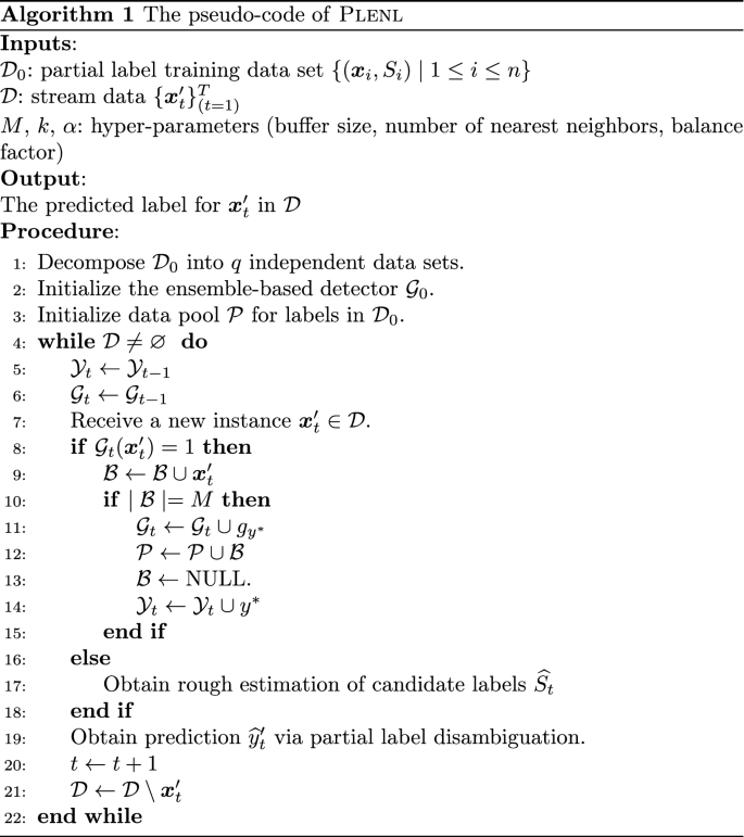
Algorithm 1 presents the pseudo-code of our Plenl approach. As we can see, the model updating process is presented in line 10 to 15. The updating of detection and classification module involves adding a new one-class SVM as base classifier and integrating a few instances from new label into the data pool respectively. In the end of each period, the data will be classified via label disambiguation as shown in line 19.

4 Experiments

4.1 Experimental setup

4.1.1 Data sets

To validate the effectiveness of the proposed method Plenl, we conduct experiments on 9 data sets with different scales. Table 1 summarizes the characteristics of these data sets. Specifically, the first 6 data sets are from UCI repository and the last 3 ones are real-world partial label data sets. For the UCI data sets, we transform them into synthetic partial label data sets by randomly assigning a candidate label set for each instance. In our experiment, the size of candidate label set is set to 2 for all synthetic partial label data sets.

Table 1 Characteristics of the experiment data sets

For each data set in Table 1, the labels are randomly splited into the known labels in the initial data $\mathcal {D}_0$ and the emerging labels in the data stream $\mathcal {D}$. The initial label number q in $\mathcal {D}_0$ for each data set is chosen according to the size of label space, as shown in Table 1. Note that the minimum value of q is set to 3, otherwise the label information of instances in $\mathcal {D}_0$ would be completely eliminated. For the initial known labels, there will be 90% instances presented in $\mathcal {D}_0$, while the rest 10% instances will be randomly distributed in the following periods and mixed with the instances from the new labels with a completely random manner. Furthermore, only one new label $y^*$ emerges in each period, and the detected new label would be regarded as a known one in the next period. To guarantee that there are sufficient instances from each label in all periods, we discard the labels from which the number of instances is fewer than 60.

4.1.2 Comparison methods

The problem of multi-class learning with emerging new labels has been widely studied (Mu et al. 2017b; Zhu and Li 2020; Mu et al. 2017a), however, to the best of our knowledge, there is no work investigating the problem of partial label learning with emerging new labels. Therefore, to compare with the existing methods, we need to firstly transform the initial partial label data sets into the regular multi-class data sets by label disambiguation before employing these methods. Here we employ IPAL, which has been validated as an effective disambiguation method (Zhang and Yu 2015), to conduct label disambiguation. In our experiments, we consider three methods used for multi-class learning with emerging new labels for comparison:

• SENC-Mas (Mu et al. 2017b) utilizes two low-dimensional matrix sketches to detect new labels and classify known labels.

• SENCForest (Mu et al. 2017a) employs completely random trees, which have been shown to work well in unsupervised learning and supervised learning independently in the literature, to perform new label detection and classification.

• SEEN (Zhu and Li 2020) uses a tree-based method for new label detection and an online label propagation method for classification.

Except these methods, we also consider the combinations of anomaly detection and traditional multi-class classification as the baselines:

• iForest (Liu et al. 2008; Chang and Lin 2011) is an unsupervised anomaly detection method based on forest, which will be used to detect new labels. In addition, SVM will be used as the classifier.

• LOF (Breunig et al. 2000) is a commonly used unsupervised anomaly detection method based on local density, which will be used as new label detector. In addition, kNN is used as classifier.

• iNNE (Bandaragoda et al. 2018) is an improved method based on isolation, which can effectively detect the clustering anomaly data and scattered anomaly points, then kNN is used for classification.

• OC-SVM (Ma and Perkins 2003) constructs a hyper-sphere surrounding all instances from known labels to detect new labels. In addition, SVM is used to perform classification.

Table 2 Classification accuracy (mean±std) of Plenl and comparing methods on synthetic partial label data sets

To evaluate the performance of Plenl, we calculate the accuracy on the entire data stream as well as the accuracy on instances up to time t, where the former one indicates the overall performance and the latter one measures the dynamic performance during different periods. We also make a comparison on the time spent for the data stream, shown in Table 5.

Table 3 Classification accuracy (mean±std) of Plenl and comparing methods on synthetic partial label data sets

Fig. 2

The performance changing during stream classification of Plenl and comparing methods on synthetic partial label data sets

4.2 Experimental results

In our method, we simply set $M=250$, $k=10$ and $\alpha =0.9$ on all data sets. For the base classifier one-class SVM, we use RBF kernel function to deal with nonlinear cases. The experiments on each data set are repeated 10 times with different data streams. The mean and standard variance of accuracy on entire data stream are reported in Tables 2, 3 and 4, and the changing of accuracy during periods is presented in Figs. 2 and 3. Except the above mentioned measures, we further evaluate the percentage of new label instances misclassified in the normal class, which is noteds as MissNew, and the results are presented in Tables 6, 7 and 8.

4.2.1 Overall performance

Controlled UCI Data Sets. The results reported in Tables 2 and 3 show the effectiveness of our method. Compared with the methods that focus on multi-class learning with new labels, Plenl achieves superior performance on all cases. Compared with the methods that directly combine anomaly detection and classification, Plenl achieves significantly superior performance on all synthetic partial label data sets except Pendigits, on which LOF outperforms our method with 1%.

Table 4 Classification accuracy (mean±std) of Plenl against comparing methods on real-world partial label data sets

Fig. 3

The performance changing during stream classification of Plenl and comparing methods on real-world partial label data sets

Real-World Data Sets. The results on real-world partial label data sets are reported in Table 4. As we can see, Plenl also achieves superior performance on the real-word partial label data sets against comparing methods, which further validate the effectiveness of our method.

Overall, our method outperforms the others with large margin. Specifically, the average accuracy of our method on all the 9 data sets is 59.5%, which is significantly higher than the best among the rest methods, i.e., 43.9% achieved by iNNE.

Table 5 Runtime (S) of Plenl against comparing methods

Fig. 4

The parameter sensitivity analysis for M, k and $\alpha$. (a): Classification accuracy with different buffer size M in Plenl on BirdSong, Segment, Usps, Mirflickr and Letter; (b-f): Classification accuracy of Plenl with changing k and $\alpha$ on BirdSong, Segment, Usps, Mirflickr and Letter respectively

4.2.2 Performance Changing on Stream

In Figs. 2 and 3, we present the accuracy on data stream during the dynamic learning process. From the results on both synthetic and real-world partial label data sets, we can see that as the instances continuously arrive, the performance margin between our method and the comparing methods will become larger. The improvement of our method can be owed to two perspectives. Firstly, the training of our method is more stable compared with other methods when new labels emerge in the data stream, and this stability makes our method outperform the others after a few initial periods. Another important observation is that our method achieves more significant performance rising after each model updating process, which means that the detection of new labels of our method is more accurate than other methods. Furthermore, we compare the time cost to handle the data stream for different methods, shown in Table 5. As can be observed, compared with other comparing algorithms, Plenl achieves a much better trade-off between time and performance.

4.2.3 Sensitivity analysis

Our method Plenl is instantiated with parameters M, which is employed to control the capacity of the instance buffer. Furthermore, k and $\alpha$ are used to determine the number of neighbors and adjust the label propagation in classification. Figure 4 illustrates how the performance of Plenl changes under different configurations of M, k and $\alpha$.

In Fig. 4a, we observe that the performance of Plenl increases when M varies from 50 to 250 and tends to be stable as M continues to increase. In Fig. 4b, c, d, e and f, $\alpha$ increases from 0.05 to 0.95 with step size 0.1, while k changes from 1 to 19 with step size 2. It is shown that the performance of Plenl is stable across different selections of k, and the best value for $\alpha$ is between 0.5 and 0.95.

Table 6 Evaluation on MissNew (mean±std) of Plenl and comparing methods on real-world partial label data sets.

Table 7 Evaluation on MissNew (mean±std) of Plenl and comparing methods on synthetic partial label data sets.

4.2.4 New label detection analysis

MissNew measures the percentage of new label instances misclassified into the known label set, which is equal to the ratio between the total number of instances from new labels classified into the normal labels and the total number of instances from the new labels in the stream. As shown in Tables 6, 7 and 8, the results validate the effectiveness of our method on new label detection for real-world data sets and controlled UCI data sets. Compared with the other methods, including previous methods for multi-class learning with new labels and combination of anomaly detection and multi-class classifier, Plenl achieves superior performance on all data sets, and it exceeds those methods with large margins.

Table 8 Evaluation on MissNew (mean±std) of Plenl and comparing methods on synthetic partial label data sets.

5 Conclusion

In this paper, partial label learning with emerging new labels is investigated for the first time, and a novel approach Plenl is proposed to address this problem. Plenl employs an ensemble-based detector to identify instances of new labels, while this detector also produces a rough estimation of candidate label set for each instance in data stream. Then, the classification is solved by constructing a data pool to store a small proportion of the previous data and using a graph-based manifold consistency mechanism to disambiguate the labels. In our approach, the detection and classification modules are continuously updated with the emergence of new labels, and this process can be efficiently achieved. Extensive experiments on real-world and controlled UCI data sets validate the effectiveness of the proposed approach.

References

Akoglu, L., Tong, H. H., & Koutra, D. (2015). Graph based anomaly detection and description: A survey. Data Mining and Knowledge Discovery, 29(3), 626–688.
Bai YB, Liu TL (2021) Me-momentum: Extracting hard confident examples from noisily labeled data. In: Proceedings of the IEEE/CVF international conference on computer vision, pp 9312–9321.
Bandaragoda, T. R., Ting, K. M., Albrecht, D., et al. (2018). Isolation-based anomaly detection using nearest-neighbor ensembles. Computational Intelligence, 34(4), 968–998.
Breunig MM, Kriegel HP, Ng RT, et al (2000) LOF: Identifying density-based local outliers. In: proceedings of the ACM SIGMOD international conference on management of data, pp 93–104.
Chandola, V., Banerjee, A., & Kumar, V. (2009). Anomaly detection: A survey. ACM Computing Surveys, 41(3), 1–58.
Chang, C. C., & Lin, C. J. (2011). Libsvm: A library for support vector machines. ACM Transactions on Intelligent Systems and Technology, 2(3), 27–54.
Chen, C. H., Patel, V. M., & Chellappa, R. (2017). Learning from ambiguously labeled face images. IEEE Transactions on Pattern Analysis and Machine Intelligence, 40(7), 1653–1667.
Cour, T., Sapp, B., & Taskar, B. (2011). Learning from partial labels. The Journal of Machine Learning Research, 12, 1501–1536.
Da Q, Yu Y, Zhou ZH (2014) Learning with augmented class by exploiting unlabeled data. In: proceedings of the twenty-eighth AAAI conference on artificial intelligence, pp 1760–1766.
Feng, L., Lv, J. Q., Han, B., et al. (2020). Provably consistent partial-label learning. Advances in Neural Information Processing Systems, 33, 1–26.
Foulds, J., & Frank, E. (2010). A review of multi-instance learning assumptions. The Knowledge Engineering Review, 25(1), 1–25.
Gong, C., Liu, T. L., Tang, Y. Y., et al. (2017). A regularization approach for instance-based superset label learning. IEEE Transactions on Cybernetics, 48(3), 967–978.
Hu XT, Tang KH, Miao CY, et al (2021) Distilling causal effect of data in class-incremental learning. In: proceedings of the IEEE/CVF conference on computer vision and pattern recognition, pp 3957–3966.
Jin, R., & Ghahramani, Z. B. (2002). Learning with multiple labels. Advances in Neural Information Processing Systems, 15, 897–904.
Liu FT, Ting KM, Zhou ZH (2008) Isolation forest. In: eighth IEEE international conference on data mining, pp 413–422
Lv JQ, Xu M, Feng L, et al (2020) Progressive identification of true labels for partial-label learning. In: international conference on machine learning, pp 6500–6510.
Ma J, Perkins S (2003) Time-series novelty detection using one-class support vector machines. In: proceedings of the international joint conference on neural networks, pp 1741–1745.
Mancini M, Naeem MF, Yong-Qin X, et al (2022) Learning graph embeddings for open world compositional zero-shot learning. IEEE Transactions on pattern analysis and machine intelligence, in press
Masud, M. M., Gao, J., Khan, L., et al. (2010). Classification and novel class detection in concept-drifting data streams under time constraints. IEEE Transactions on Knowledge and Data Engineering, 23(6), 859–874.
Mu, X., Ting, K. M., & Zhou, Z. H. (2017). Classification under streaming emerging new classes: A solution using completely-random trees. IEEE Transactions on Knowledge and Data Engineering, 29(8), 1605–1618.
Mu X, Zhu FD, Du J, et al (2017b) Streaming classification with emerging new class by class matrix sketching. In: proceedings of the thirty-first AAAI conference on artificial intelligence, pp 2373–2379
Nguyen N, Caruana R (2008) Classification with partial labels. In: proceedings of the 14th ACM SIGKDD international conference on knowledge discovery and data mining, pp 551–559.
Wang DB, Li L, Zhang ML (2019) Adaptive graph guided disambiguation for partial label learning. In: proceedings of the 25th ACM SIGKDD international conference on knowledge discovery and data mining, pp 83–91.
Xia XB, Liu TL, Han B, et al (2021) Sample selection with uncertainty of losses for learning with noisy labels. In: international conference on learning representations
Xu, N., Qiao, C. Y., Geng, X., et al. (2021). Instance-dependent partial label learning. Advances in Neural Information Processing Systems, 35, 1–12.
Yan Y, Guo YH (2020) Partial label learning with batch label correction. In: proceedings of the AAAI conference on artificial intelligence, pp 6575–6582.
Zhang C, Li GR, Xu QQ, et al (2022) Weakly supervised anomaly detection in videos considering the openness of events. IEEE transactions on intelligent transportation systems, in press
Zhang ML, Yu F (2015) Solving the partial label learning problem: An instance-based approach. In: proceedings of the twenty-fourth international joint conference on artificial intelligence, pp 4048–4054.
Zhang, M. L., & Zhou, Z. H. (2013). A review on multi-label learning algorithms. IEEE Transactions on Knowledge and Data Engineering, 26(8), 1819–1837.
Zhou DW, Ye HJ, Zhan DC (2021) Learning placeholders for open-set recognition. In: proceedings of the IEEE/CVF conference on computer vision and pattern recognition, pp 4401–4410.
Zhou, D. Y., Zhang, Z. K., Zhang, M. L., et al. (2018). Weakly supervised POS tagging without disambiguation. ACM Transactions on Asian and Low-Resource Language Information Processing, 17(4), 1–19.
Zhou, Z. H. (2018). A brief introduction to weakly supervised learning. National Science Review, 5(1), 44–53.
Zhu, Y., Ting, K. M., & Zhou, Z. H. (2018). Multi-label learning with emerging new labels. IEEE Transactions on Knowledge and Data Engineering, 30(10), 1901–1914.
Zhu YN, Li YF (2020) Semi-supervised streaming learning with emerging new labels. In: proceedings of the thirty-fourth AAAI conference on artificial intelligence, pp 7015–7022.
Funding
This work was supported by the National Science Foundation of China (62176055).
Author information
Authors and Affiliations
Contributions
X-R Y and M-L Z conceived the basic idea behind the proposed method. X-R Y and D-B W implemented the algorithm and conducted the experiments. All authors contributed to the interpretation of the results and the write-up of the paper.
Corresponding author
Ethics declarations
Conflict of interest
The authors declare that they have no confilict of interest.
Consent to participate
All the authors consent to participate this work.
Consent for publication
All the authors consent to publish this paper.
Ethics approval
We have carefully conducted the ethical review, and do not see any negative ethical impact.
Additional information
Editors: Yu-Feng Li, Prateek Jain.
Publisher's Note
Springer Nature remains neutral with regard to jurisdictional claims in published maps and institutional affiliations.
Rights and permissions
Springer Nature or its licensor holds exclusive rights to this article under a publishing agreement with the author(s) or other rightsholder(s); author self-archiving of the accepted manuscript version of this article is solely governed by the terms of such publishing agreement and applicable law.
About this article
Cite this article
Yu, XR., Wang, DB. & Zhang, ML. Partial label learning with emerging new labels. Mach Learn 113, 1549–1565 (2024). https://doi.org/10.1007/s10994-022-06244-2
Received:
Revised:
Accepted:
Published:
Issue Date:
DOI: https://doi.org/10.1007/s10994-022-06244-2