Abstract
Image processing algorithms on FPGAs have increasingly become more pervasive in real-time vision applications. Such algorithms are computationally complex and memory intensive, which can be severely limited by available hardware resources. Optimisations are therefore necessary to achieve better performance and efficiency. We hypothesise that, unlike generic computing optimisations, domain-specific image processing optimisations can improve performance significantly. In this paper, we propose three domain-specific optimisation strategies that can be applied to many image processing algorithms. The optimisations are tested on popular image-processing algorithms and convolution neural networks on CPU/GPU/FPGA and the impact on performance, accuracy and power are measured. Experimental results show major improvements over the baseline non-optimised versions for both convolution neural networks (MobileNetV2 & ResNet50), Scale-Invariant Feature Transform (SIFT) and filter algorithms. Additionally, the optimised FPGA version of SIFT significantly outperformed an optimised GPU implementation when energy consumption statistics are taken into account.
Find the latest articles, discoveries, and news in related topics.Avoid common mistakes on your manuscript.
1 Introduction
In recent years, real-time vision systems on embedded hardware have become ubiquitous due to the increased need in different applications such as autonomous driving, edge computing, remote monitoring etc. Field-Programmable Gate Arrays (FPGA) offer the speed and flexibility to architect tight-knit designs that are power and resource-efficient. It has resulted in FPGAs becoming integrated into many applications [1]. Often these designs consist of many low to high-level image processing algorithms that form a pipeline [2]. Increasingly the race for faster processing encourages hardware application developers to optimise the algorithms.
Traditionally optimisations are domain agnostic and developed for general-purpose computing. The majority of these optimisations aim to improve throughput and resource usage by increasing the number of parallel operations [3], memory bandwidth [4] or operations per clock cycle [5]. On the contrary, domain-specific optimisations are more specialised in a particular domain and can potentially achieve larger gain both in terms of faster processing and reducing power consumption. This paper proposes domain-specific optimisation techniques on FPGAs that exploit the inherent knowledge of the image processing pipeline.
Optimisations can be divided into two categories: general-purpose and domain-specific. In image processing, domain-specific optimisations enable a significant reduction of computational load while maintaining sufficient accuracy. Example, optimisations are down-sampling [6], approximation[7], data-type conversion [8], kernel size [9], bit-width [10] and removing operations entirely. Although optimisations of algorithms on hardware accelerators, both in CPU, GPU and FPGAs have been extensively researched in [11,12,13], they are only aimed at the target algorithms. On contrary, there has been very little work on domain-specific optimisations of imaging algorithms on FPGAs. Qiao et al. [14] proposed a minimum cut technique to search fusible kernels recursively to improve data locality. Rawat et al. [15] proposed multiple tiling strategies that improved shared memory and register resources. However, such papers propose constrained domain-specific optimisation strategies that exclusively target CPU and GPU hardware only. Reiche et al. [16] proposed domain knowledge to optimise image processing accelerators using high-level abstraction tools such as domain-specific languages (DSL) and reusable IP-Cores. Other optimisations strategies such as loop unrolling, fission, fusion etc., do not translate well onto FPGA design. In demonstrating our proposition, we present a thorough analysis of well-known image processing algorithms, emerging CNN architectures (MobileNetV2[17] & ResNet50[18]) and Scale Invariant Feature Transform (SIFT) [19]. The decision to select Mobilenet is due to its popular use within embedded systems and ResNet, which consistently obtained higher accuracy rates than other available architectures. In addition, SIFT being the most popular feature extraction algorithm due to its performance and accuracy. The algorithmic properties are exploited with proposed domain-specific optimisation strategies. The optimised design is evaluated and compared with other general optimised hardware designs regarding performance, energy consumption and accuracy. The main contributions of this paper are:
-
Proposition of three domain-specific optimisation strategies for image processing and analysing their impact on performance, power and accuracy; and
-
Validation of the proposed optimisations on a widely used representative image processing algorithms and CNN architectures (MobilenetV2 & ResNet50) through profiling various components in identifying the common features and properties that have the potential for optimisations.
2 Domain-Specific Optimisations
Image processing algorithms typically form a pipeline with a series of processing blocks. Each processing block consists of a combination of low, mid, intermediate and high-level imaging operations starting from colour conversion, filtering to histogram generation, features extraction, object detection or tracking. Any approximation and alteration to the individual processing block or the pipeline have an impact on the final outcome, such as overall accuracy or run-time. However, depending on the applications such alterations are expected to be acceptable as long as they are within a certain error range (e.g., \(\sim \pm 10\%\)).
Many image processing algorithms operations share common functional blocks and features. Such features are useful to form domain specific optimisations strategies. Within the scope of this work, we profile and analyse image processing algorithms to enable potential areas for optimisations. However, such optimisations impact the algorithmic accuracy and therefore it is important to identify the trade-off between performance, power, resource usage and accuracy.
We hypothesise that understanding of this domain knowledge, e.g., processing pipeline, individual processing blocks or algorithmic performance, can be used for optimisations to gain significant improvements in run-time and lower power consumption, especially in FPGA-based resource-limited environments. Based on the common patterns observed in a variety of image processing applications, this section proposes three domain-specific optimisation (DSO) approaches: 1) downsampling, 2) datatype and 3) convolution kernel size. However, on the flip side, often the optimisation can lead to lower accuracy in return for gains in speed and lower energy consumption. We compare the effectiveness of these optimisations against benchmark FPGA, GPU and CPU implementations and show the impact on accuracy. Within the scope of this paper, we have identified three optimisations strategies which are discussed below:
2.1 Optimisation I: Down Sampling
Down/subsampling optimisation reduces the data dimensionality while largely preserving image structure and hence accelerates run-time by lowering the number of computations across the pipeline. Sampling rate conversion operations such as downsampling/subsampling are widely used within many application pipelines (e.g., low bit rate video compression [6] or pooling layers in Convolutional Neural Network (CNN) [20]) to reduce computation, memory and transmission bandwidth. Image downsampling reduces the spatial resolution while retaining as much information as possible. Many image processing algorithms use this technique to decrease the number of operations by removing every other row/column of an image to speed up the execution time. However, the major drawback is the loss of image accuracy due to the removal of pixels. We apply down sampling optimisation using bilinear interpolation and measure both the run-time and accuracy.
2.2 Optimisation II: Datatype
Bit width reduction through datatype conversion (e.g., floating-point (FP) to integer) significantly reduces the number of arithmetic operations resulting in optimised run-time at lower algorithmic accuracy. Whilst quantising from FP to integer representations is a common in the software domain, one of the advantages of reconfigurable hardware is the capability to reduce dimensionality to arbitary sizes (e.g., 7, 6, 5, 4 bits) as a tradeoff between accuracy and power/performance[21,22,23,24].
In the field of Image processing, majority of the algorithms are inherently developed using FP calculations. Although, FP has a higher accuracy representation, it is more expensive to compute, i.e., large number of arithmetic computations resulting in increasing resource (higher bit-width) and energy usage. The substitute for floating-point is fixed-point arithmetic, in which there is a fixed location of the point separating integers from fractional numbers. However, using fixed-point representation, while gaining performance in speed, will result in loss of accuracy vs FP representation. A datatype conversion optimisation is proposed here where all operation stages are converted from FP to integer and note the impact on performance and accuracy.
2.3 Optimisation III: Convolution Kernel Size
Convolution kernel size optimisation reduces computational complexity, which is directly proportional to the squared size of the filter kernel size, i.e., \(\mathcal {O}(n^2)\) or quadratic time complexity. Convolution is a fundamental operation used in most image processing algorithms that modify the spatial frequency characteristics of an image. Given a kernel and image size \(n \times n\) and \(M \times N\), respectively, it would require \(n^2MN\) multiplications and additions to convolve the image. For a given image, the complexity relies on the kernel size leading to a complexity of \(\mathcal {O}(n^2)\). Reducing kernel size significantly lowers the number of computations, e.g., a \(3\times 3\) kernel replacing \(5 \times 5\) kernel would reduce the computation by a factor of \(\text {x}2.7\). Therefore, we propose this as an ideal target for optimisation i.e., to use a smaller kernel size which is however may come at the cost of accuracy.
3 Case Study Algorithms
In order to apply the optimisations proposed in Section 2, In this section, a brief description of the representative algorithms and architectures which the optimisations selected will be applied:

SIFT Algorithmic Block Diagram.
3.1 SIFT
SIFT [19] is one of the widely used prototypical feature extraction algorithms. To demonstrate the proposed optimisations, we’ve implemented various versions of SIFT which consists of two main and several sub-components as shown in Fig. 1 and described below.

a Scale-Space Hardware Block Diagram b Extrema Detection in Local Space/Scale Neighbourhood.
3.1.1 Scale-Space Construction
Gaussian Pyramid
The Gaussian pyramid \(L(x,y,\sigma )\) is constructed by taking in an input image I(x, y) and convolving it at different scales with a Gaussian kernel \(G(x,y,\sigma )\):
where \(\sigma\) is the standard deviation of the Gaussian distribution. The input image is then halved into a new layer (octave), which is a new set of Gaussian blurred images. The number of octaves and scales can be changed depending on the requirements of the application.
The implemented block design reads pixel data of input images into a line buffer show in Fig. 2a. The operations in this stage are processed in parallel for maximum throughput. This is due to significant matrix multiplication operations which greatly impacts the run-time. This stage is the most computationally intensive, making it an ideal candidate for optimisation.
The Difference of Gaussian \({DOG}(x,y,\sigma )\), in Eq.3 is obtained by subtracting the blurred images between two adjacent scales, separated by the multiplicative factor k.
The minima and maxima of the DOG are detected by comparing the pixels between scales shown in Fig. 2b. This identifies points that are best representations of a region of the image. The local extrema are detected by comparing each pixel with its 26 neighbours in the scale space. (8 neighbour pixels within the same scale, 9 neighbours within the above/below scales). Simultaneously, the candidate keypoints with low contrast or located on an edge are removed.
3.1.2 Descriptor Generation
Magnitude & Orientation Assignment
Inside the SIFT descriptor process shown in Fig. 3, the keypoint’s magnitude and orientation are computed for every pixel within a window and then assigned to each feature based on local image gradient. Considering L is the scale of feature points, the gradient magnitude m(x, y) and the orientation \(\theta (x,y)\) are calculated as:
Once the gradient direction is obtained from the result of pixels in the neighbourhood window, then a 36 bin histogram is generated. The magnitudes are Gaussian weighted and accumulated in each histogram bin. During the implementation, m(x, y) and \(\theta (x,y)\) are computed based on the CORDIC algorithm [25] in vector mode to map efficiently on an FPGA.

Magnitude & Orientation Assignment and Keypoint Descriptor Generation.
3.1.3 Keypoint Descriptor
After calculating the gradient direction around the selected keypoints, a feature descriptor is generated. First, a \(16\times 16\) neighbourhood window is constructed around a keypoint and then divided into sixteen \(4\times 4\) blocks. An 8-bin orientation histogram is computed in each block. The generated descriptor vector consists of all histogram values resulting in a vector of \(16 \times 8 = 128\) numbers. The 128-dimensional feature vector is normalised to make it robust from rotational and illumination changes.
3.2 Digital Filters
Digital filters are a tool in image processing to extract useful information from noisy signals. They are commonly used for tasks such as smoothing, edge detection, and feature extraction. Filters operate by applying a kernel, or a small matrix of values, to each pixel of an image. The kernel is convolved with the image, and the resulting output value is placed in the corresponding pixel location of the output image shown in the Eq. 6. Where I(x, y) is the input image and \(K(k_x,k_y)\) is the kernel. The convolution result O(x, y) is calculated by:
The indices \(k_x\) and \(k_y\) correspond to the coordinates of the kernel K, x and y correspond to the coordinates of the output image O.
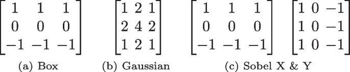
Common image filter kernels
3.2.1 Box
The box filter is a simple spatial smoothing technique that convolves the image with the kernel shown in Fig. 4a, replacing each pixel value with the average of its neighboring pixels. This process has the effect of reducing high frequency noise while preserving the edges and important details of the image. The box filter is also computationally efficient and easy to implement, making it a popular choice for many image processing applications. However, it can cause blurring and loss of sharpness in the image if the kernel size is too large.
3.2.2 Gaussian
The Gaussian filter is a widely used linear filter in image processing and computer vision. It is a type of low-pass filter that removes high-frequency noise while preserving the edges in an image. The filter works by convolving the image with a Gaussian kernel in Fig. 4b, which is a normalised two-dimensional Gaussian distribution. The Gaussian kernel has a circularly symmetric shape and can be expressed mathematically as:
where \(\sigma\) is the standard deviation of the Gaussian distribution, and x and y are the distances from the centre of the kernel. The size of the kernel and the value of \(\sigma\) determine the amount of smoothing applied to the image.
3.2.3 Sobel
The Sobel filter is a type of edge-detection filter that uses two kernels shown in Fig. 4c, one for horizontal changes ( x kernel) and one for vertical changes ( y kernel) in an image. The Sobel filter works by convolving each of these kernels with the image and then computing the gradient magnitude at each pixel using the formula:
where \(G_x\) and \(G_y\) are the convolved images using the x and y kernels, respectively. The resulting gradient image highlights edges in the original image and the direction of the edge can be determined by calculating the angle of the gradient using:
3.3 Convolutional Neural Network
Convolutional Neural Network’s are a class of deep neural networks typically applied to images to recognise and classify particular features. A CNN architecture typically consists of a combination of convolution, pooling, and fully connected layers shown in Fig. 5.

Typical layers implemented within CNN Architectures.
The convolution layers extract features by applying a convolution operation to the input image using a set of learnable filters (also called kernels or weights) designed to detect specific features. The output of the convolution operation is a feature map, which is then passed through a non-linear activation function, such as ReLU, to introduce non-linearity into the network. The convolutional layers can be stacked to form a deeper architecture, where each layer is designed to detect more complex features than the previous one. In addition, it is the most computationally intensive layer because each output element in the feature map is computed by repeatedly taking a dot product between the filter and a local patch of the input, which results in a large number of multiply-add operations.
The pooling layers are responsible for reducing the spatial size of the feature maps while retaining important information. The most common types of pooling are max pooling and average pooling. These layers typically use a small window that moves across the feature map and selects the maximum or average value within the window. This operation effectively reduces the number of parameters in the network and helps to reduce overfitting.
The fully connected layers make predictions based on the extracted features. These layers take the output from the convolutional and pooling layers and apply a linear transformation to the input, followed by a non-linear activation function. The fully connected layer usually has the same number of neurons as the number of classes in the dataset, and the output of this layer is passed through a softmax activation function to produce probability scores for each class. A CNN architecture also includes normalisation layers such as batch normalisation, dropout layers that are used to regularise the network and reduce overfitting, and an output layer that produces the final predictions.
4 Experimental Results and Discussion
We verify the proposed optimisations on ’SIFT’, ’Box’, ’Gaussian’ and ’Sobel’(in Fig. 6) algorithms, as well as MobileNetV2 and Resnet50 CNN architectures. This is achieved by creating baseline benchmarks on three target hardware CPU, GPU and FPGA, followed by the realisations of the optimisations individually and combined. The CPU and GPU versions for Filter and SIFT algorithms are implemented using OpenCV [26]. Pytorch library is used to implement CNN architectures and optimisations. Additionally, both architectures are pre-trained on the image-net classification dataset. The FPGA implementation for all algorithms is developed using Verilog (SIFT/Filter) and HLS (CNN). All baseline algorithms and CNN model use floating point 32 (FP32), and an uncompressed grayscale 8-bit \(1920\times 1080\) input image is used for the SIFT algorithm, and each sub-operation is profiled. Details of the target hardware/software environments and power measurement tools are given in Table 1.
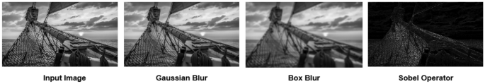
Filter Algorithms Applied onto Input Image.
Dataset
The input images used in the CNN and Filter experiments are from LIU4K-v2 dataset [31]. The dataset contains 2000 high resolution \(3840\times 2160\) images with various backgrounds and objects.
4.1 Performance Metrics
As part of the evaluation process, we measure using three different performance metrics, namely, 1) execution time, 2) energy consumption and 3) accuracy.
4.1.1 Execution Time
The execution time measured for the CPU and GPU platforms uses time function libraries to count the smallest tick period. Each algorithm/operation is run for 1000 iterations and averaged to minimise competing resources or other processes directly affecting the architecture, especially for the CPU architecture. The GPU has an initialisation time which is taken into account and removed from the results. The timing simulation integrated into Vivado design suite software is used to measure the time for the FPGA platform. The experiments exclude the time of both the image read and write from external memory. We compute the frame per second (FPS) as the inverse of the execution time:
4.1.2 Power Consumption
Two common methods used for measuring power are software and hardware-based. Accurately estimating power consumption is a challenge using software-based methods, which have underlying assumptions in their models and may not measure other components within the platform. In addition, taking the instantaneous watt or theoretical TDP of a device is not accurate since power consumption varies on the specific workload. Therefore, we obtain the total energy consumed by measuring the power over the duration of the algorithm executed. A script is developed to automatically start and stop the measurements during the execution of the algorithm and extract the power values from the software.
With the use of a power analyser within the Vivado design suite and the MaxPower-tool, we measure the FPGA power consumption in two parts, (1) static power and (2) dynamic power. Static power relates to the consumption of power when there is no circuit activity and the system remains idle. Dynamic power is the power consumed when the design is actively performing tasks. The power consumption for the CPU and GPU is obtained using HWMonitor and Nvidia-smi software. To have a fair comparison across the target hardware for the SIFT algorithm, we normalise it as the energy per operation (EPO):
Additionally, We calculate the energy consumption for the Filter and CNN algorithms:
4.1.3 Accuracy
With an expectation that the optimisations impact overall algorithmic accuracy, we capture it by measuring the Euclidean distance between the descriptors generated from the CPU (our comparison benchmark) to the descriptor output produced by the FPGA. The Euclidean distance d(x, y) is calculated in Eq. 13 where x and y are vectors, and K is the number of keypoints generated.
Subsequently, the accuracy for each Euclidean distance is calculated using Eq. 14:
The Euclidean Distance denotes the distance between the two descriptor vectors being compared, and Max Distance represents the maximum Euclidean distance found in the vector. The accuracy is transformed to have 100% indicate identical descriptors, while 0% indicates completely dissimilar descriptors.
We used root mean square error (RSME) to compare the input image to the output images produced by each hardware accelerator to determine the pixel accuracy. RMSE is defined as:
Where the difference between the pixel intensity values of output and input (yi,xi) images. Divided by N, which is the total number of pixels in the image.
The accuracy of the CNN architecture is measured by taking the number of correct predictions divided by the total number of predictions:
A high accuracy indicates that the model is making accurate predictions, while a low accuracy suggests room for improvement in the model’s performance.
4.2 Results and Discussions
The results and discussions section contains the evaluation of algorithms in three categories, feature extraction algorithms (SIFT), filter algorithms (Box, Gaussian, Sobel) and Convolution Neural Networks (MobilenetV2, Resnet50).
4.2.1 SIFT
We obtain results for FPGA implementations of the SIFT algorithm, considering various optimisations or combinations of them. Two sets of results are captured for octave, scale of (2,4) and (4,5) as they are regularly reported in the literature for SIFT implementation on FPGA. The results are primarily obtained at a target frequency of 300 MHz for various components of SIFT and execution time and accuracy are reported in Table 2 along with FPS numbers in Fig. 7. Finally, for the completeness we report the resource and power usage statistics for optimised configurations at 300 MHz in Table 3.

SIFT: FPS and Accuracy for each optimisation on both configurations (octave, scale).
In terms of individual optimisations on the base FPGA implementation, down sampling and integer optimisations had the most reduction of accuracy but in trade for a greater reduction of run-time. On the other hand, \(3\times 3\) kernel size (down from default \(5\times 5\)) had better accuracy results but with a small improvement on the overall run-time. In the case of combined optimisations, both down sampling and integer combinations greatly reduced the execution times but at a cost of \(8\sim 10\%\) accuracy loss. In the most optimised case, (4,5) and (2,4) configurations achieved 17 and 50 fps, at an accuracy of \(90.18\%\) and \(89.45\%\), respectively. The \(10 \sim 11\%\) loss in accuracy in both configurations can be attributed to the loss of precision and pixel information resulting in imperfection in feature detection Fig. 7.
The comparison with optimised CPU and GPU implementations are shown in Table 4 which includes total execution time as well as energy consumption per operation (nJ/Op). Results indicate the optimised FPGA implementation achieved comparable GPU run-time at 600 MHz but significantly outperformed them when energy consumption statistics are taken into account. The GPU results excluded the initialisation time, which would add greater latency to the overall run-time. In addition, the power consumption of the GPU is at 12.47nJ/Op, which would make it a difficult choice for real-time embedded systems. On the other hand, optimised FPGA implementations have better performance per watt than the GPU and CPU. The comparison with the state-of-the-art FPGA implementations are reported in Table 5 and results show major improvements in the run-time even with larger image size and more or similar feature points (\(\sim 10000\)).
4.2.2 Filter Implementations
Figures 8 and 9 plots the run-time and energy consumption of three image processing filter algorithms (Box, Gaussian, and Sobel) with various optimisations applied to the baseline algorithm. Comparing the baseline performance, the CPU architecture suffers the most in execution time and energy consumption which can be attributed to lack of many compute cores. In contrast, GPUs and FPGAs exploit data parallelism and stream processing to significantly reduce runtime.

Filter: Runtime comparison for optimisations applied on each architecture.

Filter: Energy consumption comparison for optimisations applied on each architecture.
The figures show that the performance of both GPU and FPGA are comparable in both metrics studied. The GPU demonstrated a marginally better computation speed compared to the FPGA, with a average improvement of \(12.59\%\) for Box and Gaussian algorithms. However, the GPU has been observed to consume \(\sim 1.20\times\) more Joules than the FPGA. The high energy cost can be derived from the support/unused logic components consuming static power. In the case for Sobel, the FPGA is \(1.11\sim 1.5\times\) faster over the GPU across all optimisation strategies. The smaller kernel size allows the FPGA use its DSP slices to efficiently compute the algorithm, whilst the GPU operations do not fully occupy the compute resources available which results in load imbalance and communication latency.
All optimisations, e.g Datatype, Kernel, and Downsampling optimisations had major improvements for each accelerator. Reducing the kernel size to \(3\times 3\) kernel size had the most impact due to lowering the number of operations computed during the convolution operation. The Downsampling and Datatype optimisations had around \(11.8\sim 24.5\%\) decrease in run-time for all algorithms. The optimisation runtime results and accuracy’s of each filter algorithm are reported in Tables 6 and 7 respectively.
4.2.3 CNN Architecture
Figure 10 displays the runtime performances and classification accuracy of the baseline and optimised CNN algorithms on each hardware architecture. The results show that the CPU, GPU, and FPGA exhibit similar levels of performance, with the GPU having an average improvement of \(5.41\sim 12\%\) over the FPGA for the Downsampling optimisation in MobileNetV2 and the baseline for Resnet50, respectively. The FPGA leads in the Datatype optimisation over the GPU with a \(6.25-11.1\%\) reduction in time for both CNNs. The Datatype optimisation involves quantisation of the model’s weights from FP32 to 8-bit to reduce complexity. The FPGA computes the quantised operations faster on both architectures due to exploiting the DSP blocks and requiring no additional hardware logic for floating-point arithmetic. However, the quantised model weights are unable to represent the full range of values present in the input image, resulting in a \(\sim 10\%\) accuracy loss for all platforms. The Downsampling strategy has a slight improvement in run-time with minimal impact on the accuracy, with a loss around \(\sim 5\%\).

CNN: Architecture Execution Time and Classification Accuracy comparison of Model Datatype & Input Image Downsampling Optimisations on Resnet50 and MobilenetV2.

CNN: Architecture Energy comparison of Model Datatype & Input Image Downsampling Optimisations on Resnet50 and MobilenetV2.
In Figure 11, the energy consumption graph shows that the CPU consumes on average \(3.14\times\) more energy than the other accelerators for both CNNs. In addition, the Resnet50 architecture has more layers than MobileNetV2, therefore contains more operations, resulting in higher energy usage. In all cases, the FPGA consumes the least amount of energy, \(1.11\sim 3.55\times\) less than the CPU and GPU, to compute the image classification. The results show the potential of reducing the computation time of CNN’s by further applying particular optimisations in each layer but at the cost of slight accuracy loss. The optimisation results of each CNN architectures and accuracy’s are reported in Table 8.
Consequently, larger images or complex networks with many layers and larger filter sizes require more memory to store the weights and activation’s. This leads to higher memory requirements, especially within real-time embedded systems where space is limited. However, applying optimisations can alleviate the computational load but careful consideration must be taken to understand the trade-offs between runtime and accuracy depending on the application.
5 Conclusion and Future Direction
This paper proposes new optimisation techniques called domain specific optimisation for real-time image processing on FPGAs. Common image processing algorithms and their pipelines are considered in proposing such optimisations, which include down/subsampling, datatype conversation and convolution kernel size reduction. These were validated on the popular image processing algorithms and convolution neural network architectures. The optimisation results for CNN and Filter algorithms vastly improved the computation time for all processing architectures. The SIFT algorithm implementation results significantly outperformed state-of-the-art SIFT implementations on FPGA and achieved run-time at par with GPU performances but with lower power usage. However, the optimisations on all algorithms come at the cost of \(\sim 5-20\%\) accuracy loss.
The results demonstrate that applying domain-specific optimisations to increase computational performance while minimising accuracy loss demands in-depth and thoughtful consideration. One proposal for algorithms comprising multiple operation stages is to use adaptive techniques instead of fixed integer downsampling factors, bit-widths, and kernel sizes, is to employ adaptive techniques. These adaptive methods analyse the data and dynamically adjust the level of optimisation based on input characteristics. For instance, adjusting the bit-width and downsampling factor according to the specific input data within each stage can yield better results and strike a more suitable trade-off between performance and accuracy. Several strategies can be employed in the CNN domain to address the challenges. Quantisation-Aware Training (QAT) and mixed-precision training enable the model to adapt to lower precision representations during training, reducing accuracy loss during inference with quantised weights and activations. Additionally, selective downsampling and kernel size reduction of CNN architectures help retain relevant information and preserve accuracy. Channel pruning can further offset accuracy loss by removing redundant or less critical channels. As a result, employing these strategies and considering hardware constraints makes it possible to strike an optimal balance between accuracy and performance, unlocking the full potential of efficient applications.
On the other hand, the drawback of traditional libraries and compilers is that they often struggle to keep pace with the rapid development of deep learning (DL) models, leading to sub-optimal utilisation of specialised accelerators. To address the limitation, adopting optimisation-aware domain-specific languages, frameworks, and compilers is a potential solution to cater to the unique characteristics of domain algorithms (e.g., machine learning or image processing). These tool-chains would enable algorithms to be automatically fine-tuned, alleviating the burden of manual domain-specific optimisation.
Data Availibility Statement
The datasets generated during and/or analysed during the current study are available from the corresponding author on reasonable request.
References
Bhowmik, D., & Appiah, K. (2018). Embedded vision systems: A review of the literature. In: International Symposium on Applied Reconfigurable Computing, pp. 204–216. Springer.
Liu, H., & Yu, F. (2016). Research and implementation of color image processing pipeline based on FPGA. In: 2016 9th International Symposium on Computational Intelligence and Design (ISCID), 1, 372–375. https://doi.org/10.1109/ISCID.2016.1092
Vourvoulakis, J., Kalomiros, J., & Lygouras, J. (2016). Fully pipelined FPGA-based architecture for real-time SIFT extraction. Microprocessors and Microsystems, 40, 53–73. https://doi.org/10.1016/j.micpro.2015.11.013
Chaple, G., & Daruwala, R. D. (2014). Design of Sobel operator based image edge detection algorithm on FPGA. In: 2014 International Conference on Communication and Signal Processing, pp. 788–792. https://doi.org/10.1109/ICCSP.2014.6949951
Leyva, P., Doménech-Asensi, G., Garrigós, J., Illade-Quinteiro, J., Brea, V. M., López, P., & Cabello, D. (2014). Simplification and hardware implementation of the feature descriptor vector calculation in the SIFT algorithm. In: 2014 24th International Conference on Field Programmable Logic and Applications (FPL), pp. 1–4. https://doi.org/10.1109/FPL.2014.6927409
Lin, W., & Dong, L. (2006). Adaptive downsampling to improve image compression at low bit rates. IEEE Transactions on Image Processing, 15(9), 2513–2521. https://doi.org/10.1109/TIP.2006.877415
Sinha, S., & Zhang, W. (2016). Low-power FPGA design using memoization-based approximate computing. IEEE Transactions on Very Large Scale Integration (VLSI) Systems, 24(8), 2665–2678. https://doi.org/10.1109/TVLSI.2016.2520979
Zeng, Y., Cheng, L., Bi, G., & Kot, A. C. (2001). Integer dcts and fast algorithms. IEEE Transactions on Signal Processing, 49(11), 2774–2782. https://doi.org/10.1109/78.960425
Niklaus, S., Mai, L., & Liu, F. (2017). Video frame interpolation via adaptive separable convolution. In: 2017 IEEE International Conference on Computer Vision (ICCV), pp. 261–270. https://doi.org/10.1109/ICCV.2017.37
Wang, J., Lou, Q., Zhang, X., Zhu, C., Lin, Y., & Chen, D. (2018). Design flow of accelerating hybrid extremely low bit-width neural network in embedded fpga. In: 2018 28th International Conference on Field Programmable Logic and Applications (FPL), pp. 163–1636. https://doi.org/10.1109/FPL.2018.00035
Wang, W., Yan, J., Xu, N., Wang, Y., & Hsu, F.-H. (2015). Real-time high-quality stereo vision system in FPGA. IEEE Transactions on Circuits and Systems for Video Technology, 25(10), 1696–1708. https://doi.org/10.1109/TCSVT.2015.2397196
Steinbrücker, F., Sturm, J., & Cremers, D. (2014). Volumetric 3d mapping in real-time on a CPU. In: 2014 IEEE International Conference on Robotics and Automation (ICRA), pp. 2021–2028. https://doi.org/10.1109/ICRA.2014.6907127
Rister, B., Wang, G., Wu, M., & Cavallaro, J. R. (2013). A fast and efficient sift detector using the mobile GPU. In: 2013 IEEE International Conference on Acoustics, Speech and Signal Processing, pp. 2674–2678. https://doi.org/10.1109/ICASSP.2013.6638141
Qiao, B., Reiche, O., Hannig, F., & Teich, J. (2019). From loop fusion to kernel fusion: A domain-specific approach to locality optimization. In: 2019 IEEE/ACM International Symposium on Code Generation and Optimization (CGO), pp. 242–253. https://doi.org/10.1109/CGO.2019.8661176
Rawat, P. S., Vaidya, M., Sukumaran-Rajam, A., Ravishankar, M., Grover, V., Rountev, A., Pouchet, L.-N., & Sadayappan, P. (2018). Domain-specific optimization and generation of high-performance gpu code for stencil computations. Proceedings of the IEEE, 106(11), 1902–1920. https://doi.org/10.1109/JPROC.2018.2862896
Reiche, O., Häublein, K., Reichenbach, M., Schmid, M., Hannig, F., Teich, J., & Fey, D. (2015). Synthesis and optimization of image processing accelerators using domain knowledge. Journal of Systems Architecture, 61(10), 646–658. https://doi.org/10.1016/j.sysarc.2015.09.004
Sandler, M., Howard, A., Zhu, M., Zhmoginov, A., & Chen, L. -C. (2018). Mobilenetv2: Inverted residuals and linear bottlenecks. In: 2018 IEEE/CVF Conference on Computer Vision and Pattern Recognition, pp. 4510–4520. https://doi.org/10.1109/CVPR.2018.00474
He, K., Zhang, X., Ren, S., & Sun, J. (2016). Deep residual learning for image recognition. In: 2016 IEEE Conference on Computer Vision and Pattern Recognition (CVPR), pp. 770–778. https://doi.org/10.1109/CVPR.2016.90
Lowe, D. G. (2004). Distinctive image features from scale-invariant keypoints. International journal of computer vision, 60(2), 91–110.
LeCun, Y., Bottou, L., Bengio, Y., & Haffner, P. (1998). Gradient-based learning applied to document recognition. Proceedings of the IEEE, 86(11), 2278–2324.
Pappalardo, A. Xilinx/brevitas. (2023). https://doi.org/10.5281/zenodo.3333552
Colangelo, P., Nasiri, N., Nurvitadhi, E., Mishra, A., Margala, & M., Nealis, K. (2018). Exploration of low numeric precision deep learning inference using intel®fpgas. In: 2018 IEEE International Symposium on Field-Programmable Custom Computing Machines (FCCM), pp. 73–80. https://doi.org/10.1109/FCCM.2018.00020
Lee, D.-U., Gaffar, A. A., Cheung, R. C. C., Mencer, O., Luk, W., & Constantinides, G. A. (2006). Accuracy-guaranteed bit-width optimization. IEEE Transactions on Computer-Aided Design of Integrated Circuits and Systems, 25(10), 1990–2000. https://doi.org/10.1109/TCAD.2006.873887
Jacob, B., Kligys, S., Chen, B., Zhu, M., Tang, M., Howard, A., Adam, H., & Kalenichenko, D. (2018). Quantization and training of neural networks for efficient integer-arithmetic-only inference. In: 2018 IEEE/CVF Conference on Computer Vision and Pattern Recognition, pp. 2704–2713. https://doi.org/10.1109/CVPR.2018.00286
Andraka, R. (1998). A survey of cordic algorithms for fpga based computers. In: Proceedings of the 1998 ACM/SIGDA Sixth International Symposium on Field Programmable Gate Arrays, pp. 191–200.
Bradski, G. (2000). The OpenCV Library. Journal of Software Tools.
Paszke, A., Gross, S., Massa, F., Lerer, A., Bradbury, J., Chanan, G., Killeen, T., Lin, Z., Gimelshein, N., Antiga, L., Desmaison, A., Kopf, A., Yang, E., DeVito, Z., Raison, M., Tejani, A., Chilamkurthy, S., Steiner, B., Fang, L., Bai, J., & Chintala, S. (2019). Pytorch: An imperative style, high-performance deep learning library. In: Advances in Neural Information Processing Systems 32, pp. 8024–8035. Curran Associates Inc., ???. http://papers.neurips.cc/paper/9015-pytorch-an-imperative-style-high-performance-deep-learning-library.pdf
HWMONITOR. (2023). https://www.cpuid.com/softwares/hwmonitor.html
NVIDIA System Management Interface. (2023). https://developer.nvidia.com/nvidia-system-management-interface
USB-to-PMBus Interface. (2023). https://www.stg-maximintegrated.com/en/products/power/switching-regulators/MAXPOWER.html
Liu, J., Liu, D., Yang, W., Xia, S., Zhang, X., & Dai, Y. (2019). A comprehensive benchmark for single image compression artifacts reduction. In: arXiv.
Chiu, L.-C., Chang, T.-S., Chen, J.-Y., & Chang, N.Y.-C. (2013). Fast SIFT design for real-time visual feature extraction. IEEE Transactions on Image Processing, 22(8), 3158–3167. https://doi.org/10.1109/TIP.2013.2259841
Mizuno, K., Noguchi, H., He, G., Terachi, Y., Kamino, T., Fujinaga, T., Izumi, S., Ariki, Y., Kawaguchi, H., & Yoshimoto, M. (2011). A low-power real-time SIFT descriptor generation engine for full-HDTV video recognition. IEICE Transactions, 94-C, 448–457. https://doi.org/10.1587/transele.E94.C.448
Vourvoulakis, J., Kalomiros, J., & Lygouras, J. (2016). Fully pipelined FPGA-based architecture for real-time SIFT extraction. Microprocessors and Microsystems, 40. https://doi.org/10.1016/j.micpro.2015.11.013
Funding
N/A
Author information
Authors and Affiliations
Contributions
All authors have made substantial contributions to the conception and design of the work.
Corresponding author
Ethics declarations
Ethics Approval
N/A.
Conflict of Interest/Competing Interests
The authors declare that they have no conflicts of interest to report.
Additional information
Publisher's Note
Springer Nature remains neutral with regard to jurisdictional claims in published maps and institutional affiliations.
Rights and permissions
Open Access This article is licensed under a Creative Commons Attribution 4.0 International License, which permits use, sharing, adaptation, distribution and reproduction in any medium or format, as long as you give appropriate credit to the original author(s) and the source, provide a link to the Creative Commons licence, and indicate if changes were made. The images or other third party material in this article are included in the article's Creative Commons licence, unless indicated otherwise in a credit line to the material. If material is not included in the article's Creative Commons licence and your intended use is not permitted by statutory regulation or exceeds the permitted use, you will need to obtain permission directly from the copyright holder. To view a copy of this licence, visit http://creativecommons.org/licenses/by/4.0/.
About this article

Cite this article
Ali, T., Bhowmik, D. & Nicol, R. Domain-Specific Optimisations for Image Processing on FPGAs. J Sign Process Syst 95, 1167–1179 (2023). https://doi.org/10.1007/s11265-023-01888-2
Received:
Revised:
Accepted:
Published:
Issue Date:
DOI: https://doi.org/10.1007/s11265-023-01888-2