Abstract
Recently, correlation filters and deep convolutional network show good performance for visual tracking. Many real-time and high accuracy tracking algorithms are realized; however, there are still some challenges to build a robust tracker. In this paper, we present a novel tracking framework named multi-attention filter (MAF) to solve some challenges for tracking like object drift in a long time, lack of training samples and fast motion. Our framework consists of two components, a basic CNN network to extract feature maps and a set of classifiers to distinguish between the target and the background. First, to solve the problem of object drift in a long time, a simple but effective evaluation mechanism is proposed to the framework, the evaluation mechanism checks the tracking results and corrects it when needed. In addition, the results from different classifiers are fused to predict the object location according to intersection over union. Second, to overcome the lack of training samples, MAF stores some positive and negative samples in two queues, one named long-term queue and another named short-term queue. Third, to deal with fast motion of the target, attention mechanisms including channel attention and location attention are added to the tracker. In our experiments on the popular benchmarks including OTB-2013 and OTB-2015. MFA achieves state of the art among trackers, and as a correlation filter framework, MAF is very flexible and has great rooms for improvement and generalization.
1 Introduction
Visual object tracking is a significant problem in computer vision with a wide range of applications like automatic driving and robotic services. Given the position of object in the first frame, tracking algorithm can capture the object in the video sequences. But there are still lots of challenges and situations for visual tracking to deal with, such as occlusions, fast motion and background interference. Therefore, many attempts have been addressed to how to improve the performance of tracking in recent years.
Recently, two different categories for tracking have emerged. One uses deep network of CNN to train a tracker which benefits from strong recognition ability by CNN model offline on datasets [1,2,3,4,5,6]. The other is correlation filters to train a tracker which benefits from cyclic matrix and online updates to satisfy the real-time requirement [3, 4, 7, 8]. Generally speaking, CNN-based trackers are more robust than correlation filter-based trackers, but correlation filter-based trackers can easily run at real time. Hence, researchers pay more attention to combine them to balance speed and accuracy.
As we know, visual tracking still faces challenging due to many factors. The key to construct a robust tracker is to design a discriminative feature and a powerful classifier. Many researchers combine deep features and handcraft features to form a discriminative feature. As for a powerful classifier, the performance of classifiers depends on the number of training data. Besides, there are still many aspects that can improve tracking performance. For instance, most of trackers only consider the object feature of current frame, which hardly benefit from the motion information from historical frames. The motion information can provide a lot of positive interframe information about tracking task. In order to fit the change of object, most correlation filters algorithms update at each frame, which causes high computational load. At the same time, if we update after in a fixed time, tracking accuracy may decline. Hence, high-quality tracking algorithms remain scarce due to the situations and challenges as mentioned above.
In this paper, we propose a novel framework to form a more robust and more efficient tracker. We independently train a classifier for each channel deep feature. The final response map is produced by fusing all the response maps adaptively. In order to decline the time of update and improve the accuracy, long-term and short-term update strategy (LSUS) and attention mechanisms are introduced into our framework. In conclusion, we have the following contributions:
-
We propose a novel framework named MAF, which train a classifier independently for each channel feature and fuse the response maps adaptively.
-
We utilize location attention to predict location roughly instead of local search or global search to reduce time cost and improve accuracy rate. A long-term and short-term updating strategy can be viewed as a novel update strategy to overcome the occlusion of target and fit appearance change of target.
-
The proposed tracker achieves good performance on OTB-2013 and OTB-2015 [9, 10] benchmarks. Our results show distance precision rate of 86.5% and overlap success rate of 65.7% on OTB-2015.
2 Related work
2.1 Related tracking algorithms
In the following, we will discuss the most related tracking work for recent surveys including deep features, correlation filters and attention mechanisms. Now the mainstream visual tracking algorithm framework is mainly divided into two categories: The first is deep learning-based trackers, and the second is correlation filter-based trackers.
GOTURN [5] uses ALOV300+ video sequence set and ImageNet [2] to train a convolution network based on image pair input. The output is the changes relative to the position of the previous frame in the search area, so as to get the position of the target in the current frame. In order to get the large data set needed for network training, the author not only uses the random continuous frame pairs in the video sequence set, but also uses more single picture sets for data enhancement. CFNet [11] interprets the correlation filter as a differentiable layer in a deep neural network. These approaches advance the development of end-to-end deep tracking models and achieve very good results on recent benchmarks and challenges. Following the end-to-end ideas, a Siamese network is utilized to estimate the similarities between the target in the previous frame and candidate patches [13,12,14,15]. It recently shows good performance in speed to quickly track the target without online fine-turning. Inspired by detection algorithms [6, 16, 17], SiamRPN [18] adopt region proposal network (RPN) to produce a set of candidate regions including regression and classification branch. AlexNet [2] and VGG [19] are used in visual tracking in the past few years and realize good performance. Recently, some deeper network like ResNet-101 shows better performance for tracking task. But there is some weakness. First is training network offline which needs lots of training data. Network generalization ability depends on training data. When the algorithm deals with the object which never met before, it may be fail. Due to too many parameters in network for update, the end-to-end approach does not have an advantage in speed.
Based on correlation filter (CF) methods, CF has shown very popular due to its computation speed [20, 21]. CSK [22] uses a circular matrix for dense sampling to generate a large number of samples with low computational load. CSK introduces kernel space into correlation filter and results in famous kernelized correlation filters (KCF) [3, 4] using histogram of oriented gradients (HOG) [23] handcraft features. However, such an online tracking is easy to drift and fails to follow the target for a long time. This is mainly due to handcraft features. Some approaches improve the trackers by leveraging some stronger features extracted from neural network for a richer representation of the tracking target. As we know, CNN feature is more powerful for tracking task comparing to traditional handcraft features such as HOG [23], SIFI and CN [24, 25]. So many trackers follow the idea that combines deep features with correlation filters like C-COT [22], ECO [26] and CF2. C-COT converts feature maps of different resolutions extracted from different layers of a pretrained CNN model such as VGG into a continuous spatial domain to achieve better accuracy. The subsequent ECO improves the C-COT tracker in terms of performance and efficiency. MHIT [27] efficiently fuses the multi-branch independent solutions of CF via an adaptive weight strategy instead of fusion deep features for more reliable tracking. Attention mechanisms [28] are widely used in natural language processing (NLP). As for computer vision, it is found that the features from different layers have different importance in tracking different objects named channel attention. In contrast to previous deep architectures for tracking, RASNet [14] reformulates the Siamese tracking from a regression prospective and propose a weighted cross-correlation to learn the whole Siamese model from end to end. RASNet includes general attention, residual attention and channel attention to learn deep model to online tracking target (Fig. 1).

Overview of the architecture of our tracking framework. Location attention locates the target according to the law of historical frames roughly. Then, sample densely and sparsely using the heat maps generated by location attention to produce a set of CNN features. After that, we train a filter or classifier for each feature independently. The model online update strategy is LUSU (more details in Sect. 3.3). At last, an adaptive fusion is utilized to produce the final response map
3 Proposed method
3.1 Correlation filter for visual tracking
We choose the discriminative correlation filter-based tracker [20]. Correlation filter (CF) is an important method for tracking task. It comes from the field of signal processing. In signal processing, it is used to measure the difference between two signals. For tracking task, we use it to measure the similarity of the target and search regions. According to the response map, the region with the highest score is chosen to be the prediction location of the target in the next frame. CF tries to learn a model on a set of training data. In Eq. 1, \( f \) is the input image and \( h \) is the filter corresponding to the input.* stands for convolution operation. \( g \) is the response map. Given an example, if you want to track a car in video sequences, the filter can be viewed as the shadow or template of the car, and the goal is to find the most similar part to the template.
To speed up the computing process and reduce the complexity of solving filter template, we can transform the problem into frequency domain by Fourier transform. Correlation filter is computed in the Fourier domain fast Fourier transform (FFT). The 2D Fourier transform of the input image is \( F = {\text{FFT}}\left( f \right) \), and the filter is \( H = {\text{FFT}}\left( h \right) \). Hence, Eq. 1 becomes the form as shown in Eq. 2. The symbol of \( \odot \) denotes element-wise multiplication. Naturally, the Fourier transform of the response map is G = FFT(g). \( * \) indicates the complex conjugate.
Now, the key point is how to find a filter that maps training inputs to the desired training outputs. The objective is to learn the optimal correlation filter H by minimizing the cost function.
where loss function is the sum of squared error between the actual output and the desired output. The desired output is generated from ground true like 2D Gaussian-shaped peak centered on the target. In other words, desired output \( G_{i} \) is the Gaussian response map and the max of response value is in the middle of the object. Of course, regularization term can be added to the loss function to avoid overfitting.
Solving the optimization problem is easy. Let the derivative of \( H^{* } \) be 0. We can get a closed-form expression for \( H^{* } \), as shown in Eq. 4. Given a set of samples \( \left( {G_{i} , F_{i}^{*} } \right) \), Eq. 4 can be used to train our model \( H^{* } \).
3.2 Multi-filters and adaptive fusion mechanism
As mentioned earlier, a representative feature is significant for visual tracking. A representative feature should be discriminative and generalized. Briefly, depending on a single feature to design our trackers is unreliable. Hence, many attempts on features design have shifted from the handcraft features like CN and HOG to CNN features. It is widely understood that, in a deep CNN trained for image classification task, features from deeper layers contain stronger semantic information and are more invariant to object appearance changes. The features from shallow layer have more local location and provide rich detail information.
Through the above discussion, each feature has its limitations.
Some go worse when facing deformation and occlusion [29,30,31]. But some features have better stability when dealing with deformation. However, it is prone to drifting easily when having similar objects. To build a robust tracker, a feature pyramid networks is proposed to fuse all features. During online tracking, the size of the object changes frequently. So in this framework, we utilize independent CNN features and handcraft features to train filters and adaptively combine them. In the next frame, we use multi-filters to enhance robustness of the algorithm and fuse for each response maps to get the final response map.
where \( H_{i}^{*} \) is the filter trained for different features, \( F_{i} \) is the feature vectors extracted from input, \( w^{i } \) is the weight coefficient and \( G \) denotes the final response map in
where \( {\text{FFT}}^{ - 1} \) is inverse Fourier transform and \( g \) is the response map in spatial domain.
There are some details about multiple filters. First, the final location of the object is predicted by intersection over union (IOU). Second, the excessive number of filters will result in the model being too complex and the cost of model updating is too high. So model chooses the top \( N \) with higher-energy filters to represent other filters. Other filters are represented by linear combination of \( N \) filters. \( h \) is the weight coefficient.
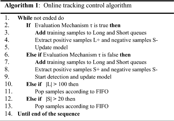
3.3 Long-term and short-term updating strategy and evaluation mechanism
Model updating strategy is also an aspect that can significantly improve the effectiveness. As we know, target is constantly changing and will undergo deformation, occlusion and so on. As a result, the difference between the object and the initial state becomes larger and larger. Hence, the fitting ability of the original model to the object characteristics decreases.
Model updating strategy tries to find a balance between time cost and accuracy. In short, if the model is updated each frame, time cost will be high. On the contrary, if the model is not updated timely according to the latest samples, the model may miss the information of target deformation. In the follow-up video sequences, the target drift may occur. Online update is very necessary comparing with model stable, as shown in Fig. 2.

Use HCF [32] as a tracker to test on OTB2013. Red curve represents model update online, and blue curve represents model stable (color figure online)
Since online update is necessary, how to choose an appropriate update frequency. If update strategy is applied to filter each frame, as shown frame #160 in Fig. 3. Maybe can lead wrong factors into it (Frame #160 #170 may lead “tree” factor into the model in Fig. 3) and cause high computational load. On the contrary, if do not update each frame, maybe cannot adapt to the target appearance change timely (Fig. 4).

A test sequence from OTB dataset. Use one filter to track the target; the ground truth is selected every 10 frames (showing in blue bounding box). As we can see, peak value is greater than threshold (set 0.3) at first. Peak value can measure the similarity between candidate regions and filter template. When the car is occluded by tree in Frame #160, value is lower than threshold (showing in red value), which means the filter is not suitable for the target (color figure online)

Illustration of long-term and short-term updating strategy and evaluation mechanism τ. If the prediction can pass mechanism τ, the training samples come from the queue above the illustration. On the contrary, the training samples come from the queue below the illustration
In tracking control, we adopt long-term and short-term updating strategy. Two sample queues save different training data. One is long-term updating queue, and the other is short-term updating queue.
The positive and negative samples collected dynamically in the previous 100 frames are stored in the long updating queue, and the positive and negative samples collected in the previous 20 frames are stored in the short update queue. The purpose of maintaining two queues is to realize a longtime tracking model. It is widely believed that the performance of the model will be better with the more training data. From this view, we can keep as many old and new samples as possible to train the model. Of course, queue capacity is limited. The model will randomly lose part of the training samples. In addition, we analyze the relationship between peak value and predicted results in depth. Peak value can measure the similarity between candidate regions and filter template. Generally speaking, the greater the peak value, the confidence of the prediction result is greater. As mentioned above, if the peak values of most filters are relatively low, there is a reason to believe that the predicted result is unreliable. We can call it evaluation mechanism.
Long-term updates have a fixed frequency, which is the interval of a certain period. In our experiment, we select the update frequency which is 10 frames. Short-term updates only occur in the case of tracking failure. We can assume that when most of peak values are less than the set threshold, tracking failure happens.
Long-term and short-term updates cannot be carried out simultaneously. When the update period is reached and the algorithm can still track the target object successfully, it shows that the change of target and background is not drastic. The ability of model to describe the features of the target object and to distinguish the background and target can still meet the requirement of tracking the target effectively. Although the positive feature samples maintained in long-term queue may be far from the current frame, they conform to the feature distribution of the target object. Therefore, the positive samples in the long queue and the negative samples in the short queue are used as training data to update the model.
Short-term update shows that the target tracking fails and the target object and background change greatly, such as large deformation and occlusion. The model has a serious decline in the ability to express the features of the changed target object. At this time, the feature information maintained in the long-term queue which is far away from the current target object will interfere with the update of the model. When updating, the model is trained by using the positive and negative feature samples of the nearest neighbors maintained in the short-term queue.
Negative samples to train model based on short-term queue maintenance are used for both long-term and short-term updates, which is based on the assumption that the background is constantly changing. Therefore, the background features in the frames with long distances are no longer applicable to the current background. The ultimate goal of online update strategy is to keep the model robust and adaptable to the changing background and target objects (Fig. 5).

A result is shown when use SRDCF [33] as a tracker (shown in red bounding box). Obviously, it is wrong. When adopt our proposed update strategy, SRDCF can adapt some challenged situations (shown in blue bounding box) (color figure online)
3.4 Location attention and channel attention
As we know, candidate regions usually are obtained by dense sampling around the target in the last frame and then take the samples as input to get the response map.
However, it is not suitable for the following situations: Targets move diagonally in the field of view or the distance of targets between two frames is comparable far because the location of the target is not in the region proposals. Naturally, the result is not conceivable. Due to the consistency of motion of objects, if the target moves very slow in the previous frames, we can infer that the target will appear near the location in the last frame. If the target moves very fast in the previous frames, we can infer that the target will appear far away from the location of the target in last frame. MAF considers using optical flow to predict location roughly. MAF can warp motion information to current frame to produce a heat map and then sample densely and sparsely instead of local search or global search.
In the N-channel feature maps extracted by convolution layer, each channel’s feature map corresponds to a specific visual pattern, that is, each channel extracts different information, such as different edges, colors and textures. Therefore, in a specific tracking scene, the contribution of different channels of the feature maps to the measurement of final similarity is different [15, 34,35,36]. Some features are important and some does not play a key role.
Channel attention mechanism can be seen as a process of filtering the semantic attributes of different channels of target template features extracted from convolutional networks. In the process of tracking, when the target object is deformed and occluded, the contribution value of different channel features will change accordingly. Channel attentions are designed to give corresponding weights to different channel features to adapt to the changes of the target object in the process of tracking. Channel attention is also obtained by offline learning of deep neural network in the pretrained stage, but in online tracking, the network only propagates forward without online updating, which is very helpful to improve the tracking speed (Fig. 6).

Dark red, blue and light red indicate different channel attention for tracking different targets (color figure online)
Assume that the features extracted from convolutional networks are Z, where d is the number of channels and \( \beta_{i} \) represents channel attention learned from channel attention network.
4 Experiments
4.1 Implementation details
Our proposed framework is implemented in python, and deep network uses Tensorflow on NVIDIA GTX 1080 GPU. To evaluate the performance of the proposed algorithm in this paper, we choose popular datasets OTB-2013, OTB-2015 and VOT-2016 [37] tracking benchmarks. OTB dataset is the first tracking benchmarks proposed in 2013. OTB-2013 includes 50 video sequences. These sequences are captured in many conditions like occlusion (OCC), deformation (DE), illumination variation (ILV), etc. We use the success plot to evaluate all trackers on OTB dataset, and success rate means the percentage of successfully tracked frames by measuring the overlap score for trackers on each frame. As for VOT-2016, it is similar with ImageNet including 60 color sequences. Each frame is fine marking in VOT-2016. When tracking failure, it will run the platform given the target detection algorithm to detect the object again to run the algorithm. OTB-2015 starting from a random frame, or a rectangle with random disturbance to initialize the tracking algorithm, more in line with the actual situation.
4.2 Evaluation MAF on OTB-2013
Three innovation points are added to fDSST [38]. We set the regularization parameters to 0.1, and the weight of each response maps is consistent with the channel attention because we train a filter for each channel feature. When the channel attention is lower than 0.1, we will ignore it and normalization of fusion weights.
We choose some state-of-the-art trackers to compare MAF including KCF, CNN-SVM, MEEM, MUSTer, DSST, TGPR, SCM, Struck and ours (Fig. 7).

Comparisons with some state-of-the-art trackers on OTB2013 using distance precision rate (DPR) and overlap success rate (OSR)
Our work realizes good performance against all state-of-the-art trackers. As we can see, our work gets 90.9% accuracy rate at 20 pixels (DPR) and overlap success rate (OSR) is 0.678 at 0.6 on OTB2013.
4.3 Evaluation of attention mechanism
We consider adding two attention mechanisms to SiamFC [13] separately. SiamFC use Siamese network to evaluate similarity between target and candidate region. Just like many trackers, candidate regions are produced by sampling around the location in the last frame. Obviously, it is not suitable for fast motion. So we want to use optical flow from previous two frames and then warp it into the current frame. We obtain a heat map which indicates location probability of target occurrence.
Considering the high computational cost of calculating optical flow from pixel to pixel and get the motivation from YOLO, a detection method. We divide the image pairs into 7 * 7 grids; if the center of the target falls into a grid cell, that grid cell is responsible for the target to produce a heat map. As for channel attention, filter coefficients and channel weights are joint-learned to make them optimal. Then, the learned channel weights are viewed as a priori to guide channel weights learning.
Figures 8, 9 and 10 show the effect of three attention mechanisms on OTB-2015 based on SiamFC, PTAV and BACF.

Comparisons with channel attention, location attention and all attention on OTB2015 using distance precision rate (DPR)- and overlap success rate (OSR)-based SiamFC [13] on OTB-2015

We add channel attention and location attention to SiamFC. Comparisons with trackers on OTB2015 using distance precision rate (DPR) and overlap success rate (OSR) on OTB-2015

Detection-based mechanism. When finding an unreliable tracking result (showing red bounding box in b), detection algorithm gives right location (showing blue bounding box in d). In f, we can see detection algorithm gives many bounding boxes, so we choose a best one which is most like positive samples from long-term queue (showing blue bounding box in f) (color figure online)
The precision at 20 pixels for precision plots of basic SiamFC is 0.856, and the area-under-curve score for success plot is 0.643. Location attention can improve 0.58% in DPR and 0.93% in OSR. Channel attention can improve 0.11% in DPR. All attention can improve 1.10% in DPR and 2.20% in OSR.
The precision at 20 pixels for precision plots of basic PTAV is 0.849, and the area-under-curve score for success plot is 0.635. Location attention can improve 0.12% in DPR and 1.89% in OSR. Channel attention can improve 0.02% in DPR and 1.30% in OSR. All attention can improve 1.65% in DPR and 2.52% in OSR.
The precision at 20 pixels for precision plots of basic BACF is 0.822, and the area-under-curve score for success plot is 0.621. Location attention can improve 2.31% in DPR and 2.90% in OSR. Channel attention can improve 2.07% in DPR and 1.61% in OSR. All attention can improve 3.53% in DPR and 1.61% in OSR (Table 1).
4.4 LSUS and evaluation mechanism on OTB-2015
We consider adding long-term and short-term updating strategy to KCF. KCF updates filters each frame, and we add different updating strategy and evaluation mechanisms. KCF is not suitable for longtime tracking, because always wrong information is always introduced in it. In our experiment, we set threshold of peak values is 0.3 and threshold of percentage is 0.8. When the prediction cannot pass evaluation mechanism, we adopt detection algorithm Fast R-CNN to correct location and change training data sources from short-term queue instead of long-term queue (Fig. 11).

Some results are showing (red is ground true, yellow is ours, blue is ECO, purple is KCF, and green is SiamFC) (color figure online)
5 Conclusions
While observing the problems of the existing tracking methods, we have proposed a framework to overcome them. First, long-term and short-term updating strategy (LSUS) as a novel update strategy makes model more flexible to fit some complex scenarios. Second, longtime target tracking is realized by evaluation mechanism. Third, location and channel attention to predict location roughly instead of local search or global search reduce time cost. Our tracking algorithm outperforms the state-of-the-art trackers in terms of both tracking speed and accuracy, in OTB-2013 and OTB-2015 benchmarks. In the future, we plan to continue exploring the effective fusion of deep features in object tracking task.
Change history
10 February 2020
A Correction to this paper has been published: https://doi.org/10.1007/s11760-020-01651-1
References
Xu, T., Feng, Z.H., Wu, X.J., Kittler, J.: Learning adaptive discriminative correlation filters via temporal consistency preserving spatial feature selection for robust visual tracking (2018)
Krizhevsky, A., Sutskever, I., Hinton, G.E.: Imagenet classification with deep convolutional neural networks. In: International Conference on Neural Information Processing Systems, pp. 1097–1105 (2012)
Liang, S., Chen, J.Y., Jin-Liang, W.U., et al.: Long-time video object tracking algorithm based on KCF framework. Radio Commun. Technol. (2017)
Henriques, J.F., Rui, C., Martins, P., et al.: High-speed tracking with kernelized correlation filters. IEEE Trans. Pattern Anal. Mach. Intell. 37(3), 583–596 (2015)
Held, D., Thrun, S., Savarese, S.: Learning to track at 100 fps with deep regression networks, pp. 749–765 (2016)
Redmon, J., Divvala, S., Girshick, R., et al.: You only look once: unified, real-time object detection (2015)
Danelljan, M., Robinson, A., Khan, F.S., Felsberg, M.: Beyond correlation filters: learning continuous convolution operators for visual tracking. In: ECCV (2016)
Lukezic, A., Vojir, T., CehovinZajc, L., Matas, L., Kristan, M.: Discriminative correlation filter with channel and spatial reliability. In: The IEEE Conference on Computer Vision and Pattern Recognition (CVPR) (2017)
Wu, Y., Lim, J., Yang, M.-H.: Online object tracking: a benchmark. In: Proceedings of the IEEE Conference on Computer Vision and Pattern Recognition, pp. 2411–2418 (2013)
Dalal, N., Triggs, B.: Histograms of oriented gradients for human detection. In: IEEE Computer Society Conference on Computer Vision and Pattern Recognition, 2005. CVPR 2005, vol. 1, pp. 886–893. IEEE (2005)
Danelljan, M., Hager, G., Shahbaz Khan, F., et al.: Learning spatially regularized correlation filters for visual tracking. In: Proceedings of the IEEE International Conference on Computer Vision, pp. 4310–4318 (2015)
Zhu, Z., Wang, Q., Li, B., Wu, W., Yan, J., Hu, W.: Distractor-aware siamese networks for visual object tracking. In: European Conference on Computer Vision, pp. 103–119. Springer (2018)
He, A., Luo, C., Tian, X., et al.: A twofold siamese network for real-time object tracking (2018)
Wang, Q., Teng, Z., Xing, J., Gao, J., Hu, W., Maybank, S.: Learning attentions: residual attentional siamese network for high performance online visual tracking (2018)
Bertinetto, L., Valmadre, J., Henriques, J.F., Vedaldi, A., Torr, P.H.: Fully-convolutional siamese networks for object tracking. In: European Conference on Computer Vision Workshop, pp. 850–865. Springer (2016)
Girshick, R.: Fast R-CNN. Comput. Sci. (2015)
Simonyan, K., Zisserman, A.: Very deep convolutional networks for large-scale image recognition (2014). arXiv preprint arXiv:1409.1556
Kristan, M., Matas, J., Leonardis, A., et al.: The visual object tracking vot2015 challenge results. In: Proceedings of the IEEE International Conference on Computer Vision Workshops, pp. 1–23 (2015)
Danelljan, M., Häger, G., Khan, F.S., et al.: Discriminative scale space tracking. IEEE Trans. Pattern Anal. Mach. Intell. 39(8), 1561–1575 (2017)
Valmadre, J., Bertinetto, L., Henriques, J., et al.: End-to-end representation learning for correlation filter based tracking (2017)
Li, B., Yan, J., Wu, W., et al.: High performance visual tracking with siamese region proposal network. In: Proceedings of the IEEE conference on computer vision and pattern recognition, pp. 8971–8980 (2018)
Yin, W., Schütze, H., Xiang, B., et al.: Abcnn: attention-based convolutional neural network for modeling sentence pairs. Trans. Assoc. Comput. Linguist. 4, 259–272 (2016)
Li, H., Li, Y., Porikli, F.: Deeptrack: learning discriminative feature representations online for robust visual tracking. IEEE Trans. Image Process. Publ. IEEE Signal Process. Soc. 25(4), 1834–1848 (2015)
Gladh, S., Danelljan, M., Khan, F.S., et al.: Deep motion features for visual tracking. In: 2016 23rd International Conference on Pattern Recognition (ICPR), pp. 1243–1248. IEEE (2016)
Bai, S., He, Z., Xu, T.B., et al.: Multi-hierarchical independent correlation filters for visual tracking (2018). arXiv preprint arXiv:1811.10302
Danelljan, M., Robinson, A., Khan, F.S., et al.: Beyond correlation filters: learning continuous convolution operators for visual tracking (2016)
Fan, H., Ling, H.: Parallel tracking and verifying: a framework for real-time and high accuracy visual tracking. In: Proceedings of IEEE International Conference on Computer Vision, Venice, Italy (2017)
Galoogahi, H.K., Fagg, A., Lucey, S.: Learning background-aware correlation filters for visual tracking, vol. 3, p. 4. In: ICCV (2017)
Danelljan, M., Robinson, A., Khan, F.S., et al.: Beyond correlation filters: learning continuous convolution operators for visual tracking. In: European Conference on Computer Vision, pp. 472–488. Springer, Cham (2016)
Zhou, L., Pan, S., Wang, J., et al.: Machine learning on big data: opportunities and challenges. Neurocomputing 237, 350–361 (2017)
Bolme, D.S., Beveridge, J.R., Draper, B.A., Lui, Y.M.: Visual object tracking using adaptive correlation filters. In: Computer Vision and Pattern Recognition, pp. 2544–2550 (2010)
Muhammad, K., Ahmad, J., Mehmood, I., Rho, S., Baik, S.W.: Convolutional neural networks based fire detection in surveillance videos. IEEE Access 6, 18174–18183 (2018)
Chen, B.-W., Ji, W., Jiang, F., Rho, S.: QoE-enabled big video streaming for large-scale heterogeneous clients and networks in smart cities. IEEE Access 4, 97–107 (2015)
Tian, Z., Su, S., Shi, W., Du, X., Guizani, M., Yu, X.: A data-driven model for future internet route decision modeling. Future Gener. Comput. Syst. 95, 212–220 (2019). https://doi.org/10.1016/j.future.2018.12.054
Tan, Q., Gao, Y., Shi, J., Wang, X., Fang, B., Tian, Z.: Towards a comprehensive insight into the eclipse attacks of tor hidden services. IEEE Internet Things J (2018). https://doi.org/10.1109/JIOT.2018.2846624
Danelljan, M., Bhat, G., Khan, F.S., et al.: ECO: efficient convolution operators for tracking (2016)
Jiang, F., Rho, S., Chen, B.-W., Du, X., Zhao, D.: Face hallucination and recognition in social network services. J. Supercomput. (JoS) 71(6), 2035–2049 (2015)
Tian, Z., Shi, W., Wang, Y., Zhu, C., Du, X., Su, S., Sun, Y., Guizani, N.: Real time lateral movement detection based on evidence reasoning network for edge computing environment. IEEE Trans. Ind. Inform. (2019). https://doi.org/10.1109/TII.2019.2907754
Tian, Z., Li, M., Qiu, M., Sun, Y., Su, S.: Block-DES: a secure digital evidence system using blockchain. Inf. Sci. 491, 151–165 (2019)
Tian, Z., Gao, X., Su, S., Qiu, J., Du, X., Guizani, M.: Evaluating reputation management schemes of internet of vehicles based on evolutionary game theory. IEEE Trans. Veh. Technol. (2019). https://doi.org/10.1109/TVT.2019.2910217
Acknowledgements
Thank you for the support of Shanghai Aerospace Science and Technology Innovation Fund for this project.
Author information
Authors and Affiliations
Corresponding author
Additional information
Publisher’s Note
Springer Nature remains neutral with regard to jurisdictional claims in published maps and institutional affiliations.
Rights and permissions
Open Access This article is distributed under the terms of the Creative Commons Attribution 4.0 International License (http://creativecommons.org/licenses/by/4.0/), which permits unrestricted use, distribution, and reproduction in any medium, provided you give appropriate credit to the original author(s) and the source, provide a link to the Creative Commons license, and indicate if changes were made.
About this article

Cite this article
Fan, S., Wang, R., Wu, Z. et al. High-speed tracking based on multi-CF filters and attention mechanism. SIViP 15, 663–671 (2021). https://doi.org/10.1007/s11760-019-01527-z
Received:
Revised:
Accepted:
Published:
Issue Date:
DOI: https://doi.org/10.1007/s11760-019-01527-z