Abstract
Numerical association rule mining offers a very efficient way of mining association rules, where algorithms can operate directly with categorical and numerical attributes. These methods are suitable for mining different transaction databases, where data are entered sequentially. However, little attention has been paid to the time series numerical association rule mining, which offers a new technique for extracting association rules from time series data. This paper presents a new algorithmic method for time series numerical association rule mining and its application in smart agriculture. We offer a concept of a hardware environment for monitoring plant parameters and a novel data mining method with practical experiments. The practical experiments showed the method’s potential and opened the door for further extension.
Find the latest articles, discoveries, and news in related topics.Avoid common mistakes on your manuscript.
1 Introduction
Global food consumption is now at the highest level that it has ever been in history. Population growth (up to 9 billions till 2050 according to the FAO prediction FAO, Rome, Italy 2009) and severe climate changes increase the need for food. Until recently, this problem was solved by increasing the role of crop production using mechanization, improved genetics, and increased inputs (Colizzi et al. 2020). However, these increases have resulted mainly in the depletion of soil, water scarcity, widespread deforestation and high levels of greenhouse gas emissions (FAO, Rome, Italy 2017; Bajželj et al. 2014).
Despite the several negative reasons that impact the production of food, farmers are nowadays looking for a new and sustainable way for increasing food production. Smart agriculture is a paradigm for overtaking today’s challenges to integrate two modern technologies, i.e., Information and Communication Technologies (ICT) (Sahitya et al. 2016), and the Internet of Things (IoT), in order to reorganize farming such that these disciplines and technologies could be involved in a smart way (Colizzi et al. 2020). In the smart farming/agriculture vision, the land is equipped with different kinds of IoT sensors (Mohapatra and Rath 2022; Agrawal et al. 2020), capable of acquiring heterogeneous data. These data are transferred via sensor’s rural networks to the Internet, where they are collected into complex databases, in which the knowledge necessary for analyzing the land characteristics is hidden. The intelligent algorithms, based on Artificial Intelligence (AI) (Issad et al. 2019; Dabre et al. 2018), are employed for analyzing mined data in order to make rational decisions for the observed situations (Mishra et al. 2021; Torres-Tello and Ko 2021; Fister Jr. et al. 2022). The decisions are transmitted either to the farmer’s system in the form of actions or to the farmers in the form of messages (Ouafiq et al. 2022).
In this paper, we develop a hardware and software environment focused on application for smart agriculture, where a Time Series Numerical Association Rule Mining (TS-NARM) algorithm is proposed and applied to tackle different problems arising in smart agriculture. The data are acquired from IoT sensors, which measure different variables such as temperature, humidity, moisture, and light. On a time basis, these measurements are collected to time series frames that are mapped to features, with which the plant is monitored. Thus, each time series frame represents a transaction in a database. The transaction database serves as an origin for data analysis, in which time series data are identified and processed using TS-NARM. The algorithm mined a set of time base association rules that are ready to be explained to users by using the Explainable AI (XAI) (Arrieta et al. 2020).
The purpose of the study is therefore twofold: (1) to develop the data collection and preprocessing method, and (2) to propose a TS-NARM based system to process the data and knowledge extraction. This paper is distinguished by the following main novel contributions:
-
A lightweight method for data acquisition based on an ESP32 micro-controller is established, which includes several sensors for capturing significant data and environmental variables.
-
A comprehensive collected dataset has been obtained, which allows a further treatment of the data via AI techniques.
-
Stochastic nature-inspired algorithms for TS-NARM construction are developed, while a comprehensive comparative study is performed, in order to show their advantages and shortcomings.
The structure of the remainder of the paper is as follows: Sect. 2 is dedicated to explain the background information necessary to potential readers for understanding the topics that follow, including concepts on association rules mining and evolutionary algorithms. In Sect. 3, the experimental setup is illustrated, where the concept of the proposed smart agriculture is introduced, together with the laboratory setup of the hardware, as well as the developed algorithms for TS-NARM. The results of the experiments are the subject of Sect. 4. The paper concludes with a discussion in Sect. 5, which summarizes the performed work and outlines directions for the future.
2 Background information
2.1 Notations
This subsection illustrates a mathematical notation used in the paper that includes those symbols, numbers, and mathematical relations (Table 1), from which the mathematical equations and formulas are constructed as used in the remainder of the paper.
2.2 Association rule mining
This section presents the formal definition of ARM briefly. Let us suppose a set of objects \(O=\{o_1, \ldots ,o_M\}\), where M denotes the number of attributes, and transaction set D are given, where each transaction Tr is a subset of objects, in other words \(Tr \subseteq O\). Then, an association rule can be defined as the implication:
where \(X \subset O\), \(Y \subset O\), in \(X \cap Y = \emptyset\). The following two measures are defined for evaluating the quality of the association rule (Agrawal et al. 1994):
where \({ conf }(X \implies Y)\ge C_{{ min }}\) denotes the confidence and \({ supp }(X \implies Y) \ge S_{{ min }}\) the support of the association rule \(X \implies Y\). Thus, N in Eq. (3) represents the number of transactions in transaction database D and n(.) is the number of repetitions of a particular rule \(X \implies Y\) within D. Here, \(C_{{ min }}\) denotes minimum confidence and \(S_{{ min }}\) minimum support. This means that only those association rules with confidence and support higher than \(C_{{ min }}\) and \(S_{{ min }}\) are taken into consideration, respectively.
In order to control the quality of the mined association rules in more detail, two additional measures are defined, i.e., inclusion and amplitude. Inclusion is defined as the ratio between the number of attributes of the rule and all the attributes in the database (Hahsler and Hornik 2007):
where M is the total number of attributes in the transaction database. Amplitude measures the quality of a rule, preferring attributes with smaller intervals, in other words (Fister Jr. et al. 2021):
where \(Ub_k\) and \(Lb_k\) are the upper and lower bounds of the selected attribute, and \(\max (o_k)\) and \(\min (o_k)\) are the maximum and minimum feasible values of the attribute \(o_k\) in the transaction database.
2.3 Stochastic population-based nature-inspired algorithms
Stochastic population-based nature-inspired algorithms are a common name comprising two families of optimization algorithms under the same umbrella, i.e., Evolutionary Algorithms (EAs) and Swarm Intelligence (SI) based algorithms. The characteristics of these are already hidden in their name. This means that they are stochastic in nature, due to employing a random generator by constructing new, potentially better solutions. In place of searching for a single solution, they explore the knowledge hidden within the whole population of solutions. The final characteristic of the concept ‘nature-inspired’, refers to an inspiration taken from nature, on which their search process is founded (Del Ser et al. 2019; Tzanetos and Dounias 2021).
In our study, both kinds of algorithms are applied for solving the TS-NARM in smart agriculture. Therefore, the similarity and differences of both families are discussed in a nutshell in the remainder of the paper.
2.3.1 Evolutionary algorithms
EAs are metaheuristic approaches based on the evolution of natural species (Del Ser et al. 2019). According to this theory, the fitter individuals have more chances to survive in unpleasant environmental conditions due to their better adaptation to them. Thus, the less fit ones are eliminated by the natural selection. Indeed, all individuals’ characteristics are written in their genes (i.e., genotype) that are inherited from generation to generation, while their traits (i.e., phenotype) are reflected from the genotype. The genetic material is transferred to the next generations via a process of reproduction consisting of crossover and mutation (Eiben and Smith 2015). In this way, the crossover serves for mixing the genetic material between parents, while the mutation takes care of the diversity of the material.
The evolutionary process has became an inspiration for developing the EAs. Similar to natural processes, EAs also consist of populations of individuals representing solutions of the problem to be solved. The natural population suffers under conditions of a dynamical environment changing constantly over time. This environment is presented in EAs by the problem, to which optimal solutions are drawn nearer by exploring the problem’s search space. Thus, the offspring solutions undergo the effects of acting as the crossover and mutation operators. Finally, the quality of each individual is estimated using the evaluation function.
Algorithm 1 illustrates a pseudo-code of the common EAs. As can be seen from the pseudo-code,
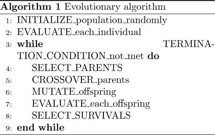
An evolutionary cycle starts with an initialization of a population of solutions, normally, represented as binary, integer, or real-valued vectors (line 1). After initialization, the evaluation of solutions is launched (line 2). Then, the while loop introduces the evolutionary cycle (lines 3–9). that is terminated with the termination condition. In each evolutionary cycle, the parent selection operator selects two parents, which contribute to mixing their genetic material with the crossover and mutation operators by creating new offspring (lines 5–6). Next, the quality of offspring is evaluated with the fitness function (line 7). Finally, the survival selection operator determines those members of the current population that will transfer their genetic material to the next generations.
Moreover, the family of EA-based approaches is large, and consists of many different approaches (Del Ser et al. 2019), among others:
-
Genetic Algorithms (GA) (Goldberg 2013),
-
Genetic Programming (GP) (Koza 1992),
-
Evolution Strategies (ES) (Rechenberg 1973),
-
Evolutionary Programming (EP) (Fogel et al. 1966),
-
Differential Evolution (DE) (Storn and Price 1997).
Although all the aforementioned algorithms follow the common principle of EAs as illustrated in Algorithm 1, they differ between each other regarding the representation of individuals. For instance, the individuals in GAs are represented as binary strings, while, in the GP, as programs in the Lisp programming language. The final state automata form a population of solutions in EP, while the real-valued vectors appear in the role of population members in ES and DE.
2.3.2 Swarm intelligence-based algorithms
The inspiration for SI-based algorithms has also been drawn from nature, precisely, from collective behavior in biological systems (Blum and Merkle 2008). For, instance, some kinds of insects (e.g., honeybees and ants) and animals (e.g., fishes and birds) live in a society, e.g., honeybee’s hives, ant colonies, schools of fish, and flocks of birds. Thus, they expose the swarm intelligence in the following sense: Although the particles (also agents) of swarms are capable of performing only simple tasks, they can deal with complex problems together as a group. In line with this, decision-making in a swarm is decentralized, while the particles are capable of self-organization. They interact between each other using some kind of communication that can be either direct or indirect (Fister et al. 2015). In the former case, information is transmitted without the intervention of the environment, while, in the latter case, individuals are not in direct contact, because the communication is conducted via environmental data.
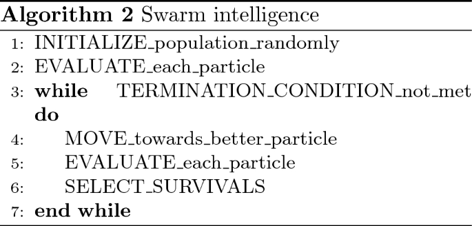
Similarly as in EAs, the SI-based algorithms also operate with a population of solutions that is called a swarm of particles in the sense of SI. The particles represent solutions of the problem to be solved, and are, typically, defined as real-valued vectors (Fister et al. 2022). During the optimization cycle, they move within the problem search space towards the better ones, and, in this way, discover new, potentially better solutions. Normally, the moves are described regarding the physical equations that mimic the moves of particles in natural biological systems. Also here, only the best particles are selected for the next generations, while the optimization cycle is terminated using a termination condition.
The pseudo-code of the SI-based algorithms is illustrated in the Algorithm 2 (Engelbrecht 2005), from which it can be seen that it differs from Algorithm 1 in line 4, where the move operator is applied in place of parent selection and variation operators as in EAs (lines 4–6).
Until the end of the last decade, a flood of newly developed SI-based algorithms emerged that raised criticism in the nature-inspired community (Sörensen 2015) about the question of how novel these algorithms were, and if they did not hide behind their famous metaphor taken from nature’s inspiration. The critics slowed down the flood, and, nowadays, only the more valuable algorithms can find a way to the research community. Although the majority of the SI-based algorithms are represented with real-valued vectors (Fister et al. 2022) and, therefore, the classification to this criteria, as by EAs, is not possible, one of the first atteempts to classify them was proposed in (Fister Jr et al. 2013). Actually, this classification was based on their inspirations from nature.
2.4 NiaPy framework
A NiaPy library (Vrbančič et al. 2018) is a framework of nature-inspired algorithms implemented in the Python programming language. This package is distributed under the MIT licence, and enables potential developers to avoid the implementation of these algorithms, which can sometimes be a difficult, complex, and tedious task. The implementations of algorithms in the library are verified, while their codes comply with the last Python standards. Currently, the library consists of 29 original nature-inspired, 7 modified, and 6 other algorithms.
Together with the aforementioned algorithms, a lot of test problems are also appended into the library. This fact enables the users to compare various algorithms between each other easily, and helps them to decide which algorithm to apply for solving their practical problems. Due to its simplicity of use, this library has also become an unavoidable tool for comparing the different nature-inspired algorithms at various universities around the world.
3 Experimental environment
In this section, we present our experimental environment, that involved a hardware unit consisting of three sensors, which allowed us to acquire data, all software and hardware components used for data collection, and the data preprocessing techniques applied to them.

Concept of the smart agriculture
The concept of the smart agriculture in our study is illustrated in Fig. 1, from which it can be seen that different IoT sensors monitor the land characteristics. Via a rural network, they are connected to a network access point, that serves for data collection and enables them access to the Internet. The collected data are reduced and preprocessed, in order to map only those indicators to extracted features that refer to soil monitoring. Obviously, each data entry is supplemented with its date and time information. Such data then enter into data analysis, in which interesting patterns (also knowledge) are mined. The decision-making process is started based on the interesting patterns. The results of this process can be represented in two ways: (1) to explain unexplained data, and (2) to propose clues for performing actions. The former serve as an input to the XAI that suggests to the farmer what to do in a specific situation, while the latter proposes an action that could be performed by the agriculture controlled system (e.g., start to irrigate a plant for 10 min). Let us notice that the study is focused only on the data collection, preprocessing, and data analysis. Due to the complexity of XAI, the last step remains a subject of the future work.
Implementing the concept of smart agriculture demands hardware and software components that must be integrated into a control system. In summary, the system in smart agriculture consist of the following components:
-
Hardware unit,
-
Data collection,
-
Data preprocessing,
-
TS-NARM with nature-inspired algorithms.
In the remainder of the paper, the aforementioned components are illustrated in detail.
3.1 Hardware unit
The hardware unit consists of sensors connected into a rural network, and an access point for acquiring data from the sensors and transmitting them to the Internet. Thus, the prototype hardware unit was built. Table 2 lists all the hardware components that were used in our solution. All the applicable sensors have been welded permanently to a simple perfboard for the sake of proof-of-concept, and wired to the ESP32 NodeMCU module. Standard communication protocols were utilized. Figure 2 visualizes a collage of the individual elements.

A sketch photo of the used elements
Actually, the ESP32 NodeMCU module represents the heart of the system and enables processing power for the data collection. The data are obtained via an Adafruit BH1750 light intensity sensor, DHT22 air temperature and humidity sensor, and Soil Moisture Hygrometer sensors. They are transferred to the webserver in predefined time periods, where these are stored in a database.
3.2 Data collection
Data from the sensors, also Sensor Data (SD), are acquired as a tuple:
where the light, temperature, humidity, and moisture indicators are obtained from the corresponding sensors.
Actually, the tuples SD are acquired in a specific time period that are defined by the user. Thus, it holds, the shorter the time period, the more detailed the acquired data. These are transmitted to the Internet server using a straightforward Python application running on the web server, pprocessing the HTTP requests utilizing a web.py library.
3.3 Data preprocessing
Data preprocessing is usually one of the most critical steps in the whole data science process. Data preprocessing can be defined as a set of methods that enhance the overall quality of the raw data and try to enrich it (Fan et al. 2021; Fister et al. 2022; Fister Jr. et al. 2022). Essentially, two tasks are required in the time series data preprocessing phase:
-
Data reduction,
-
Feature extraction.
The first preprocessing task enables grouping the data in time frames, while the second is devoted to data enrichment.
Time series TS is defined as a sequence of the collected data tuples \(SD_i\) for \(i=1,\ldots ,T\):
where T denotes the number of data tuples in time series (also time series size).
The lack of measured indicators prevents the TS-NARM to produce any specific insights. Therefore, we must enrich collected data by additional features reflecting a better outlook on time-series data. Time series Frame TF is obtained by a data reduction ML preprocessing method, where it is expected that the method analyzing TF provides the same results as analyzing the original TS. In line with this, a set of indicators collected in TS:
is reduced by a set of modifiers:
In order to determine a set of compound features, a Cartesian product of sets MODIFIER and INDICATOR is calculated except for the indicators TIME and DATE. The results of the feature extraction is illustrated in Table 3, where each compound feature is represented as a concatenation of \(MODIFIER\times INDICATOR\) denoted by a character ‘_’, while indicator DATE is mapped to the feature SEQUENCE and the indicator TIME to the feature CLASS. Thus, the modifiers are defined mathematically as follows:
where \(SD_i.INDICATOR\) for \(i=1,\ldots ,T\) specifies particular indicator collected by i-th frame of the specific TS. While the definition of the first three modifiers is self-explanatory, the modifier \(DIF\_INDICATOR\) is expressed as an difference of the indicator measured at the end and the beginning the time period and thus highlights a variance of the values within the TS. The feature SEQUENCE is calculated such that the starting date is attached to value \(SEQUENCE=0\), and then the value is incremented by one for each next date. The indicator TIME in the form hh : mm : ss is mapped firstly to a timestamp timestamp as:
and then to the proper feature CLASS according to the following equation:
where K denotes the number of time intervals, into which the 24-hour period (i.e., 86,400 sec) is divided. The selection of the proper value of K is crucial for the results of the optimization.
In summary, the time series database D of dimension \(N\times M\), where N denotes the number of transactions in the database, and M is the number of features, where each transaction is defined as a sequence of the features defined in Table 3.
3.4 Time series ARM with NI-algorithms
The purpose of this section is to present the mathematical foundations of TS-NARM and the necessary modifications that must be applied to nature-inspired algorithms for implementing TS-NARM. In our study, the following nature-inspired algorithms are applied:
-
Differential Evolution (DE) (Storn and Price 1997),
-
Genetic Algorithm (GA) (Goldberg 2013),
-
Particle Swarm Optimization (PSO) (Kennedy and Eberhart 1995),
-
Success-history based adaptive differential evolution using linear population size reduction (LSHADE) (Tanabe and Fukunaga 2014),
-
self-adaptive differential evolution (jDE) (Brest et al. 2006).
Actually, two components of nature-inspired algorithms need to be modified by implementation of the TS-NARM, i.e., representation of solutions and fitness function. Let us mention that the implementations of the original aforementioned algorithms are taken from NiaPy library.
3.5 Time series ARM
TS-NARM is a new paradigm, which treats a transaction database as a time series data. In line with this, the formal definition of the NARM problem needs to be redefined. In the TS-NARM, the association rule is defined as an implication:
where \(X(\Delta t)\subset O\), \(Y(\Delta t)\subset O\), and \(X(\Delta t)\cap Y(\Delta t)=\emptyset\). The variable \(\Delta t=[t_1,t_2]\) determines the sequence of the transactions arisen within the interval \(t_1\) and \(t_2\), where \(t_1\) denotes the start and \(t_2\) the end time of the observation. The measures of support and confidence are redefined as follows:
where \({ conf_t }(X(\Delta t) \implies Y(\Delta t))\ge C_{\max }\) and \({ supp_t }(X(\Delta t) \implies Y(\Delta t))\ge S_{\max }\) denotes the confidence and support of the association rule \(X(\Delta t)\implies Y(\Delta t)\) within the same time interval \(\Delta t\).
Let us highlight Eq. (15) with the following example: Let us assume the itemset is given as follows:
and the transaction database captures features of passed 5 days, where each day is divided into 24 classes (i.e., total 120 transactions). If 2 matches in temperatures between \(18^\circ C\) and are \(20^\circ C\) are found in 5 days within the specified time interval [12, 14], the itemset has support \(supp([12,14])=\frac{2}{5}=0.4 .\)
The other aforementioned NARM measures (i.e., inclusion and amplitude) are independent on time and, consequently, they are employed in their original form.
3.5.1 Representation of solutions
The individuals in the nature-inspired algorithms \({\textbf{x}}^{(t)}_i\) for \(i=1,\ldots ,Np\) are encoded as a real-valued vector (genotype):
where each element \(x^{(g)}_{i,j}\) for \(j=1,\ldots ,16\) determines four quadruples determining the compound features \(Feat^{(g)}_k\) for \(k=1,\ldots ,4\) into the transaction database, \(\Delta t_i\) denotes the i-th time interval, \(Cp_i\) the cutting point, and g is the generation number. Thus, each numerical feature \(\textit{Feat}^{(g)}_{\pi _j}\) consists of four real-valued elements decoded (phenotype) as:
where permutation \(\Pi =(\pi _1,\ldots ,\pi _m)\) served for modifying the position of the feature within the association rules. Technically, all first elements denoting the corresponding features are sorted in descendent order:
while their ordinal values determine their position in the permutation.
The two middle elements within quadruple encode a real-valued interval of feasible values \([lb^{(g)}_{\pi _j},ub^{(g)}_{\pi _j}]\) expressed as:
and
where \(\textit{Lb}_{\pi _j}\) and \(\textit{Ub}_{\pi _j}\) denote the lower and the upper values of the particular feature as found in the transaction database.
The threshold value denotes the presence or absence of the feature \(\textit{Feat}^{(g)}_{\pi _j}\) in the observed association rule according to the following equation:
where \(\textit{rand}(0,1)\) draws a value from uniform distribution in interval [0, 1].
The time interval \(\Delta t\) is calculated according to the following expression:
where K denotes the number of classes.
As the last element, the so-called cutting point is added to each vector that distinguishes the antecedent of the rule from the consequent ones. The cutting point Cp is expressed as:
where \({ Cp }_i\in [1,3]\).
Finally, the results of this so-called genotype-phenotype mapping, where the values encoded into genotype are decoded into phenotype, is association rule \(X\implies Y\) consisting of antecedent X and consequent Y separated by an implication sign positioned at the point determined by the variable Cp.
3.5.2 Definition of the fitness function
We tailored the fitness function presented in (Fister et al. 2018) to deal with time series data as follows:
where \(\alpha\), \(\beta\), \(\gamma\), and \(\delta\) denote weights of the support, the confidence, the inclusion, and the amplitude of the association rule \(X\Rightarrow Y\) decoded from the vector \({\textbf{x}}^{(t)}_i\).
4 Results
The goal of the experimental study was two-fold: (1) to analyse a behavior of the system in smart agriculture, and (2) to show that the nature-inspired algorithms for TS-NARM can be applied in smart agriculture. In line with this, an experimental environment was established as illustrated in the last section, which enable creating a transaction database. Then, the nature-inspired algorithms for TS-NARM were applied to searching for hidden relationships between features in the transaction database.
Two experiments were conducted in order to justify our hypotheses:
-
Analysis of a behavior of the system in smart agriculture,
-
Comparative study of five nature-inspired algorithms for TS-NARM.
In the remainder of the paper, the experimental setup is reviewed, then the algorithm configurations are discussed, and finally, the results of the aforementioned experiments are illustrated.
4.1 Experimental setup
For the purpose of our study, Aloe Vera plant served as a plant for simulation of our smart agriculture concept. As can be seen at the Fig 3, a rural network is built using sensors connected directly to the ESP32 NodeMCU control process unit. The unit is powered by a power bank of 20000 mAh capacity.

Experimental environment
Three sensors for light, air temperature and humidity, and moisture sense land characteristics and transmit sensor data in approximately 5 sec intervals. The sensor data form time series of duration 1 h. This means, that each time frame (also transactions) bears characteristics of \(12\,/\min \times 60\,\min =720\) sensor data, in other words \(T=720\).
In summary, the transaction database contains data accumulated in 14 days. Consequently, it consists of \(14\times 24=336\) different transactions.
4.2 Algorithm configurations
In our study, five nature-inspired algorithms were applied as follows: PSO, GA, jDE, DE and LSHADE. Thus, all implementations of algorithms were taken from the NiaPy library, where default parameters were taken from NiaPy examples (Vrbančič et al. 2018) (Table 4). The number of function evaluations for all algorithms was set to \(MaxFEs=50,000\) and all algorithms had the population size of 200. We performed ten independent runs for each algorithm in test.
4.3 Analysis of a behavior of the system in smart agriculture
The system presents a cost-effective solution in smart agriculture that supports: data acquiring, data collection, and data preprocessing. Therefore, the purpose of the test was to analyse how the system behaves in the sense of the following system’s performance metrics:
-
Accuracy,
-
Reliability,
-
Robustness,
-
Scalability.
The system performance metrics are defined as follows: The System Accuracy (SA) reflects a measurement accuracy of the entire system based on four components (sensors) that represent potential sources of errors. The components are listed as illustrated in Table 5.
The SA metric is calculated as follows:
where the Absolute Accuracy \(AA_i\) for \(i=1,\ldots ,4\) is expressed as \(\frac{Accuracy_i}{\Delta _i}\). Thus, the variable \(Accuracy_i\) is presented in Table 5, while the variable \(\Delta _i\) represents a measuring range.
According to (McConnell 2004), reliability is defined as ”The ability of a system to perform its requested functions under stated conditions whenever required.”. The metric is connected with Mean Time Between Failures metric, expressed as:
where the variable uptime denotes the system up-time, and the \(number\_of\_breakdowns\) refers to the number of system breakdowns. The reliability metric Rel maps the MTBF to the interval [0, 1] using the following equation:
Robustness is defined by the same author (McConnell 2004) as ”The degree to which a system continues to function in the presence of invalid inputs or stressful environmental conditions.”. The robustness metric \(R(x_i,S)\) is calculated for specific system design consisting of components \(\{x_i\}\) for \(i=1,\ldots ,n\) undergo the set of scenarios (i.e., different environmental conditions) \(S={s_1,...,s_n}\).
Scalability means the ability of the system to adjust to an increasing load. Here, we are interested in how the system accommodates greater demands by adding more hardware resources. In the lack of hardware components, no particular metric is devised for this feature in the study. However, this issue is treated in more detail in a discussion section later in the paper.
Indeed, the test comprises of evaluating three system components: hardware unit (data acquiring), data collection, and preprocessing. In line with this, the system underwent to continuous operating in duration of 14 days (Table 6). Thus, the acquired data from sensors are collected approximately each 5 seconds. In total, the system transmitted 233,980 records onto the web.
The results of data collection are depicted in Table 7, from which it can be seen time series consisting of eight sensor data records acquired in 15.9.2022 starting at 00:00:04 AM. Each record consists of indicators obtained by light, temperature, humidity, and moisture sensors. The BH1750 light sensor provides 16-bit light measurements in lux, and measures light from 0 (night) to 100K lux (day). Temperature sensor senses temperature in range \(-40^\circ C\) to \(80^\circ C\). Humidity measuring range is in interval \(0\,\%\) RH to \(100\,\%\) RH with measurement accuracy of \(\pm 2\,\%\) RH. Soil moisture is detected by a simple water sensor, while the moisture values ranging from 0 to 2300. The moisture sensor’s loose accuracy is due to the differences in wet/dry responses, namely if the sensor is dry and water level is rising, this is to be counted as a dry response. Vice versa, if water level is dropping, the sensor still remains wet to a certain degree above the water level, which lowers its accuracy. Data and time values are added by the web server.
As can be seen from Table 7, all data were obtained from measuring point number 1 during the night due to value 0 measured by light sensor. The values from other sensors remained almost constantly, while the variances of their values could be ascribed to the measurement accuracy of the particular sensor.
Due to the big number of features obtained as a result of preprocessing, the illustration of the transactions saved into transaction database is omitted in the paper. Instead of this, the statistics of the preprocessed transactions is summarized in Table 8, from which it can be seen that 336 transactions (time frames) emerged as a result of preprocessing.
4.4 Comparative study
The experiments were focused on evaluating the proposed nature-inspired algorithms for TS-NARM according to the standard ARM measures. The algorithms in the comparative study used parameter settings as illustrated in Table 4. The results of the experiments are illustrated in Table 9 depicting the achieved values according to four measures (i.e., support, confidence, inclusion, and amplitude), and average lengths of corresponding antecedent and consequent per each observed algorithm. Columns ’Numrules’ and ’Intervals’ are added to the table and denote the number of mined rules and the percentage of intervals covered by the rule, respectively.
Interestingly, the best results according to support and confidence are distinguished by the DE, while the best results according to inclusion are achieved by the jDE, and according to amplitude by the PSO. The longer length of features in antecedent and consequent are mined by the jDE and PSO, respectively, where the length of both measures overcome the value of 3 attributes per antecedent/consequent. The maximum number of rules were mined by the PSO (i.e., 11, 911), while the minimum by the GA (only 205). As a matter of fact, all algorithms excellent cover the intervals in the rules.
The results are compared also using Wicoxon 2-paired non-parametric statistical tests with confidence level \(\alpha =0.01\). Thus, each classifier was composed by the results according to the fitness value, support and confidence ARM measures obtained for each algorithm in 10 runs. As a result, the classifier of size 30 was obtained (i.e., \(10\times 3=30\)) that enters into the Wilcoxon tests. Moreover, to the results of these tests also metric mined rules per second is calculated as the ratio of the average run time in seconds and the average number of mined rules.
The results of the comparative study, where the best results are bold, are illustrated in Table 10, from this, the results of the 2-paired tests are presented as a matrix of algorithms entered into the Wilcoxon tests. When the results of the two algorithms are significantly different (i.e., \(p<0.01\)), the corresponding pair is denoted with the symbol 3’\(\checkmark\)’ in the matrix. The symbol ’\(\infty\)’ denotes that the same algorithm cannot be entered into the test.
The Wilcoxon tests revealed that the results of the GA are significantly different (i.e., worse) from the results of all the other algorithms in the study. Interestingly, the other algorithms did not differ significantly, except the results of the original DE are significantly worse than the results of the jDE.
According to the average run time, the results showed that the lSHADE was the most expensive. On the other hand, this algorithm, together with the PSO, outperforms the results of the other algorithms according to the average number of mined association rules per second because both algorithms mined more than eight association rules per second.
4.5 Time complexity
A time complexity analysis of the nature-inspired algorithms is a challenging task because they are too general, while the analysis is focused on the specific optimization algorithm by solving the specific problem. The nature-inspired algorithms can be adapted to solve more problems easily without expert knowledge of the problem’s domain. On the other hand, the problem-specific algorithms run correctly (i.e., they can find the optimal solution in each run) and efficiently (i.e., less time complexity) by solving the specific problem.
When the nature-inspired algorithms are analyzed from the algorithm’s theory, we are interested in identifying the upper bound of their time complexity and their lower bound of solution quality. Indeed, they are stochastic according to their nature, and consequently, they are analyzed as randomized algorithms in computer science. Typically, these are analyzed using (Jansen 2015):
-
Approaches based on the Markov chain,
-
Schema theorem,
-
Run-time analysis.
The run-time analysis adopts the nature-inspired algorithms from two perspectives: (1) an algorithm’s correctness and (2) an average-case behavior. The average-case behavior is strongly connected with the termination condition of the specific nature-inspired algorithm. Our study considers the maximum number of fitness function evaluations, while its correct value is determined using the convergence graph analysis.
5 Discussion, conclusions and further research
The following conclusions can be obtained according to the results of the first test: The result \(SA=0.2062\) reveals that the system accuracy is around \(\pm 20\,\%\). However, the moisture sensor presents the weakest part of the system, while its accuracy is reported as \(\le 20\,\%\), which is typical for this kind of sensor. Although the applied sensor is low-cost, the acquired data are accurate, mainly because errors can be compensated by averaging values of the considerable number of measurements. In general, the conducted test showed that the system is fully reliable that is shown calculating the metrics \(MTBF=\frac{14\cdot 24\cdot 60}{1}=20,160\) and \(Rel=\frac{20,160}{20,160}=1\). This means the system operated continuously over the observed 14 days without system breakdown. It underwent different weather conditions (e.g., stormy, rainy, sunny, etc.) and more day-night cycles during this period. In each of these scenarios, the system acquires data typically and accurately. This fact justifies the robustness of the system. Finally, the system is scalable as well because the ESP32 sensors can be organized into independent modules (elements), which severely boosts its scalability. For instance, such independent modules can be planted in intervals across fields to cover large agricultural areas. Standard communication protocols, such as GPRS, ethernet, or wifi, dependent on the area’s scale, can be utilized to ensure the convergence of diversified data into a central database.
The following conclusions may summarize the results of the second test carried out: The DE is excellent in searching for rules, where there exist good relationships between features regarding either other feature or the total number of transactions, respectively. The best use of the number of features in antecedent and consequent is identified by the GA, while the best covering of the numeric intervals is achieved by the PSO. On the other hand, the GA discovered the less number of association rules comparing with the other algorithm in test. Indeed, the highest number of rules is mined by the PSO. Consequently, the higher the number of mined rules, the better support and confidence, and contrary, the smaller the number of mined rules, the richer the association rules in the sense of the number of features in antecedent and consequent.
However, there are also several bottlenecks that were found when running experiments. All blockages are summarized as follows:
-
Some intervals are occasionally omitted, and after the run, there are no rules linked to a specific interval.
-
Sometimes algorithms identify a rule with very high fitness, consequently, the algorithm falls within the local optimum, and after that, it is tough to find good rules in the other intervals.
-
After the initial experiments, we found that it is essentially to ensure more evaluations since they ensure that we find rules in different intervals.
In the future, it would be necessary to find a better local search or switch between different intervals to capture as much association rules as possible. It is recommended that a new metric being added to the fitness function, which would also control how much of the intervals are covered in the final results. Finally, we will explore extending/enhancing our work by incorporating high utility with frequent pattern mining (Fournier-Viger et al. 2016), Fournier-Viger et al. (2020) to get more relevant rules for use in the real world.
Code and data availability
The datasets and source codes are available from the corresponding author on reasonable request.
References
Agrawal R, Srikant R, et al. (1994) Fast algorithms for mining association rules. In: Proc. 20th int. conf. very large data bases, VLDB, volume 1215, pp 487–499. Citeseer
Agrawal H, Dhall R, Iyer KSS, Chetlapalli V (2020) An improved energy efficient system for iot enabled precision agriculture. J Ambient Intell Humaniz Comput 11(6):2337–2348
Alejandro Barredo A, Díaz-Rodríguez N, Del Ser J, Bennetot A, Tabik S, Barbado A, García S, Gil-López S, Molina D, Benjamins R et al (2020) Explainable artificial intelligence (xai): concepts, taxonomies, opportunities and challenges toward responsible ai. Inform Fusion 58:82–115
Bajželj B, Richards KS, Allwood JM, Smith P, Dennis JS, Curmi E, Gilligan Christopher A (2014) Importance of food-demand management for climate mitigation. Nat Clim Chang 4(10):924–929
Blum C, Merkle D (2008) Swarm intelligence: introduction and applications. Natural computing series. Springer Science and Business Media
Brest J, Greiner S, Bošković B, Mernik M, Žumer Viljem (2006) Self-adapting control parameters in differential evolution: a comparative study on numerical benchmark problems. IEEE Trans Evol Comput 10(6):646–657
Dabre Kanchan R, Lopes Hezal R, D’monte Silviya S (2018) Intelligent decision support system for smart agriculture. In: 2018 International Conference on Smart City and Emerging Technology (ICSCET), pp 1–6. IEEE
Del Ser J, Osaba E, Molina D, Yang X-S, Salcedo-Sanz S, Camacho D, Das S, Suganthan PN, Coello CAC, Herrera F (2019) Bio-inspired computation: where we stand and what’s next. Swarm Evol Comput 48:220–250
Eiben AE, Smith James E (2015) Introduction to evolutionary computing, 2nd edn. Springer Publishing Company, Incorporated (ISBN 3642436013)
Engelbrecht AP (2005) Fundamentals of computational swarm intelligence. Wiley
Fan C, Chen M, Wang X, Wang J, Huang B (2021) A review on data preprocessing techniques toward efficient and reliable knowledge discovery from building operational data. Front Energy Res. https://doi.org/10.3389/fenrg.2021.652801
FAO, Rome, Italy (2009) The state of food and agriculture. http://www.fao.org/3/a-i0680e.pdf, Accessed: 05 Nov 2022
FAO, Rome, Italy (2017) Soil organic carbon: the hidden potential. http://www.fao.org/3/a-i6937e.pdf. Accessed: 2022 Nov 05
Fister I, Iglesias A, Galvez A, Ser del J, Osaba E (2018) Differential evolution for association rule mining using categorical and numerical attributes. In: International conference on intelligent data engineering and automated learning, pp 79–88. Springer
Fister I Jr, Yang X-S, Fister I, Brest J, Fister D (2013) A brief review of nature-inspired algorithms for optimization. Electrotech Rev 80(3):116–122
Fister I Jr, Podgorelec V, Fister I (2021) Improved nature-inspired algorithms for numeric association rule mining. In: Vasant P, Zelinka I, Weber G-W (eds) Intelligent computing and optimization. Springer International Publishing, Cham, pp 187–195
Fister Jr I, Fister I, Salcedo-Sanz S (2022) Time series numerical association rule mining for assisting smart agriculture. In: 2022 International Conference on Electrical, Computer and Energy Technologies (ICECET), pp 1–6. IEEE
Fister D, Fister I Jr, Karakatic S (2022) Dynfs: dynamic genotype cutting feature selection algorithm. J Ambient Intell Humaniz Comput. https://doi.org/10.1007/s12652-022-03872-3
Fogel LJ, Owens AJ, Walsh MJ (1966) Artificial intelligence through simulated evolution. Wiley
Fournier-Viger P, Chun-Wei LJ, Dinh T, Le HB (2016) Mining correlated high-utility itemsets using the bond measure. In: Hybrid Artificial Intelligent Systems: 11th International Conference, HAIS 2016, Seville, Spain, April 18-20, 2016, Proceedings 11, pp 53–65. Springer
Fournier-Viger P, Zhang Y, Lin Jerry C-W, Dinh D-T, Bac Le H (2020) Mining correlated high-utility itemsets using various measures. Logic J IGPL 28(1):19–32
Goldberg DE (2013) Genetic algorithms. Pearson Education
Hahsler M, Hornik K (2007) New probabilistic interest measures for association rules. Intell Data Anal 11(5):437–455
Issad HA, Aoudjit R, Rodrigues JJPC (2019) A comprehensive review of data mining techniques in smart agriculture. Eng Agric Environ Food 12(4):511–525
Iztok F, Damjan S, Xin-She Y, Iztok F Jr. (2015) Adaptation and hybridization in nature-inspired algorithms. Adaptation and hybridization in computational intelligence. Springer, pp 3–50
Jansen T (2015) Analyzing evolutionary algorithms. Springer Publishing Company, Incorporated
Kennedy J, Eberhart R (1995) Particle swarm optimization. In: Proceedings of ICNN’95 - International Conference on Neural Networks, 4:1942–1948
Koza JR (1992) Genetic programming: on the programming of computers by means of natural selection. MIT press
Lucio C, Danilo C, Carmelo A, Giuseppe D, Annamaria C, Maristella M, Raj K, Dimitrios M, Kun-Mean H, François P, Jean-Pierre C, Gao H, Hongling S (2020) Introduction to agricultural iot. In: Castrignanò A, Buttafuoco G, Khosla R, Mouazen AM, Moshou D, Naud O (eds) Agricultural internet of things and decision support for precision smart farming. Academic Press, pp 1–33
McConnell S (2004) Code complete, 2nd edn. Microsoft Press (ISBN 0735619670)
Mishra M, Choudhury P, Pati B (2021) Modified ride-nn optimizer for the iot based plant disease detection. J Ambient Intell Humaniz Comput 12(1):691–703
Mohapatra H, Rath AK (2022) Ioe based framework for smart agriculture. J Ambient Intell Humaniz Comput 13(1):407–424
Ouafiq EM, Saadane R, Chehri A (2022) Data management and integration of low power consumption embedded devices iot for transforming smart agriculture into actionable knowledge. Agriculture 12(3):329
Rechenberg I (1973) Evolutionsstrategie Optimierung technischer Systeme nach Prinzipien der biologishen Evolution. Optimierung technischer Syste Frommann-Holzboog, Stuttgart
Sahitya G, Balaji N, Naidu CD (2016) Wireless sensor network for smart agriculture. In: 2016 2nd International Conference on Applied and Theoretical Computing and Communication Technology (iCATccT), pp 488–493. IEEE
Sörensen K (2015) Metaheuristics-the metaphor exposed. Int Trans Oper Res 22(1):3–18
Storn R, Price K (1997) Differential evolution-a simple and efficient heuristic for global optimization over continuous spaces. J Global Optim 11(4):341–359
Tanabe R, Fukunaga AS (2014) Improving the search performance of SHADE using linear population size reduction. In: Proceedings of the 2014 IEEE Congress on Evolutionary Computation, CEC 2014, pp 1658–1665
Torres-Tello J, Seok-Bum K (2021) Interpretability of artificial intelligence models that use data fusion to predict yield in aeroponics. J Ambient Intell Humaniz Comput. https://doi.org/10.1007/s12652-021-03470-9
Tzanetos A, Dounias G (2021) Nature inspired optimization algorithms or simply variations of metaheuristics? Artif Intell Rev 54(3):1841–1862
Vrbančič G, Brezočnik L, Mlakar U, Fister D, Fister I (2018) Niapy: python microframework for building nature-inspired algorithms. J Open Source Softw 3(23):613
Funding
This work was supported by the Slovenian Research Agency (Research Core Funding Nos. P2-0057, P5-0027). This work has also been partially supportted through project PID2020-115454GB-C21 of the Spanish Ministry of Science and Innovation (MICINN).
Author information
Authors and Affiliations
Corresponding authors
Ethics declarations
Conflict of interest
The authors declare that they have no potential conflict of interest.
Additional information
Publisher's Note
Springer Nature remains neutral with regard to jurisdictional claims in published maps and institutional affiliations.
Rights and permissions
Open Access This article is licensed under a Creative Commons Attribution 4.0 International License, which permits use, sharing, adaptation, distribution and reproduction in any medium or format, as long as you give appropriate credit to the original author(s) and the source, provide a link to the Creative Commons licence, and indicate if changes were made. The images or other third party material in this article are included in the article's Creative Commons licence, unless indicated otherwise in a credit line to the material. If material is not included in the article's Creative Commons licence and your intended use is not permitted by statutory regulation or exceeds the permitted use, you will need to obtain permission directly from the copyright holder. To view a copy of this licence, visit http://creativecommons.org/licenses/by/4.0/.
About this article

Cite this article
Fister, I., Fister, D., Fister, I. et al. Time series numerical association rule mining variants in smart agriculture. J Ambient Intell Human Comput 14, 16853–16866 (2023). https://doi.org/10.1007/s12652-023-04694-7
Received:
Accepted:
Published:
Issue Date:
DOI: https://doi.org/10.1007/s12652-023-04694-7