Abstract
Advanced validation of cluster analysis is expected to increase confidence and allow reliable implementations. In this work, we describe and test CluReAL, an algorithm for refining clustering irrespective of the method used in the first place. Moreover, we present ideograms that enable summarizing and properly interpreting problem spaces that have been clustered. The presented techniques are built on absolute cluster validity indices. Experiments cover a wide variety of scenarios and six of the most popular clustering techniques. Results show the potential of CluReAL for enhancing clustering and the suitability of ideograms to understand the context of the data through the lens of the cluster analysis. Refinement and interpretability are both crucial to reduce failure and increase performance control and operational awareness in unsupervised analysis.
1 Introduction
Clustering is a method for discovering data groups (or clusters) based on the location and density of data points in the space drawn by point features. In addition to other mathematical tools, clustering is used to obtain descriptions of data and discover patterns hidden inside. It becomes particularly useful in multi-dimensional, large datasets that are difficult to analyze by means of traditional methods and are commonly deemed as chaotic, messy, and challenging.
However, clustering algorithms are habitually very sensitive, non-robust, and biased by their own algorithmic approach and hyperparameters. Thus, clustering often “explains” data with forced structures that do not match the analyzed data. Main reasons behind unsatisfactory clustering are:
-
The algorithm fails because it lacks capabilities or due to a wrong parameterization.
-
The data do not match structures that are explainable with clustering.
Regardless of the reason that caused the failure, we need to know whether the clustering output is misleading; otherwise, the purpose of the analysis will be affected. Therefore, we need to assess how reliable and representative clustering results are. Internal validity algorithms cope with this task by ranking solutions with metrics that are commonly based on cluster separation and compactness. However, they have some downsides, one of which is being relative in nature; that is, they are useful for establishing comparisons and discrimination between various solutions, but rarely for evaluating them alone. Except for extreme cases, validity algorithms do not state if a solution space is suitable or not, but only what is the best solution space in a comparison. Note that they could all be wrong and not be noticed by the analyst (or the system in which clustering is embedded).
We previously addressed this problem and consequently proposed a set of indices to validate clustered spaces in an absolute manner [20]. On the basis of this work, we here developed ideograms to represent clustered data in a compact way and an algorithm to improve clustering regardless of the chosen technique. Ideograms are useful as keys for the human analyst to interpret and understand datasets, but also as codes to support automated decision making in systems that incorporate clustering for explaining data contexts.
Internal validity indices often apply assumptions and suffer from limitations, namely: globularity (aimed clusters are assumed globular); subjectivity (different clustering solutions can be equally valid); uncertainty (the best cluster-representation might be unreachable); suboptimality (suboptimal solutions are acceptable); unsolvability (data might not fit cluster structures). Further discussion on these aspects can be found at [20]. Here, we briefly discuss globularity, since at least this constraint is common and extensible to most clustering validity approaches.
The methods presented in this paper are suitable for multi-dimensional spaces in which globular clusters (or globular approximations) are expected. Therefore, our methods (alike most cluster validity methods) are not useful for applications like spatial clustering, in which accurately capturing cluster shapes plays a determining role. Methods typically applied in such scenarios are density-based techniques that require special validation measures [10, 31]. A second exception is subspace clustering [25]. In subspace clustering, clusters are searched in lower dimensions, meaning that in the original space clusters might be hyperplanes or lines in hyperplanes, again requiring specialized validity methods for their evaluation.
Note that complex shapes have a strong connection with visual information and maps, but not necessarily with data. For instance, the difference between an “S”-shaped cluster in a five-dimensional space when compared with the same cluster taken as globular might be irrelevant or arbitrary for the application purpose. Our proposal subscribes this principle for many real-life applications, in particular when the suboptimality assumption also applies.
This paper is an extension of a conference contribution [21]. This extended version presents the enhanced implementation of CluReAL.v2. In addition to changes in the algorithm core, CluReAL.v2 uses fast kernel density estimations, graph-based rules to fuse sub-clusters (or micro-clusters), and a deeper definition of cluster kinship relationships. Additionally, it solves multimodal clusters, which previously remained untreated. Evaluation experiments are much more demanding now, since we compare CluReAL.v2 with other clustering optimization techniques based on random parameter search and parameter sweeps. Additional algorithms and datasets are used (including high-dimensional and other popular ones taken from the related literature for clustering evaluation). Evaluations are now conducted with external validation metrics that use ground-truth labels. Finally, critical difference diagrams are also used to show if performance differences among tested methods are statistically significant.
In the following sections, we give a short summary of internal cluster validation methods and the theoretical background of our approach (Sect. 2) and we explain CluReAL for clustering refinement (Sect. 3) and SK ideograms for interpreting clustered data (Sect. 4). We evaluate our proposals with experiments that are described in Sect. 5. Results are shown and discussed in Sect. 6. The work closes with the conclusions in Sect. 7. Additionally, Appendix shows CluReAL configurations to cope with high overlap and comparisons between CluReAL.v1 and CluReAL.v2.
2 Clustering validation
Clustering validation (a.k.a. cluster validity or internal validation) consists in the evaluation of clustering only using topological or geometrical characteristics of the data. In other words, there is no ground-truth partition to compare with. Several studies provided comprehensive comparisons of different cluster validity indices [2, 44], to cite some of the most popular: Silhouette [37], Calinski–Harabasz [7], or the Davies–Bouldin index [11].
2.1 GOI: Absolute internal validation
Validity indices are often based on different ways of evaluating cluster separation and compactness. Note that, if it is possible to assume that the algorithm worked properly, validity indices would be giving information about how compliant the input space is to cluster-like structures. This concept is the basis of the GOI validation [20], which proposed two types of indices: individual overlap indices for each cluster (oi) and global overlap indices for the joined solution (G), and two modalities: strict and relaxed.
The mathematical formulations of oi indices are:
where \(\Gamma _{Aj}\) is the cluster inter-distance (centroid-to-centroid) between clusters A and j. \(\Lambda _{\text {cor,A}}\) is the radius of the core volume of cluster A, which is defined as the median intra-distance of cluster A (datapoints in A to the centroid \(c_A\)). \(\Lambda _{\text {ext},A}\) is the radius of the extended volume of cluster A, which is defined as the mean plus two times the standard deviation of intra-distances in cluster A. This follows Chebyshev’s inequality, which ensures that the extended radius covers at least 75% of datapoints regardless of the underlying distribution [39].
Therefore, oi indices measure cluster separation and compactness after representing each cluster as a pair of concentric hyperspheres, in which the inner one assumes homogeneous cores by using robust statistics and the outer one uses Chebyshev’s inequality to force external layers to adapt to any possible point distribution. Such approach provides a simplified model of the space that can be treated mathematically (Fig. 1).

\(\Lambda \), \(\Gamma \), and oi allow modeling the clustered space as hyperspheres. For easy viewing, only magnitudes for calculating \(G_{str}\) are shown. In the example, negative \(oi_{str,1}\) and \(oi_{str,2}\) capture the overlap between Cluster 1 and Cluster 2
Finally, G indices can be defined for estimating separation and compactness in the whole dataset. Given a dataset with k clusters, a G function takes the form:
From here, we can derive either a strict index or a relaxed index for the whole dataset depending on the radii (\(\Lambda \)) and oi indices used, specifically:
Additionally, a minimum G index is defined to satisfy applications in which any cluster overlap is deemed as highly undesirable:
Together, \(G_{\text {str}}\), \(G_{\text {rex}}\), and \(G_{\text {min}}\) are capable of describing and evaluating the clustered space in an absolute manner. In [20], the keys to interpret G indices and a methodology to apply them for improving the quality of clustering are given. We build the methods presented here on such knowledge, oi and G indices becoming the backbone of the algorithm outlined in Sect. 3 and the ideograms described in Sect. 4.
2.2 External validation
Since traditional validation is based on cluster compactness and separation estimations, it might show limitations in certain scenarios [26]. When the ground truth is available, the validation techniques used are called external validation (or just evaluation). These methods measure the match between the found classification and the ideal partition given by the ground truth. Among the most popular, we find: the Jaccard index [22], the Rand index [34], or the mutual information score [41]. Since we have the ground-truth available in our experiments (and also to improve the contrast with the optimization methods under test, which use internal validation), we use external methods in the final evaluation.
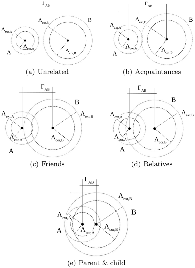
Types of cluster kinship for two random clusters A and B. Symbols are described in Sect. 3.1
3 CluReAL
General-purpose methods to improve or refine clustering are scarce. Precedents commonly focus on the establishment of best parameters, particularly the number of clusters [30, 48], either they are designed for specific algorithms [6], or devise ways to make the manual correction easier [18].
In this work, we design and develop CluReAL (from Clustering Refinement ALgorithm), a general-purpose tool to refine clustering regardless of the algorithm used. The rationale behind CluReAL is modeling discovered clusters with \(\Lambda \) and \(\Gamma \) radii hyperspheres, later merging, splitting, or dismantling them based on oi distances, relative densities, and the detection of multiple point cores in singular clusters. Ultimately, CluReAL aims to improve G indices. An early prototype of CluReAL(.v1) was introduced in [21]. Here, we describe the current, enhanced version of the algorithm (CluReAL.v2), which considerably differs from the previous version in that parameterization has been simplified, graphs are used to connect clusters, a deeper kinship definition is used, and automatic resolution of multimodal clusters is incorporated. Both versions are compared in Section A.2.
3.1 Algorithm Description
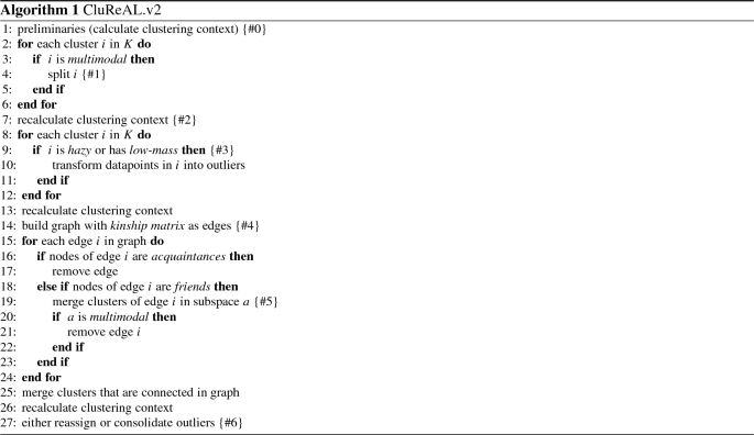
The pseudocode of CluReAL.v2 is shown in Algorithm 1. We comment on relevant aspects:
-
#0
Preliminaries. CluReAL operates with some values obtained from the clustering. These are context variables:
-
(a)
The number of clusters (k), with K being the set of clusters.
-
(b)
Cluster cardinality (mass or number of elements). |A| for cluster A.
-
(c)
Cluster centroids. \(c_A\) for cluster A.
-
(d)
Cluster inter-distance. Given clusters A and B with centroids \(c_A\) and \(c_B\), respectively, and d as the Euclidean distance, the cluster inter-distance between A and B can be defined as:
$$\begin{aligned} \Gamma _{AB} = d(c_A,c_B). \end{aligned}$$(7) -
(e)
Cluster core and extended radii. Given cluster A with datapoints \(A=\{x_0,x_1,...,x_N\}\) and centroid \(c_A\), the set of intra-distances is:
$$\begin{aligned} D_A = \Big \{d(x_0,c_A),d(x_1,c_A),...,d(x_N,c_A)\Big \}. \end{aligned}$$(8)The core radius is defined as the median intra-distance:
$$\begin{aligned} \Lambda _{\text {cor},A}=Q_{0.5}(D_A) \end{aligned}$$(9)with \(Q_{0.5}\) being the quantile function with \(p=0.5\), ergo the Median. The extended radius is established as:
$$\begin{aligned} \Lambda _{\text {ext},A} = \mu _{_{D_A}} + 2\sigma _{_{D_A}} \end{aligned}$$(10)with \(\mu \) and \(\sigma \) being the mean and standard deviation of cluster A intra-distances, respectively.
-
(f)
Cluster density. CluReAL uses cluster densities that are relative to the density of the whole dataset taken as a single cluster O. Therefore, the relative density of a cluster A is:
$$\begin{aligned} \rho _A= \frac{\frac{|A|}{\Lambda _{\text {cor},A}} - \frac{|O|}{\Lambda _{\text {ext},O}}}{\frac{|O|}{\Lambda _{\text {ext},O}}}. \end{aligned}$$(11) -
(g)
Cluster kinship. Extended and core radii and cluster inter-distances are used to define types of cluster kinship. They are described in the set of equations 12. Figure 2 shows graphical diagrams to better understand kinship relationships.
$$\begin{aligned} \begin{aligned} {unrelated } \quad&\Gamma _{AB}> ( \Lambda _{\text {ext},A} + \Lambda _{\text {ext},B})\\ {acquaintances } \quad&\Gamma _{AB} \le ( \Lambda _{\text {ext},A} + \Lambda _{\text {ext},B}) \;\; \wedge \\ \quad&\Gamma _{AB}> ( \Lambda _{\text {cor},A} + \Lambda _{\text {cor},B}) \\ {friends } \quad&\Gamma _{AB} \le ( \Lambda _{\text {cor},A} + \Lambda _{\text {cor},B}) \;\; \wedge \\ \ \quad&\Gamma _{AB}> \text {max}(\Lambda _{\text {ext},A}, \Lambda _{\text {ext},B}) \\ {relatives } \quad&\Gamma _{AB} \le \text {max}(\Lambda _{\text {ext},A}, \Lambda _{\text {ext},B}) \;\; \wedge \\&\Gamma _{AB} > \text {min}(\Lambda _{\text {ext},A}, \Lambda _{\text {ext},B}) \\ {parent-child } \quad&\Gamma _{AB} \le \text {min}(\Lambda _{\text {ext},A}, \Lambda _{\text {ext},B}).\\ \end{aligned} \end{aligned}$$(12) -
(h)
Cluster multimodality. A multimodal cluster is any cluster that shows more than one peak of point concentration. To establish whether cluster A is multimodal, CluReAL searches for peaks in one-dimensional kernel density estimations (KDE) of cluster features separately [42]. If any feature shows more than one peak, cluster A is labeled as “multimodal”. There are diverse methods to implement very fast KDE [35]. By default, CluReAL.v2 opts for a convolution FFT-based computation with the Silverman’s rule of thumb for the bandwidth calculation [43].
-
(a)
-
#1
Solving multimodal clusters. In contrast to CluReAL.v1, CluReAL.v2 solves multimodal clusters by analyzing them separately as isolated subspaces. By default, the algorithm used for splitting multimodal clusters is a k-means variation [40]. A cluster detected as multimodal may not be finally split if it conflicts with subsequent fusing rules (e.g., multimodal clusters show close kinship).
-
#2
Recalculating the clustering context. Each time that the clustering structure is modified, recalculating clustering context variables (inter-distances, intra-distances, densities, radii, masses, etc.) is required to fit the new solution.
-
#3
Removing superfluous clusters. CluReAL transforms hazy clusters and low-mass clusters into outliers. The qualities of being hazy and low-mass are controlled by the external hyperparameters MRD (minimum relative density) and MCR (minimum cardinality ratio), respectively. CluReAL admits configurations in which defining outliers is not allowed and all points must be assigned to clusters (see point #6).
-
#4
Connecting clusters with graphs. After removing low-density and low-mass clusters, a graph is built in which nodes represent clusters and edges are kinship relationships. Edges among acquaintances are cut, and edges between friends are also cut if the cluster resulting from merging such nodes forms a multimodal cluster; otherwise, edges among friends are kept (Fig. 3). Such rules for cutting edges become automatically more radical (i.e., the tolerated kinship levels are reduced) whenever only one cluster is detected in the solution. The level of severity of these rules can also be controlled by an external, optional parameter (Section A.1).
-
#5
Merging clusters. Clusters that are connected by graph edges are merged together.
-
#6
Reassigning or consolidating outliers. Regardless of the fact that we consider outliers as noise, extreme values, or isolated points between clusters, labeling data points as outliers is an application design option. CluReAL.v2 uses a hyperparameter called OS (outlier sensitivity) to establish how far from centroids outliers discovered by the initial algorithm or by the CluReAL refinement can remain. OS is a coefficient that divides \(\Lambda _{\text {cor}}\). High OS values allow more outliers, whereas \(\hbox {OS}=0\) reassigns all potential outliers to clusters. The reassignment uses the closest centroid for setting the final label.

Example of CluReAL graph before processing. Nodes represent clusters, and edge widths correspond to kinship relationships. Nodes that are not connected are unrelated. The thinnest edges (acquaintances and friends) are likely to be cut, and the nodes that remain will be merged. This example shows a clustering that does require refinement, namely: either the original clustering was conducted with a too-high k, or a considerable number of multimodal clusters were detected
3.2 Parameterization
CluReAL.v2 uses three main hyperparameters: MCR, MRD, and OS. They are intuitive and can be left with default values for most scenarios, since they concern to the minimum mass of clusters (relative to the total mass), minimum density (relative to the overall density), and sensitivity to outliers (relative to sizes of the cluster cores modeled with robust statistics).
The subjectivity and suboptimality assumptions introduced in Sect. 1 make the use of hyperparameters and thresholds unavoidable. As a general rule, clustering cannot escape from certain ambiguity, therefore being impossible to clearly determine a best solution in certain situations (Figure 4 shows some examples).
3.3 Complexity
As defined in Algorithm 1, CluReAL.v2 is a straightforward, low-complex procedure. The main bottleneck appears in the KDE used for calculating multimodality. Considering that from the three variable magnitudes—n: number of data points, m: number of dimensions, and k: number of clusters—the critical factor is n, fast solutions (as the FFT-based one used in CluReAL.v2) show \(O(n \log n)\) time complexity [35]. Note that CluReAL calculates density estimations in a one-dimensional fashion, this being extremely faster than KDE in multi-dimensional spaces.
CluReAL.v2 incorporates k-means to solve multimodal clusters by default. K-means methods are habitually variations of the Lloyd’s algorithm [27], whose time complexity is considered linear [3]. If CluReAL is adjusted to use a different algorithm for solving multimodality, complexity should be accordingly recalculated, but note that multimodal clusters are expected to take a small fraction of the whole mass in normal cases.
4 Context interpretation based on clusters
Interpreting clustering is required in all applications, and key when clustering is used as a tool to provide information about the data context. Note that this is a problem different to dimensionality reduction, visualization of high-dimensional spaces, or clustering spaces that have been previously reduced. Here, the cluster analysis already summarized data and the challenge is properly interpreting clustering outputs in connection with input data altogether.
Dendrograms [9, 32] and Silhouette plots [37] are traditionally the most common methods to visualize clustering results. Another popular approach is leveraging the high-interpretability of decision trees and using them for extracting rules from clustering outcomes [4]. Among other transformation techniques, multi-dimensional scaling (MDS), principal component analysis (PCA), and self-organizing maps (SOM) have been proposed for projecting the clustering solution into two dimensions while respecting as much as possible topologies and distances [46].
These options are still complicated to interpret, might be incomplete, require the careful attention of an expert, and hardly offer a quick impression of the context. Additionally, they are not easily translatable for a machine decision-making process. More complete reads of the context are possible by using several clustering outputs such as the number of clusters, inter-distances, intra-distances, masses, and densities. An example is the 3D mountain visualization implemented in CLUTO [24], which also uses MDS for locating centroids. Here, clusters are represented with Gaussian curves, the shape being a rough estimate of the data distribution within clusters. The peak height reflects the cluster internal similarity, the volume represents the mass, and colors are proportional to cluster-internal deviations (red for low, blue for high).
4.1 SK Ideograms
Based on the GOI indices and other measures introduced in Sects. 2 and 3, we developed a set of symbols that can be combined to form ideograms. Such ideograms offer an interpretation of the dataset context from the perspective of the cluster analysis. Figure 5 shows some examples to understand all possible ideograms. Some of the symbols can be combined together, while others exclude each other. Henceforth, we refer to them as SK ideograms (from symbolic keys).
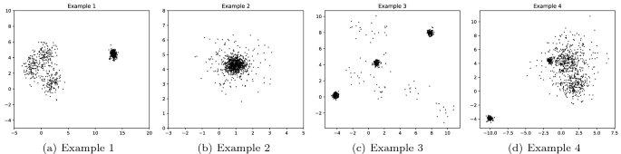
Examples of ambiguity in clustering. How many clusters are shown in Example 1? Two clusters with different densities or four clusters, three of them strongly overlapped? Should external data points in Example 2 be considered outliers and how many of them? Do data points in low density areas in Example 3 form clusters? Should they be considered outliers/noise instead? How many clusters does the space in Example 4 show?
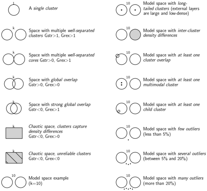
Models for SK ideograms
4.2 Example of clustering interpretation
Figure 6a shows an example of a small dataset with three dimensions. The cluster analysis correctly found five clusters. The remaining plots are different ways of visualizing clustering results. (Note that we usually cope with multi-dimensional spaces that have more than three dimensions, fact that makes the direct visual examinations much harder.)
The dendrogram (Fig. 6b) does not find an optimal partition, but bisects data based on similarity criteria. Branch height marks the similarity between the clusters below (alike clusters will have similar branch heights). Only by checking a dendrogram, it is not possible to unequivocally assess if cluster overlap happens, if some points were erroneously clustered, or simply the quality of the clustering from a general perspective.
The Silhouette plot (Fig. 6c) shows the Silhouette index of every single datapoint, which will be close to 1 when maximum compactness/separation is achieved. The plot places the “green” cluster as the best one (far, dense) and the “blue” cluster as the worst one (close to others, low density). Silhouette indices are easy to interpret when they take extreme values, but confusing for intermediate cases. For instance, we cannot discern if the “blue” cluster is legitimate or if, instead, it is an arbitrary merger of some subclusters. Figure 6d shows a two-dimensional projection of the original space by using MDS. Only cluster centroids are projected, surrounded by circles that represent average and maximum intra-distances. Although helpful, such projections can lead to wrong impressions of cluster volumes and inter-distances. In the example, the MDS projection suggests a cluster overlap that does not actually happen in the original problem space.
The mountain visualization in Fig. 6e adds some extra information to the MDS case that is useful; however, it may raise misleading interpretations about the cluster quality and actual overlap. Unlike the previous options, the SK ideogram is a simple symbol focused on interpreting the quality of the clustering from a cluster compactness–separation perspective. Note that, in the example (Fig. 6f), it is the only representation that clearly summarizes the problem as “a space with five well-separated clusters with inter-cluster density differences.” Compared to the other options, the SK ideogram is not only a visualization, but also intrinsically incorporates the interpretation and evaluation of the clustered space. As such, it is useful for the data scientist, but can also be easily shared and integrated into stand-alone machine learning frameworks.
5 Evaluation experiments
We conducted evaluation experiments by comparing the effect of CluReAL refining a wrong parameterized clustering against a traditional clustering optimization performed by selecting the best clustering among a set of candidates that used different parameterizations. Figure 7 displays the experimental setup scheme with a block diagram. Experiments are organized in two sets:
-
Two-dimensional data. We use 12 different datasets for these experiments and one clustering algorithm (a k-means variant, introduced in Sect. 5.2). In addition to showing final scores, we plot the clustered spaces for both competing methods. We also show SK ideograms. These two-dimensional examples are provided to enable the reader to visually understand and further assess CluReAL refinements and SK interpretations, which would be hardly feasible in spaces with more dimensions.
-
Multi-dimensional data. Here, we test CluReAL with 134 multi-dimensional synthetic datasets designed according to seven possible characteristics intrinsic to the input space. We use six different underlying clustering algorithms (Sect. 5.2).
All experiments in addition to examples, codes, extended results, method implementations, and other material are available for reuse and replication in our GitHub repository.Footnote 1 Ground-truth labels for all datasets used are also available.

Example of clustering visualizations. a Original 3D dataset already clustered (colors correspond to categories). b A dendrogram shows datapoint IDs in the x-axis and associates them with tree branches. c In the Silhouette plot, the x-axis is scores and the y-axis is datapoint IDs. d “MDS” stands for the multidimensional scaling of centroids, in which circles show average and maximum intra-distances. e The visualization used in CLUTO [24] represents clusters as Gaussian-shaped 3D mountains. f SK ideogram. It summarizes clustered data as five well-separated clusters different densities
5.1 Datasets
Most of the datasets used in the experiments were generated with the MDCGen tool [19], which has been particularly designed for testing clustering. Note that Arbelaitz et al. [2] have proven that there is not a significant difference between synthetic and real datasets when using them for evaluating cluster validity algorithms. Datasets are divided into the following groups:
-
Separated clusters datasets consist of spaces between 2 and 23 dimensions, with a number of clusters between 3 and 7, and 5000 data points without outliers. Clusters are multivariateFootnote 2 Gaussian shape and designed to show high inter-distances. There are 20 datasets for the multi-dimensional tests and one dataset for the two-dimensional tests.
-
Close clusters datasets use the same configuration as separated clusters datasets, but the number of clusters is between 10 and 14, showing low inter-distances. Again, there are 20 datasets for the multi-dimensional tests and one dataset for the two-dimensional tests.
-
Density-differences datasets show the same basic configuration as separated clusters datasets, but the underlying distributions are tuned in both multivariate and radial ways. Moreover, distributions are set at random among the following: uniform, Gaussian, logistic, triangular, gamma, and ring-shaped clusters. There are 20 datasets for the multi-dimensional tests and one dataset for the two-dimensional tests. Note that in all groups density differences occur due to the different cluster cardinalities, but in this specific one they are forced to be more extreme by varying point generation distributions.
-
Low-noise datasets have the same configuration as separated clusters datasets, but add between 5% and 15% outliers. There are 20 datasets for the multi-dimensional tests and one dataset for the two-dimensional tests.
-
High-noise datasets have the same configuration as separated clusters datasets, but add between 15% and 40% outliers. There are 20 datasets for the multi-dimensional tests and one dataset for the two-dimensional tests.
-
Complex datasets have the same configuration as density-differences datasets, but add between 5% and 15% outliers. There are 20 datasets for the multi-dimensional tests and one dataset for the two-dimensional tests.
-
High-dimensional datasets have been proposed for checking clustering algorithms in high-dimensional spaces by Fränti et al. [17]. All datasets have nine clusters, but different numbers of datapoints. In our experiments, we use ten datasets with dimensions equal to 2, 3, 5, 10, 15, 32, 64, 256, 512, and 1024.
-
Popular two-dimensional datasets are taken from previous publications related to clustering evaluation, namely: A-sets [23], S-sets [16], and the unbalance dataset [36].
-
Real datasets with labels for evaluating clustering are very scarce in the literature. Instead, real labeled data are commonly oriented to supervised classification, in which labels are not necessarily bound to the internal geometry of the feature space, but to their utility within the application. In other words, classes need not be linked to groups, or not cleanly. To include also real data in our experiments, we have used four popular datasets that are addressed for multi-class classification, namely: Breast Cancer, Diabetes, Digits, and Wine datasetsFootnote 3. To enhance class separation, we have transformed original spaces by using t-SNE, which is prone to create representations with cluster-like structures [28].
5.2 Algorithms and benchmark
We used six popular clustering algorithms. They can be divided into two groups:Footnote 4
-
1.
Algorithms that require an initial number of clusters as input:
-
2.
Density-based algorithms:
Any clustering algorithm must be adjusted in order to achieve meaningful results. The main hyperparameter to set in Group 1 is the expected number of clusters (k). HDBSCAN and OPTICS (Group 2) are hierarchical versions of the original DBSCAN [15]; as such, a hyperparameter with a strong effect in both is minPts. This parameter defines how many neighbors a point must have to be considered a core point, i.e., part of the cluster bulk. HDBSCAN does not perform clustering, but produces a hierarchy of density estimates. The final definition of clusters in the HDBSCAN implementation used in our experiments applies flat cluster extraction on top of the discovered hierarchy [8, 29]. In addition to the minimum cluster size, for the cluster extraction a eps hyperparameter is necessary to establish cluster separation, ultimately affecting granularity (either a few big clusters, or many smaller clusters). Instead, OPTICS requires a hyperparameter called xi, which determines the minimum steepness in a reachability distance to fix cluster boundaries.
In our experiments, we compare CluReAL refining a suboptimal clustering with default or arbitrary parameters against the best clustering found by traditional methods for clustering optimization. The competitor method is established according to the algorithm group:
-
Silhouette k-sweep (Group 1). For every dataset, each algorithm is run ten times with different k-values. We use the ground truth to establish sweep values around the ideal and ensure that this optimization method reaches an optimal solution. The performance that obtains the best overall Silhouette score [37] is saved to be compared with CluReAL refinement. Instead, CluReAL refines a deliberately wrong clustering with a k considerable higher than the provided by the ground truth (\(k_{CRAL}=k_{GT}+10\)).
-
Random parameter search (Group 2). Here, for each dataset algorithms are run 20 times with different hyperparameter combinations obtained by random search. minPts and eps are set with values around adjustment recommendations given by [38] and [33]. xi in OPTICS is searched between 0.05 and 0.2. In both algorithms, the minimal cluster size is always fixed at 5% of the total number of data points. Instead, CluReAL refines the clustering found with fixed values of \(minPts=5\), \(xi=0.08\) for all cases, a minimal cluster size of 5%, and the knee value suggested by Rahmah and Sitanggang [33] for each dataset.
5.3 Evaluation metrics
Although clustering optimization methods apply internal validity measures for their adjustment, we use the adjusted mutual information (AMI) score to evaluate the matching between the ground truth and the final clustering given by the competing options. AMI is the adjusted version of the Mutual Information score (MI) to account for chance [45]. The adjusted version compensates for the fact that MI is usually higher when comparing solutions with larger number of clusters, irrespective of whether or not they share more information. Thus, AMI obtains a better fit of the score range [0, 1] (“1” standing for a perfect matching). AMI has been found a suitable “general-purpose” measure for clustering validation and algorithm comparison and design.
6 Results
6.1 Two-Dimensional experiments
Figure 8 shows final clusterings for the two-dimensional datasets. Every subfigure is formed by four plots: (1) The top-left plot shows the best k-means clustering obtained with the Silhouette k-sweep; (2) the top-right plot shows the suboptimal clustering after CluReAL refinement; and (3) and (4) bottom plots show the respective SK ideograms for the clustering above. AMI scores are shown in Table 1. We comment on them case by case.
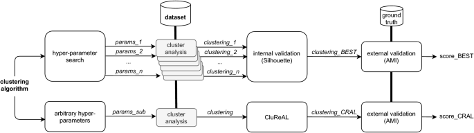
Scheme of evaluation experiments

Scatter plots showing clustered solutions of the two-dimensional tests. Clustered data points are drawn with different colors, black being for outliers. SK diagrams are displayed below the scatter plots

-
Separated clusters (Fig. 8a). This scenario consists of seven well-separated clusters with different masses, but the same underlying Gaussian distribution. Both optimization methods find perfect solutions due to the relative simplicity of the scenario. SK ideograms are identical, showing seven well-separated clusters. Also note that SK finds inter-cluster density differences, long-tailed clusters, and multimodal clusters, properties that are difficult to check visually due to the image resolution. Density differences are marked because clusters with different masses occupy similar areas (the most-dense and less-dense clusters have 591 and 91 data points, respectively). Wrong warnings about multimodality are sometimes triggered by low-density clusters that do not have enough points to show a clear, compacted core.
-
Close clusters (Fig. 8b). This dataset shows 11 clusters very close to each other, some of them overlapping and some of them with low density. This type of scenarios is considerably challenging for clustering. The best solution from the k-sweep merges some clusters that overlap, discovering nine clusters; additionally, it also assigns some data points to the wrong neighbor cluster. CluReAL refinement obtains a significantly better solution, but it is not able to separate the two clusters that show the strongest overlap. On the other hand, SK ideograms slightly differ, not only in the number of clusters, also in the global separation of clusters, which is higher for the CluReAL case. In both ideograms, the small circle on the top-left part of the figure marks that a strong overlap has been detected even in spite of the fact that clusters do not overlap in general.
-
Clusters with density differences (Fig. 8c). The dataset shows different distributions generating three clusters with varied shapes and sizes. This challenge was correctly solved by both competing options. SK ideograms are consistent with the clustered data. They show three long-tailed, well-separated clusters with different densities.
-
Dataset with low noise (Fig. 8d). This dataset is formed by five Gaussian clusters surrounded by about 10% outliers. This example shows how even low noise affects normal clustering. The best k-sweep solution is distorted by noise and merges the central clusters. By refining a suboptimal k-means, CluReAL correctly discloses the five clusters and removes most noise data points. The SK ideogram detects the central multimodal cluster in the k-sweep solution and the overlap in spite of general separated clusters in both cases.
-
Dataset with high noise (Fig. 8e). This dataset is formed by six Gaussian clusters surrounded by about 30% outliers. The higher the noise, the more distorted traditional clustering become. Here, the best k-sweep solution is considerably misleading as it merges four clusters and forms a fifth cluster out of noise. The refined CluReAL labeling discloses the six expected clusters and identifies most outliers. Note how SK symbols inform about the strong general overlap and multimodality in the best k-sweep clustering due to the heterogeneity of the found clusters and their big size with coinciding boundaries.
-
Complex dataset (Fig. 8f). This dataset is formed by seven clusters and combines previous data peculiarities: noise, different shapes, masses and densities, close and separated clusters, and overlap. Scenarios like this one are extremely challenging for clustering algorithms. The best k-sweep solution establishes two clusters that perform a very rough summary of the problem. On the other hand, CluReAL refinement is able to disclose the main shapes and filter intermediate noise, even in spite of the fact that two clusters are still merged with their closest neighbors. SK symbols should warn about multimodality in the best k-sweep case, but it fails due to the specific placement of clusters, which dodge the feature-by-feature multimodality detection. This issue is prone to be less likely the more dimensions the dataset has.
-
S-datasets (Fig. 8g–i). These datasets are formed by 15 Gaussian clusters with 5000 data points and different degrees of cluster overlap. S1 is satisfactorily solved by both competitors. In S2, clusters show more overlap; k-sweep obtains a good performance, while CluReAL starts finding problems to properly separate clusters and tends to merge them. Note how the SK ideogram for CluReAL in S2 reduces the number of clusters to 14, but still informs about the existence of multimodal clusters that CluReAL was not able to split. The overlap is even stronger in S3 and CluReAL wrongly merges overlapped clusters. The SK ideogram is consistent with the clustered context and explains it as chaotic, where clustering is merely capturing density differences. k-means sweep is significantly better in S3, even in spite of creating an additional cluster from arbitrary splits (green cluster on the bottom-right part of the top-left plot in Fig. 8i). CluReAL has two alternatives to properly deal with high overlap:Footnote 5 (a) by modifying edge-pruning rules during the refinement or (b) by using data coresets. Both options are described in Section A.1.
-
A-datasets (Fig. 8j–k). These datasets are formed by Gaussian clusters of 150 data points that are close to each other and even show some overlap, A2 with 35 clusters and A3 with 50 clusters. The refinement of CluReAL on suboptimal solutions shows slightly better performances than the best k-sweep options in both cases. Clusters are better formed, and local minima problems are minimized. As for the SK representations, note that, since all clusters have the same size and cardinality, there are no density differences among them.
-
Unbalance dataset (Fig. 8l). This last dataset is extremely complicated for any algorithm due to the strong differences in size and density. There are eight clusters, five of them with 100 data points each and the remaining three with 2000 data points each. Moreover, the clusters with lower cardinality occupy larger areas. CluReAL refining suboptimal k-means overcomes the difficulties, whereas the best k-sweep fails to correctly split the problem space and merges two times two low-density clusters. Note that the SK ideogram notices it by marking multimodality.
6.2 Multi-Dimensional experiments

Boxplots of AMI scores over all 134 multi-dimensional datasets together
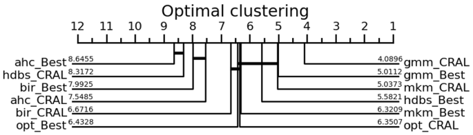
The critical difference diagram compares methods with Wilcoxon signed-rank tests [14]. The best methods are placed on the right side. Methods that do not show a significant difference are connected with thick lines
Table 3 summarizes AMI scores per dataset group. Additionally, Fig. 9 shows boxplots with all scores together, each boxplot corresponding to a different algorithm and a different optimization method. A critical difference diagram comparing all combinations is also provided in Fig. 10. Both the boxplot and the critical difference diagram are calculated over the introduced 134 different datasets and, together with Table 3, show equivalent results, namely a general tendency of CluReAL refinement on suboptimal clustering to equal or outperform traditional optimization by hyperparameter search and internal validation. This is best seen in Table 2, which shows the rank obtained by each method in the overall comparison and, additionally, if there is a statistically significant difference in results obtained from Sweep vs CRAL optimizations when checked alone for every tested algorithm. We take a closer look at Table 3 results from two perspectives:
-
Type of data challenge. The type of data challenge does not considerably affect the performance of CluReAL refinement when compared to traditional optimization. It is specially pertinent for cases in which outliers are present and the algorithm used is not specifically prepared to deal with them (low-outlier and high-outlier datasets). Datasets that show a higher performance variability and differences between competing options are the ones included in the density differences and complex groups, but the suitability of CluReAL is more related to the algorithm used than the type of data challenge. Tests also show that CluReAL is able to refine clustering even in high-dimensional spaces.
-
Clustering algorithm to refine. Experiments show that CluReAL refinement tends to outperform searching for the optimal k with k-sweeps regardless of the algorithm used. The improvement is particularly outstanding for Gaussian mixture models clustering (gmm). Algorithms in Group 2 show a different behavior. The overall performance of CluReAL compared with random hyperparameter search is only slightly better in the case of OPTICS (opt) and clearly worse for HDBSCAN (hdbs). It is important to remember that CluReAL does not carry out clustering per se, but works on a previously obtained solution, tolerating a certain degree of error in the original clustering. Unlike the case of k for Group 1 (which depends on the number of actual clusters), hyperparameters searched in Group 2 tests depend on data dimensionality and point separation. Hence, performance scores when using suboptimal parameters are prone to be more extreme in Group 2 than in Group 1. In other words, in Group 1 we can expect some correlation between the performance score and the selected k (the closer to the ideal value the better); instead, in Group 2 a non-perfect parameterization will likely generate either a good clustering or a very distorted clustering. In the first case, CluReAL is not necessary; in the second case, the refining process can hardly take advantage of the previous solution. This explains the performances of CluReAL in the HDBSCAN and OPTIC cases. The arbitrary parameterization in HDBSCAN tends to generate very poor clustering; instead, it commonly generates good clustering in OPTICS. Finally, the critical diagram in Fig. 10 and Table 2 confirms the CluReAL refinement performed statistically better than hyperparameter search for agglomerative hierarchical clustering (ahc), Birch (bir), Gaussian mixture models (gmm), and minibatch K-means (mkm), equivalent for OPTICS (opt), and worse for HDBSCAN (hdbs). It also suggests that refining Gaussian mixture models clustering with CluReAL is the most recommended option when highly accurate clustering is desired and clear insight for parameterization is not available.
6.3 Final remarks
Note that the importance of refinement may not be reflected if only the improvement in AMI scores is taken into account. This is due to the strong inertia generated by correctly classified points. Results in close, A2, and A3 two-dimensional experiments clearly illustrate this issue. Despite CluReAL only obtaining a slight improvement in AMI scores, its clustering has better quality: It is less prone to local minima errors and avoids sectioning clusters in an incoherent way.
Moreover, the convenience of simply refining one clustering (CluReAL) over selecting the best of a set (parameter search or sweep) becomes evident in cases where clustering is embedded in a framework or as the size of the data starts increasing. In such cases, parameter search might soon become unfeasible. This is clearly shown in the example of Fig. 11. The figure shows time performances of the studied clustering optimization combinations in a sensitivity analysis in which the parameter under test is the number of data points: 500, 1000, 2500, 5000, 10000, 25000. The scenario contains 30 isotropic Gaussian clustersFootnote 6 of five dimensions. Sweep-based optimization (“Best”) uses 20 different configurations.

Time performances of the clustering optimization methods in response to variations in the number of data points. In spite of the overlap, values of all CRAL curves are significantly lower than the best curves as the number of data points increases

Example of adjusting CluReAL to cope with overlap (S2 dataset). From left to right: a ground truth; b CluReAL, default configuration; c CluReAL, increased pruning; d CluReAL, using coresets; (e) CluReAL, increased pruning and using coresets

Example of adjusting CluReAL to cope with overlap (S3 dataset). From left to right: a ground truth; b CluReAL, default configuration; c CluReAL, increased pruning; d CluReAL, using coresets; e CluReAL, increased pruning and using coresets
7 Conclusions
In this work, we have presented CluReAL, an algorithm for improving clustering regardless of the used clustering technique given some fundamental assumptions. Based on the same principles, we have also introduced SK ideograms, symbolic representations that enable fast, intuitive, automated interpretations of clustered spaces.
Experimental tests with six different algorithms have shown how, as a general rule, CluReAL refining a wrongly parameterized clustering outperforms the best clustering obtained from random hyperparameter search, with special prominence given to the combination of CluReAL and Gaussian mixture models. The more than one hundred datasets used were designed to match common situations and challenges in unsupervised setups: separated clusters, close clusters, low level of outliers, high level of outliers, clusters that show density differences, complex scenarios that combine all previous characteristics, high-dimensional spaces, and some popular datasets previously proposed for algorithm evaluation.
Outcomes of clustering are prone to be misleading and are traditionally difficult to validate and interpret. Enhancing cluster refinement and interpretability is strongly required to increase the reliability of automated systems and clustering-based artificial intelligence.
Notes
In multivariate clusters, distributions for the point-value generation are applied independently for each feature. In radial clusters, point values are generated ensuring that their distance to the centroid follows the selected distribution.
Minibatch K-means, agglomerative hierarchical clustering, Gaussian mixture models, Birch, and OPTICS in our experiments are Python implementations from Scikit-learn v0.22, https://scikit-learn.org/stable/index.html. HDBSCAN v0.8.18 is from https://HDBSCAN.readthedocs.io/en/latest/index.html.
Here, none of these options have been applied in order to maintain equality in the comparisons.
References
Ankerst, M., Breunig, M., Kriegel, H.P., Sander, J.: Optics: Ordering points to identify the clustering structure. SIGMOD Rec. 28(2), 49–60 (1999)
Arbelaitz, O., Gurrutxaga, I., Muguerza, J., Pérez, J.M., Perona, I.: An extensive comparative study of cluster validity indices. Pattern Recogn. 46(1), 243–256 (2013)
Arthur, D., Vassilvitskii, S.: How slow is the k-means method? In: Proceedings of the Twenty-Second Annual Symposium on Computational Geometry, Association for Computing Machinery, New York, NY, USA, SCG ’06, pp 144–153, 10.1145/1137856.1137880 (2006)
Basak, J., Krishnapuram, R.: Interpretable hierarchical clustering by constructing an unsupervised decision tree. IEEE Trans. Knowl. Data Eng. 17(1), 121–132 (2005)
Biernacki, C., Celeux, G., Govaert, G.: Assessing a mixture model for clustering with the integrated completed likelihood. IEEE Trans. Pattern Anal. Mach. Intell. 22(7), 719–725 (2000)
Bouchachia, A., Pedrycz, W.: Enhancement of fuzzy clustering by mechanisms of partial supervision. Fuzzy Sets Syst. 157(13), 1733–1759 (2006)
Caliński, T., Harabasz, J.: A dendrite method for cluster analysis. Commun. Stat. 3(1), 1–27 (1974)
Campello, R.J., Moulavi, D., Zimek, A., Sander, J.: A framework for semi-supervised and unsupervised optimal extraction of clusters from hierarchies. Data Mining Knowl. Discovery 27(3), 344–371 (2013)
Campello, R.J.G.B., Moulavi, D., Zimek, A., Sander, J.: Hierarchical density estimates for data clustering, visualization and outlier detection. TKDD 10(1), 1–51 (2015)
Campello, R.J.G.B., Kröger, P., Sander, J., Zimek, A.: Density-based clustering. Wiley Interdiscip Rev Data Min Knowl Discov 10(2), 10.1002/widm.1343 (2020)
Davies, D.L., Bouldin, D.W.: A cluster separation measure. IEEE Trans. Pattern Anal. Mach. Intell. PAMI 1(2), 224–227 (1979)
Day, W.H.E., Edelsbrunner, H.: Efficient algorithms for agglomerative hierarchical clustering methods. J. Classif. 1(1), 7–24 (1984)
Dempster, A.P., Laird, N.M., Rubin, D.B.: Maximum likelihood from incomplete data via the em algorithm. J. Royal Stat. Soc.: Ser. B (Methodol.) 39(1), 1–22 (1977)
Demšar, J.: Statistical comparisons of classifiers over multiple data sets. J. Mach. Learn. Res. 7, 1–30 (2006)
Ester, M., Kriegel, H.P., Sander, J., Xu, X.: A density-based algorithm for discovering clusters in large spatial databases with noise. In: Proceedings of the Second International Conference on Knowledge Discovery and Data Mining, AAAI Press, KDD’96, p 226–231 (1996)
Fränti, P., Virmajoki, O.: Iterative shrinking method for clustering problems. Pattern Recogn. 39(5), 761–765 (2006). https://doi.org/10.1016/j.patcog.2005.09.012
Fränti, P., Virmajoki, O., Hautamäki, V.: Fast agglomerative clustering using a k-nearest neighbor graph. IEEE Trans. Pattern Anal. Mach. Intell. 28(11), 1875–1881 (2006)
Heine, C., Scheuermann, G.: Manual clustering refinement using interaction with blobs. In: Proceedings of the 9th Joint Eurographics / IEEE VGTC Conference on Visualization, Eurographics Association, Goslar, DEU, EUROVIS-07, p 59–66 (2007)
Iglesias, F., Zseby, T., Ferreira, D., Zimek, A.: Mdcgen: Multidimensional dataset generator for clustering. J. Classif. 36, 599–618 (2019)
Iglesias, F., Zseby, T., Zimek, A.: Absolute cluster validity. IEEE Trans. Pattern Anal. Mach. Intell. 42(9), 2096–2112 (2020a)
Iglesias, F., Zseby, T., Zimek, A.: Interpretability and refinement of clustering. In: 2020 IEEE 7th International Conference on Data Science and Advanced Analytics (DSAA), pp 21–29, 10.1109/DSAA49011.2020.00014 (2020b)
Jaccard, P.: The distribution of the flora in the alpine zone 1. New Phytol. 11(2), 37–50 (1912)
Kärkkäinen, I., Fränti, P.: Dynamic local search algorithm for the clustering problem. Tech. Rep. A-2002-6, Department of Computer Science, University of Joensuu, Joensuu, Finland (2002)
Karypis, G.: Cluto-a clustering toolkit. Tech. rep., Minnesota Univ. Minneapolis Dept. of Computer Science (2002)
Kriegel, H., Kröger, P., Zimek, A.: Clustering high-dimensional data: A survey on subspace clustering, pattern-based clustering, and correlation clustering. TKDD 3(1), 1–58 (2009)
Liu, Y., Li, Z., Xiong, H., Gao, X., Wu, J., Wu, S.: Understanding and enhancement of internal clustering validation measures. IEEE Trans. Cybern. 43(3), 982–994 (2013)
Lloyd, S.: Least squares quantization in pcm. IEEE Trans. Inf. Theory 28(2), 129–137 (1982)
van der Maaten, L., Hinton, G.: Visualizing data using t-sne. Journal of Machine Learning Research 9(86):2579–2605, http://jmlr.org/papers/v9/vandermaaten08a.html (2008)
McInnes, L., Healy, J., Astels, S.: hdbscan: Hierarchical density based clustering. Journal of Open Source Software 2(11): 205 (2017)
Mirkin, B.: Choosing the number of clusters. WIREs Data Mining Knowl. Discovery 1(3), 252–260 (2011)
Moulavi, D., Jaskowiak, P.A., Campello R.J.G.B., Zimek, A., Sander, J.: Density-based clustering validation. In: SDM, SIAM, pp 839–847 (2014)
Murtagh, F.: Counting dendrograms: A survey. Discrete Appl. Math. 7(2), 191–199 (1984)
Rahmah, N., Sitanggang, I.S.: Determination of optimal epsilon (eps) value on DBSCAN algorithm to clustering data on peatland hotspots in sumatra. IOP Conference Series: Earth and Environmental Science 31, 012012 (2016). https://doi.org/10.1088/1755-1315/31/1/012012
Rand, W.: Objective criteria for the evaluation of clustering methods. J. Am. Stat. Assoc. 66(336), 846–850 (1971)
Raykar, V.C., Duraiswami, R., Zhao, L.H.: Fast computation of kernel estimators. J. Comput. Graphical Stat. 19(1), 205–220 (2010)
Rezaei, M., Fränti, P.: Set-matching methods for external cluster validity. IEEE Trans. Knowl. Data Eng. 28(8), 2173–2186 (2016)
Rousseeuw, P.J.: Silhouettes: A graphical aid to the interpretation and validation of cluster analysis. J. Comput. Appl. Math. 20, 53–65 (1987)
Sander, J., Ester, M., Kriegel, H.P., Xu, X.: Density-based clustering in spatial databases: The algorithm gdbscan and its applications. Data Mining Knowl. Discovery 2(2), 169–194 (1998)
Saw, J.G., Yang, M.C.K., Mo, T.C.: Chebyshev inequality with estimated mean and variance. Am. Stat. 38(2), 130–132 (1984)
Sculley, D.: Web-scale k-means clustering. In: Proceedings of the 19th International Conference on World Wide Web, ACM, New York, NY, USA, WWW ’10, pp 1177–1178 (2010)
Shannon, C.E.: A mathematical theory of communication. ACM SIGMOBILE Mobile Comput. Commun. Rev. 5(1), 3–55 (2001)
Silverman, B.W.: Using kernel density estimates to investigate multimodality. J. R. Stat. Soc.: Ser. B 43(1), 97–99 (1981)
Silverman, B.W.: Density Estimation for Statistics and Data Analysis. Chapman & Hall, London (1986)
Vendramin, L., Campello, R.J.G.B., Hruschka, E.R.: Relative clustering validity criteria: A comparative overview. Stat. Anal. Data Mining 3(4), 209–235 (2010)
Vinh, N.X., Epps, J., Bailey, J.: Information theoretic measures for clusterings comparison: Variants, properties, normalization and correction for chance. J. Mach. Learn. Res. 11, 2837–2854 (2010)
Doğan, Yunus, Dalkılıç, Feriştah, Birant, Derya, Kut, Recep Alp, Yılmaz, Reyat: Novel two-dimensional visualization approaches for multivariate centroids of clustering algorithms. Sci. Program. 2018, 23 (2018)
Zhang, T., Ramakrishnan, R., Livny, M.: Birch: An efficient data clustering method for very large databases. SIGMOD Rec. 25(2), 103–114 (1996). https://doi.org/10.1145/235968.233324
Ünlü, R., Xanthopoulos, P.: Estimating the number of clusters in a dataset via consensus clustering. Expert Syst. Appl. 125, 33–39 (2019)
Funding
Open access funding provided by TU Wien (TUW).
Author information
Authors and Affiliations
Corresponding author
Ethics declarations
Conflict of interest
On behalf of all authors, the corresponding author states that there is no conflict of interest.
Additional information
Publisher's Note
Springer Nature remains neutral with regard to jurisdictional claims in published maps and institutional affiliations.
This work was partly supported by the project MALware cOmmunication in cRitical Infrastructures (MALORI), funded by the Austrian security research programme KIRAS of the Federal Ministry for Agriculture, Regions and Tourism (BMLRT) under grant no. 873511.
A Appendix
A Appendix
1.1 A.1 Coping with High Overlap
CluReAL.v2 has two basic configuration options to deal with datasets that show strong overlapped:
-
1.
Stiffing edge-pruning rules. In this case, rules for cutting edges between clusters during refinement are shifted one kinship level. This implies that edges between friend clusters are always removed and relative clusters are only conditionally merged.
-
2.
Using coresets. This option assumes that cluster densities are not homogeneous. By using coresets, a significant part of the data is removed from the analysis, aiming to mainly retain cluster cores. After the refinement, cluster labels are extended to excluded data points according to distances to cluster centroids.
Figures 12 and 13 show S2 and S3 examples when CluReAL is applied with and without the previous two configuration options. In both examples, CluReAL refined minibatch K-means clustering that was set with a wrong initial \(k=25\). In both cases, adjusting parameters to deal with overlap significantly improved clustering, but when the overlap is severe and cluster densities tend to be uniform (like in S3), obtaining ideal performances by refining wrong clustering can be hardly feasible. Note that the last right plot in Fig. 13, which is when coresets and more rigid edge-pruning is applied, in spite of the fact that the SK symbol is almost equivalent to the SK symbol of the ground truth, two legitimate clusters still remain fused and an arbitrary cluster has been created instead (the pink cluster on the bottom-right corner).
1.2 A.2 CluReAL.v2 vs CluReAL.v1
Although grounded in the same ideas (i.e., G and oi indices and representations, multimodality estimations, and kinship relationships), CluReAL.v2 differs significantly from CluReAL.v1 in many aspects. The base algorithm has been modified to operate much faster and to avoid iterations; required parameters have been either simplified or made more robust; the kinship definition is more detailed and connected to a new graph representation that ultimately establishes the remaining cluster structure; finally, multimodal clusters, which were untreated before, are tackled now. In short, whereas CluReAL.v1 was devised to just enhance clustering, CluReAL.v2 has been designed as a clustering optimization alternative that can replace parameter search, which is commonly too costly for real applications.
The progress from CluReAL.v1 to CluReAL.v2 becomes obvious when their performances are compared. In Table 4, we show results after clustering a randomly selected dataset from each group of the multi-dimensional experiments. The base clustering uses a minibatch K-means with a deliberately suboptimal parameterization, and this is later refined with both CluReAL.v1 and CluReAL.v2, respectively. The advantages of CluReAL.v2 over CluReAL.v1 are clear in terms of accuracy and time performances.
Rights and permissions
Open Access This article is licensed under a Creative Commons Attribution 4.0 International License, which permits use, sharing, adaptation, distribution and reproduction in any medium or format, as long as you give appropriate credit to the original author(s) and the source, provide a link to the Creative Commons licence, and indicate if changes were made. The images or other third party material in this article are included in the article’s Creative Commons licence, unless indicated otherwise in a credit line to the material. If material is not included in the article’s Creative Commons licence and your intended use is not permitted by statutory regulation or exceeds the permitted use, you will need to obtain permission directly from the copyright holder. To view a copy of this licence, visit http://creativecommons.org/licenses/by/4.0/.
About this article

Cite this article
Iglesias, F., Zseby, T. & Zimek, A. Clustering refinement. Int J Data Sci Anal 12, 333–353 (2021). https://doi.org/10.1007/s41060-021-00275-z
Received:
Accepted:
Published:
Issue Date:
DOI: https://doi.org/10.1007/s41060-021-00275-z