Abstract
Optimal control for infectious diseases has received increasing attention over the past few decades. In general, a combination of cost state variables and control effort have been applied as cost indices. Many important results have been reported. Nevertheless, it seems that the interpretation of the optimal control law for an epidemic system has received less attention. In this paper, we have applied Pontryagin’s maximum principle to develop an optimal control law to minimize the number of infected individuals and the vaccination rate. We have adopted the compartmental model SIR to test our technique. We have shown that the proposed control law can give some insights to develop a control strategy in a model-free scenario. Numerical examples show a reduction of 50% in the number of infected individuals when compared with constant vaccination. There is not always a prior knowledge of the number of susceptible, infected, and recovered individuals required to formulate and solve the optimal control problem. In a model-free scenario, a strategy based on the analytic function is proposed, where prior knowledge of the scenario is not necessary. This insight can also be useful after the development of a vaccine to COVID-19, since it shows that a fast and general cover of vaccine worldwide can minimize the number of infected, and consequently the number of deaths. The considered approach is capable of eradicating the disease faster than a constant vaccination control method.
Introduction
Mathematical models of infectious diseases have been extensively studied over the past decades [1,2,3,4,5,6,7,8,9,10,11]. The outbreak of infectious disease has caused mortality of millions of people as well as represents a noteworthy risk to public health and may cause heavy economic and social losses [12]. Needless to say, the quick spread of the coronavirus in 2020 throughout the world is a clear evidence of the importance of research on this topic [13, 14]. Among the several models of infectious diseases, the SIR (susceptible, infected, recovered) model, introduced in [15], is probably the most studied. In spite of the fact that, it appears to be basic, the SIR model has been explored in numerous viewpoints, for example, nonlinear examination of wave going of SIR pandemic model [16], effects of discretization schemes [17, 18], HIV on small scale population [19] variable population [20, 21], and optimal control [22,23,24,25,26,27] to cite a few examples.
The SIR model has been important to clarify several key issues. One of them is the fact that there is a threshold for the strength of disease spread, wherein there is an endemic behaviour of an infectious disease. Besides that this threshold can be changed by means of vaccination [28]. More specifically, by vaccinating a sufficient percentage of the population, the disease can be eradicated. In fact, many works have addressed with some success this issue using a constant vaccination rate [3, 29, 30]. In fact, in several public health practices, a constant value of vaccination rate is adopted as target during several public campaigns [31]. Recently, the author of [32] has applied optimization techniques to find suitable vaccination strategies in an age structured SIR model.
Due to economic pressure over the government agencies all around the world, suitable vaccination campaigns are difficult to implement [33]. This fact has made several researchers turn their attention to the optimal control problem [34]. The author of [22] has considered various deterministic optimal control models for SIR-epidemics. The author has used vaccination, quarantine, screening or health promotion campaigns as forms of control. In [35] the authors have applied an optimal control strategy during flu season, the SIR model was also used in that work.
In [36], the goal was to figure ideal vaccination designs for a quickly spreading disease in an urbanized profoundly mobile population, using different types of structured SIR models. In [37] the authors have developed a time-delay SIR model to consider that infected individuals can remain sick for a period of time defined over an interval with a lower bound. An optimal impulse control strategy has been employed, the cost function considered was composed by a cost associated with the state variables and a cost associated with the vaccination (that depends on the control effort and also on delayed states). In [12] the stability and the optimal control problem for the SIR model has been investigated. The objective functional to be minimized depends on the number of susceptible and infected individuals in addition to the control effort. The authors in [38] have considered the optimal control problem for the standard SIR model, the main target was the minimization of the infection eradication time. The authors of [26] present an optimal control approach for the SIR model based on a cost index that depends on the state variables, on the control effort that is weighted by a nonlinear function and it also depends on mixed terms (product between number of infected individuals and control effort). Optimal control has also been considered to deal with the SIR model under the assumption of imprecise parameters described as intervals [39]. In that case a linear cost function of infected individuals and control effort has been employed. One may cite also the work proposed in [40] that deals with the optimal control problem for spatiotemporal SIR models. The system was described by a set of partial differential equations and the considered control variable was the spatial and temporal distribution of the vaccine.
In the aforementioned articles there are important results for the research on epidemiology. Nevertheless, the interpretation of an optimal control law for an epidemic system has been little investigated. This seems an issue that has not received attention in the literature. In this paper, we have applied optimal control to eradicate infectious diseases described by SIR models. We also exploit the optimal control law to provide qualitative insights for control policies of vaccination. Using Pontryagin’s maximum principle [34] an optimal control law that minimizes the number of infected individuals and the vaccination rate has been obtained. However, there is not always a prior knowledge of the number of susceptible, infected, and recovered individuals required to formulate and solve the optimal control problem. In a model-free scenario, a strategy based on the analytic function is proposed, where prior knowledge of the scenario is not necessary. We have noticed that a very high level of vaccination rate in the beginning of control policy, with a systematic reduction in its level can be a general principle to be used. This principle is derived from the optimal control law. The considered approach is capable of eradicating the disease faster than a constant vaccination control method. The control employed in this paper can give some insights about how to act to eradicate infectious diseases in real life. Nowadays, the unique method to eradicate or mitigate the COVID-19 is the physical distancing measurements [11, 41]. After a development of a vaccine, there is no guarantee of worldwide cover due to economical and cultural restrictions [42]. Thus, it is still important to address such a problem for the COVID-19 pandemic. The results found here can be useful to stress the importance of a global and a general vaccination campaign. It also stresses the relevance of national and international cooperation to improve our preparedness for fighting pandemics such as COVID-19 [43].
The remainder of the paper is organized as follows. “Vaccination in the SIR Model ”shows the impact of vaccination on the dynamical behaviour of SIR. “Optimal Control” focuses on the optimal control problem. After that, in “Numerical Results” we solve numerically the system optimization problem. Thereafter, we display some results and compare with the solutions and cost obtained for a constant vaccination campaign and for the case without vaccination. Finally, in the last Section we conclude by discussing the main results of this paper.
Vaccination in the SIR Model
For a constant population, a normalized version of SIR model with vaccination can be seen as
where \(\beta\) is the contact rate – also called transmission coefficient, it is the average number of contacts of an individual per unit of time, causing the transmission of the disease; \(\gamma\) is the recovery rate – it represents the rate of infected individuals per unit of time that passes to the recovered class; \(\mu\) is the renewal rate – it is the number of individuals who dies per unit of time and, in the same number, are born other susceptible individuals; v is vaccination rate; s is the proportion of susceptible individuals; i is the proportion of infected people.
When \(v =0\), Eq. (1) is equivalent to the SIR model [1]. The stability analysis of Eq. (1) has been conducted in [42]. Let be \(\beta _v=\beta (1-v)\). In order to guarantee the eradication of disease, we must hold
Therefore, when \(v>v_\mathrm {c}\) the SIR model (1) presents eradication of infected individuals in steady-state regime. Other approaches create a new class, usually denoted as V, standing for vaccinated individuals [44]. For more details on the stability analysis of this model, please refer to [42].
Optimal Control
The optimal control problem consists of minimizing the objective functional:
subject to the SIR model with vaccination
where \(f_\mathrm {c}(\cdot )\) is a cost function; \(t_0\) is the initial time and \(t_f\) is the final time. In this case, we have considered the cost of the number of infected individuals I and the vaccination v. The description of parameters in Eq. (4) can be seen in [42].
The number of individuals with the disease (I) and the vaccination rate (v) to compose the cost function were chosen because they represent, respectively, the most important variable and in the majority of cases, most of the involved costs. Firstly, a minimal amount of investment required for vaccination is desired and also a minimal number of infected individuals. Second this allows one to calculate the cost function, with appropriated weights, \(\phi _1\) and \(\phi _2\). These weights can incorporate specific information concerning cost of vaccinations, vaccine campaigns and cost associated to each infected individuals. Thus, the cost function may be expressed as
The basic quadratic form was chosen because, apart from its simplicity, it yields important features to the problem. Pontryagin’s maximum principle [45], a variational calculus method, has been employed in order to solve the optimal control problem, and we adopted the final time case. In the present case, the Hamiltonian is given by
where \(p _{1}\), \(p _{2}\), \(p_{3}\) are the adjoint processes.
The control v has to minimize the Hamiltonian, so that, when the problem is unrestricted, it is required that
Rewriting (7) gives
Note that Eq. (8) yields an analytic function for the optimal control law, where \(v^*\) depends directly on N and \(\mu\). The size of a population has already been investigated as an important parameter to indicate the persistence of infectious disease [46].
The actual determination of the optimal control, as shown in Eq. (8), requires the solution of an ordinary differential function, which is obtained by
and with the boundary values
where \(S_0\), \(I_0\) and \(R_0\) are the state initial conditions. \(p_{\mathrm {1f}}\), \(p_{\mathrm {2f}}\) and \(p_{\mathrm {3f}}\) are the final conditions for the adjoint processes.
Numerical Results
In this section, we show numerical simulations of the optimal control applied to the SIR model. To compute the TPBVP (Two Point Boundary Value Problem) solution we have used the script bvp5c for Matlab [47]. Corresponding numerical performance in Matlab are also undertaken by [36].
The parameters related to the SIR model employed in this work are presented in Table 1. An arbitrary unit of time (u.t.) is adopted. It means, the user can set up the parameter according to the disease or scale-time of interest. For typical human diseases, this unit of time is usually adopted in days. We consider a simulation with 2 million individuals, with contact rate \(\beta = 0.08\), a recovery rate of \(\gamma = 1/24\). The critical value for vaccination \(v_\mathrm {c}\), using Eq. (2), is given by
In the simulation of constant control, \(v_\mathrm {c}=0.40\) was used to guarantee the eradication of the disease. As an example, the worldwide measles vaccination coverage was 72% in 1998, which is considered insufficient to eradicate measles.
The choice of initial conditions represents a scenario where a small proportion, compared to the number of susceptibles, of infected individuals are present in a city with a population of two million. The adjoint processes were adjusted to minimize the maximum residual of the bvp5c algorithm.
Figures 1,2, 3 show the comparison of results for the number of infected individuals, vaccination and cost, respectively. In each figure, there are three situations: vaccination designed by optimal control, constant vaccination and without vaccination. The total cost in each situation was put in a per unit system. Figure 4 shows the adjoint process \(p_1\).
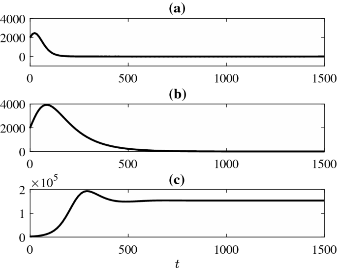
Number of infected individuals. The parameters of model and optimal control are presented in the Table 1. a Vaccination designed by optimal control (8). b Constant vaccination \(v_c = 0.40\). c Without vaccination. Notice that the same initial condition is adopted for all three cases. It is clear that the simulation performed with the optimal control presents the lowest peak of infected and the shortest time to eradicate the disease

Comparison between vaccination in three situations. Optimal Control (black dashed line). Constant vaccination (dashed dotted red line). Without vaccination (dotted blue line). The constant vaccination rate is obtained by Eq. (2) and optimal control is obtained by Eq. (8). The y-axis is the vaccination rate and x-axis is time in an arbitrary unit. From this graph it is possible to notice an interesting behaviour of the optimal control. It starts with a very high vaccination rate, which allows a sharp reduction afterwards

Comparison between cost obtained by (3) in three situations. Optimal control (black dashed line). Constant vaccination (dashed dotted red line). Without vaccination (dotted blue line). The total cost in each situation was put in a per unit system. The y-axis is the cost and x-axis is time in an arbitrary unit. In the beginning the cost of optimal control is higher, which is clearly related to an adoption of a much higher vaccination rate. However, after some time, this cost becomes lower than the cost provided by constant vaccination

Adjoint process \(p_1\). This behaviour is close related to the optimal control seen in Fig. 2
Another important feature of the application of the optimal control can be concluded from Fig. 5. Using the parameters of Table 1 and the stability analysis for the fixed point \(P_1\), an endemic state should occur when \(\beta >\gamma +\mu =0.056\). In this state, \(P_1\) is not stable and \(I>0\). We chose \(\beta\) varying from 0.056 to 0.1. The initial condition of the optimal control \(v^*(0)\) and the corresponding \(v_\mathrm {c}\) for each value of \(\beta\) are shown in Fig. 5. The initial value of the optimal control is higher than the critical value of vaccination when \(\beta\) increases. As the value of \(\beta\) is slightly greater than the minimum for many infectious diseases (see [3]), this fact can reveal an important practical orientation. The cost of vaccination campaigns can be optimized if the initial value is taken higher than the critical value for vaccination \(v_\mathrm {c}\).

Initial value of vaccination rate using the optimal control (–) and constant vaccination (-o-) for different values of \(\beta\). Notice that for \(\beta >0.06\), the vaccination rate designed by optimal control is higher than the critical value Eq. (2). It is also important to stress that in the majority of the cases the initial value is much higher. Moreover, values above 1 should be obviously saturated in 1 (maximum population cover of 100%)
Vaccination Policy Based on Optimal Control Law
As presented, optimal control is able to provide satisfactory results. However, there is not always a prior knowledge of the number of susceptible, infected, and recovered individuals required to formulate and solve the optimal control problem. Therefore, constant vaccination has been used as a way to mitigate the effects of lack of knowledge of system states, but this approach produces a very high cost when compared to the cost of applying the optimal control.
To overcome the highlighted difficulties, a vaccination policy is proposed in which prior knowledge of the states is not necessary. The proposed approach starts with a high percentage of vaccination, to emulate the optimal control action. This percentage is then reduced to half of the initial value. From this moment on pulses of vaccination with constant interval and decreasing intensity are applied until the percentage of vaccination is zero. It is important to state that if the number of infected individuals does not reach zero, a small rate of vaccination can be continued applied.
Figures 6 and 7 show the comparison of results for vaccination and cost, respectively. In each figure, there are the situations: vaccination designed by optimal control, constant vaccination, without vaccination and proposed vaccination. The total cost in each situation was put in a per-unit system.
The weight for the number of infected individuals was varied and the results are summarized in Table 2. Optimal vaccination represents the minimum cost, except for \(\phi _2 = 0.1\), when the system without vaccination represents the minimum value. As can be seen, the final cost obtained by the proposed methodology is higher than the cost obtained by the optimal control and lower than the cost obtained by constant vaccination. It is noteworthy that the states were not used to formulate the control policy, which makes the scenario more realistic in view of the lack of accurate information about the system.
An important aspect that deserves our attention is related to the possibility of a second infection. It has been reported that it is likely that people can be reinfected with COVID-19. However, the degree of protective immunity conferred by infection by COVID-19 is currently unknown [48]. It means that at this stage of scientific development it would be very hard to incorporate such variables in the dynamics of the system. Nevertheless, one of the great advantages of compartmental models is the ability to easily incorporate new state variables. As soon as it would be possible to recognise the dynamics of the system, the loss of immunity can be included. This can be done, for instance, by adapting the SIR epidemic model with partial temporary immunity, as presented in [49].

Comparison between vaccinations. Proposed control policy (full green line). Optimal Control (black dashed line). Constant vaccination (dashed dotted red line). Without vaccination (dotted blue line). The constant vaccination rate is obtained by Eq. (2) and optimal control is obtained by Eq. (8). The proposed control policy (full green line) is particularly interesting for situations where the model is unknown or there is a substantial amount of uncertainty in the data to produce a blax-box model

Comparison between cost obtained by (3). Proposed control policy (full green line). Optimal control (black dashed line). Constant vaccination (dashed dotted red line). Without vaccination (dotted blue line). The total cost in each situation was put in a per unit system. The y-axis is the cost and x-axis is time in an arbitrary unit. The performance of the Optimal Control is the best. However, it requires a precise model. Thus, the proposed policy can be an useful alternative in a model-free scenario
Conclusions
This paper has presented an optimal control law to minimize the number of infected individuals and the vaccination rate. Furthermore, the strategy considered is based on an analytic function. Some aspects have been investigated. First, the number of infected individuals is analysed. The optimal vaccination campaigns present significant differences (Fig. 1). Both methodologies guarantee eradication of the disease, but with different peaks and eradication time. Optimal control takes one third of time to eradicate the disease when compared to constant vaccination. The maximum number of infected in the case of optimal control is around 50% lower than in the case of constant vaccination. The system without vaccination stabilizes around \(1.5 \times 10^{5}\) infected individuals.
Secondly, the vaccination for the three situations are quite different, as shown in Fig. 2. The optimal vaccination starts at a higher level than the constant vaccination and decreases smoothly until it reaches zero at \(t=300\). We believe this can indicate an important principle to design vaccination campaigns. The campaign should start with a high value and then it might be reduced throughout the time (see Figs. 2 and 5). Some similar results have been reached in [50], where the authors show the importance of a great investment in the start of a campaign. Thus, a great investment in vaccination campaigns reduces the cumulative cost in the long term. From this and the fact that there is not always a prior knowledge of the number of susceptible, infected and recovered individuals required to formulate and solve the problem of optimal control, a vaccination policy was proposed in which the prior knowledge of the states is not necessary. The proposed approach starts with a high percentage of vaccination, to emulate the optimal control action. This percentage is then reduced to half of the initial value. From this moment on pulses of vaccination with constant interval and decreasing intensity are applied until the percentage of vaccination is zero (see Fig. 6). Figure 7 presents the cumulative cost for the four studied cases. The results indicate that the absence of vaccination has the highest cost in the long term. In the short-term, the total cost of the optimal control is higher than the other cases. Besides that, the final cost obtained by the proposed methodology is higher than the cost obtained by the optimal control and lower than the cost obtained by constant vaccination, noting that neither prior knowledge of the number of susceptible, infected and recovered individuals was used in this approach.
Finally, another point is that the use of Pontryagin’s maximum principle yields an analytic function for the optimal control law. Thus, this conclusion can be expanded for a more realistic scenario the persistence of an infectious disease can also be described because of this relation. Although, in general there is no optimal design for vaccination campaigns, it is clear that economic pressures can be seen as a cost function, which make governmental agencies optimize their resources, and therefore, the vaccination campaign. Another interesting possibility to investigate is related to incorporating uncertainty from data and from computer simulation using interval arithmetic approaches for nonlinear dynamical systems as in [51,52,53].
Finally, it is important to stress that under the enormous pressure that global society has been facing to fight the COVID-19 pandemic, the results pointed here are based on the optimistic perspective for the development of a vaccine [54]. There is one lesson that, unfortunately, almost all countries have not learned: be prepared for a pandemic, as has been warned by many scientists and global leaders [55]. Therefore, it is really important to start to investigate how to deal with a massive and global vaccine campaign. The results here pointed out the importance of a robust response of vaccination to a quick eradication of the COVID-19. Future works should address other compartmental models, such as SEIR [41], and specific parameters for each country or region of the globe. It would be of great interest to incorporate other techniques to forecast COVID-19 as seen in [56].
Data Availability
The simulations are generated based on the given model in the paper and no external data is used for them.
References
Hethcote HW. The mathematics of infectious diseases. SIAM Rev. 2000;42(4):599.
Murray JD. Mathematical biology, mathematical biology. Berlin: Springer; 1993.
Anderson RM, May RM. Infectious diseases of humans: dynamics and control. Oxford: Oxford University Press; 1992.
Wickwire K. Mathematical-models for control of pest and infectious-diseases - survey. Theor Popul Biol. 1977;11(2):182.
Staněk J. Kermack-McKendrick epidemics vaccinated. Kybernetika. 2008;44(5):705.
Yang J, Wang X. Threshold dynamics of an SIR model with nonlinear incidence rate and age-dependent susceptibility. Complexity. 2018;2018:1.
Nepomuceno EG, Barbosa AM, Silva MX, Perc M. Individual-based modelling and control of bovine brucellosis. R Soc Open Sci. 2018;5(5):180200.
Pinto ER, Nepomuceno EG, Campanharo ASLO. Communications in computer and information science. Berlin: Springer International Publishing; 2019. p. 81–8.
Li Y, Ye M, Zhang Q. Strong convergence of the partially truncated Euler-Maruyama scheme for a stochastic age-structured SIR epidemic model. Appl Math Comput. 2019;362:124519.
Slama H, Hussein A, El-Bedwhey NA, Selim MM. An approximate probabilistic solution of a random SIR-type epidemiological model using RVT technique. Appl Math Comput. 2019;361:144.
Walker PGT, et al. Imperial college COVID19-global impact. Imperial College COVID-19 Response Team. 2020; 1–19. https://doi.org/10.25561/77735.
Kar TK, Batabyal A. Stability analysis and optimal control of an SIR epidemic model with vaccination. Biosystems. 2011;104(2–3):127.
Huang C, Wang Y, Li X, Ren L, Zhao J, Hu Y, Zhang L, Fan G, Xu J, Gu X, et al. Clinical features of patients infected with 2019 novel coronavirus in Wuhan, China. Lancet. 2020;395(10223):497.
Mallapaty S. Why does the coronavirus spread so easily between people? Nature 2020;579:183–183
Kermack W, McKendrick A. A contribution to the mathematical theory of epidemics. Proc R Soc Lond Ser A. 1927;A115:700.
Yang FY, Li WT, Wang ZC. Traveling waves in a nonlocal dispersal SIR epidemic model. Nonlinear Anal Real World Appl. 2015;23:129.
Allen LJS. Some discrete-time SI, SIR, and SIS epidemic models. Math Biosci. 1994;124(1):83.
Rashidinia J, Sajjadian M, Duarte J, Januário C, Martins N. On the dynamical complexity of a seasonally forced discrete SIR epidemic model with a constant vaccination strategy. Complexity. 2018;2018:1.
Demongeot J, Hansen O, Hessami H, Jannot A, Mintsa J, Rachdi M, Taramasco C. Random modelling of contagious diseases. Acta Biotheor. 2013;61(1):141.
Ackleh AS, Allen LJS. Competitive exclusion and coexistence for pathogens in an epidemic model with variable population size. J Math Biol. 2003;47(2):153.
Yang W, Sun C, Arino J. Global analysis for a general epidemiological model with vaccination and varying population. J Math Anal Appl. 2010;372(1):208.
Behncke H. Optimal control of deterministic epidemics. Optim Control Appl Methods. 2000;21(6):269.
Zhou Y, Wu J, Wu M. Optimal isolation strategies of emerging infectious diseases with limited resources. Math Biosci Eng. 2013;10(5/6):1691.
Lashari AA. Optimal control of an SIR epidemic model with a saturated treatment. Appl Math Inform Sci. 2016;10(1):185.
Grigorieva EV, Khailov EN, Korobeinikov A. Optimal control for a SIR epidemic model with nonlinear incidence rate. Math Model Natl Phenom. 2016;11(4):89.
Di Giamberardino P, Iacoviello D. Optimal control of SIR epidemic model with state dependent switching cost index. Biomed Signal Process Control. 2017;31:377.
Alonso D, Bouma MJ, Pascual M. Epidemic malaria and warmer temperatures in recent decades in an East African highland. Proc Biol Sci. 2011;278(1712):1661.
Elazzouzi A, Lamrani Alaoui A, Tilioua M, Tridane A. Global stability analysis for a generalized delayed SIR model with vaccination and treatment. Adv Diff Equat. 2019;2019(1):532. https://doi.org/10.1186/s13662-019-2447-z.
Farrington CP. On vaccine efficacy and reproduction numbers. Math Biosci. 2003;185:89.
Kribs-Zaleta CM, Velasco-Hernandez JX. A simple vaccination model with multiple endemic states. Math Biosci. 2000;164:183.
Gandon S, Mackinnon M, Nee S, Read A. Imperfect vaccination: some epidemiological and evolutionary consequences. Proc R Soci Lond Ser B. 2003;270(1520):1129.
Colombo RM, Garavello M. Optimizing vaccination strategies in an age structured SIR model. Math Biosci Eng. 2020;17(2):1074.
Gersovitz M, Hammer JS. The economical control of infectious diseases. Econ J. 2004;114(492):1.
Kirk DE. Optimal control theory: an introduction. Englewood Cliffs: Prentice-Hall Inc.; 1970.
Francis PJ. Optimal tax/subsidy combinations for the flu season. J Econ Dyn Control. 2004;28(10):2037.
Ogren P, Martin CF. Vaccination strategies for epidemics in highly mobile populations. Appl Math Comput. 2002;127(2–3):261.
Briat C, Verriest EI. A new delay-SIR model for pulse vaccination. Biomed Signal Process Control. 2009;4(4):272.
Bolzoni L, Bonacini E, Soresina C, Groppi M. Time-optimal control strategies in SIR epidemic models. Math Biosci. 2017;292:86.
Das A, Pal M. A mathematical study of an imprecise SIR epidemic model with treatment control. J Appl Math Comput. 2018;56(1–2):477.
Laaroussi AEA, Rachik M, Elhia M. An optimal control problem for a spatiotemporal SIR model. Int J Dyn Control. 2018;6(1):384.
Lacerda MJ, Nepomuceno EG. ResearchGate Preprint. 2020;1:1–4.
Nepomuceno EG, Takahashi RH, Aguirre LA. Reducing vaccination level to eradicate a disease by means of a mixed control with isolation. Biomed Signal Process Control. 2018;40:83.
Momtazmanesh S, Ochs HD, Uddin LQ, Perc M, Routes JM, Vieira DN, Al-Herz W, Baris S, Prando C, Rosivall L, Abdul Latiff AH, Ulrichs T, Roudenok V, Aldave Becerra JC, Salunke DB, Goudouris E, Condino-Neto A, Stashchak A, Kryvenko O, Stashchak M, Bondarenko A, Rezaei N. All together to fight COVID-19. Am J Trop Med Hyg. 2020;102(6):1181. https://doi.org/10.4269/ajtmh.20-0281.
Moghadas SM. Analysis of an epidemic model with bistable equilibria using the Poincaré index. Appl Math Comput. 2004;149(3):689.
Pontryagin LS, Boltyanskii VG, Gamkrelidze RV, Mishchenko EF. The mathematical theory of optimal processes. New York: Wiley; 1962.
Gamarra JGP, Solé RV, Alonso D. Control, synchrony and the persistence of chaotic populations. Chaos Solitons Fractals. 2001;12:235.
Kierzenka J, Shampine LF. A BVP solver based on residual control and the MATLAB PSE. ACM Trans Math Softw. 2001;27(3):299.
Tillett RL, Sevinsky JR, Hartley PD, Kerwin H, Crawford N, Gorzalski A, Laverdure C, Verma SC, Rossetto CC, Jackson D, Farrell MJ, Van Hooser S, Pandori M. Lancet Infect Dis. 2020. https://doi.org/10.1016/S1473-3099(20)30764-7.
Taylor ML, Carr TW. An SIR epidemic model with partial temporary immunity modeled with delay. J Math Biol. 2009;59(6):841. https://doi.org/10.1007/s00285-009-0256-9.
Caetano MAL, Yoneyama T. Optimal and sub-optimal control in the dengue epidemics. Optim Control. 2001;22(2):63.
Nepomuceno EG, Martins SA, Silva BC, Amaral GF, Perc M. Detecting unreliable computer simulations of recursive functions with interval extensions. Appl Math Comput. 2018;329:408.
Peixoto ML, Nepomuceno EG, Martins SA, Lacerda MJ. Computation of the largest positive Lyapunov exponent using rounding mode and recursive least square algorithm. Chaos Solitons Fractals. 2018;112:36.
Moore RE, Kearfott RB, Cloud MJ. Introduction to interval analysis. Philadelphia: SIAM; 2009.
Kim YC, Dema B, Reyes-Sandoval A. COVID-19 vaccines: breaking record times to first-in-human trials. npj Vaccines. 2020;5(1):34.
Gates B. Responding to Covid-19 — A Once-in-a-Century Pandemic? New England J Med. 2020;382(18):1677–1679. https://doi.org/10.1056/NEJMp2003762.
Perc M, Gorišek Miksić N, Slavinec M, Stožer A. Forecasting COVID-19. Front Phys. 2020;8:5. https://doi.org/10.3389/fphy.2020.00127.
Acknowledgements
Dr. Nepomuceno received financial support from CNPq: Grant Nos. 465704/2014-0 and 425509/2018-4, and FAPEMIG: Grant No. APQ-00870-17. Luis A. Aguirre was supported by CNPq (Grant No. 302079/2011-4).
Author information
Authors and Affiliations
Corresponding author
Ethics declarations
Conflict of interest
The authors declare that there is no conflict of interest regarding the publication of this paper.
Additional information
Publisher's Note
Springer Nature remains neutral with regard to jurisdictional claims in published maps and institutional affiliations.
This article is part of the topical collection “Computer Aided Methods to Combat COVID-19 Pandemic” guest edited by David Clifton, Matthew Brown, Yuan-Ting Zhang and Tapabrata Chakraborty.
Rights and permissions
About this article

Cite this article
Nepomuceno, E.G., Peixoto, M.L.C., Lacerda, M.J. et al. Application of Optimal Control of Infectious Diseases in a Model-Free Scenario. SN COMPUT. SCI. 2, 405 (2021). https://doi.org/10.1007/s42979-021-00794-3
Received:
Accepted:
Published:
DOI: https://doi.org/10.1007/s42979-021-00794-3