Abstract
Activation functions are essential in deep learning, and the rectified linear unit (ReLU) is the most widely used activation function to solve the vanishing gradient problem. However, owing to the dying ReLU problem and bias shift effect, deep learning models using ReLU cannot exploit the potential benefits of negative values. Numerous ReLU variants have been proposed to address this issue. In this study, we propose Dynamic Parametric ReLU (DPReLU), which can dynamically control the overall functional shape of ReLU with four learnable parameters. The parameters of DPReLU are determined by training rather than by humans, thereby making the formulation more suitable and flexible for each model and dataset. Furthermore, we propose an appropriate and robust weight initialization method for DPReLU. To evaluate DPReLU and its weight initialization method, we performed two experiments on various image datasets: one using an autoencoder for image generation and the other using the ResNet50 for image classification. The results show that DPReLU and our weight initialization method provide faster convergence and better accuracy than the original ReLU and the previous ReLU variants.
1 Introduction
Deep learning has yielded state-of-the-art results in various fields, such as computer vision [33, 35], natural language processing [2, 25], public health [14, 32], biology [1, 12], and recommendation [6, 8]. These revolutionary advancements are primarily the results of several important factors, including high-level computing power, efficient artificial intelligence models, and big data technology. Among these crucial advancements, this study focused on the activation function and weight initialization in deep learning.
Activation function is an essential part of deep learning, enabling faster convergence and sparse activation by determining the depth and non-linear properties of a network [23]. The hyperbolic tangent and sigmoid have been traditionally used as activation functions [26]. The most well-known and popular activation function is the rectified linear unit (ReLU) [21], and its effectiveness has been verified in the previous studies [5, 13, 34]. ReLU mitigates the gradient vanishing problem by allowing equal propagation of all positive inputs, enabling to train deeper networks. Furthermore, ReLU has high computational efficiency as it outputs zero for negative input. However, ReLU has the disadvantages that the bias shift effect and dying ReLU problem occur owing to zero output for negative values during training [18]. To alleviate these problems, numerous ReLU variants have been proposed. Leaky ReLU (LReLU) [18] was proposed to solve the dying ReLU problem by replacing the negative part of ReLU with a linear function having a fixed negative slope, such as 0.01, to preserve a small negative signal. Parametric ReLU (PReLU) [9] is an extension of the LReLU that uses a learnable parameter, alpha (\(\alpha\)), to determine the negative slope by training, resulting in improved performance with small risk of overfitting. In addition, Flexible ReLU (FReLU) [24] was proposed to solve the bias shift effect of ReLU by determining the overall bias through training using a learnable parameter, bias.
Weight initialization is another important aspect of deep learning. It is well known that improper initialization can hamper the training of deep learning models and slow down the convergence speed, especially in deep networks [20]. Since the time that the method of weight initialization based on unsupervised pre-training was proposed [11], various studies have been conducted to initialize weights properly [3, 4]. With the emergence of sophisticated deep learning models in recent years, the Xavier initialization method was introduced. This method considers the number of nodes in a layer, under the assumption that the activation function is linear [7]. This method worked well in most cases with the existing activation functions, such as hyperbolic tangent and sigmoid, but was not applicable to ReLU. Hence, He initialization was extended from Xavier initialization [9], exhibiting excellent performance in training deep networks using ReLU as the activation function.
The motivations for this study are: (i) the formulation of ReLU can be more suitably adapted to each model and dataset; (ii) the convergence speed and accuracy of the model can be improved if its activation formulation is learned by training rather than determined by a person. Thus, we propose a novel activation function, Dynamic Parametric ReLU (DPReLU), and its proper weight initialization method, as an extended version of our previous work [19]. DPReLU can dynamically control the overall functional shape of ReLU by incorporating four trainable parameters, including \(\alpha\) of PReLU and bias of FReLU. The following are the proposed parameters of DPReLU:
-
alpha (\(\alpha\)): Determines the slope of the negative part in ReLU.
-
beta (\(\beta\)): Determines the slope of the positive part in ReLU.
-
bias: Determines the overall bias of the ReLU formulation.
-
threshold: Determines the overall threshold of the ReLU formulation.
This design makes DPReLU more flexible than previous activation functions, with only 4L additional parameters, where L is the number of activation layers. In addition, ReLU, LReLU, PReLU, and FReLU can be considered as special cases of DPReLU. Furthermore, we present a robust weight initialization method. This method is suitably derived for deep neural networks using DPReLU, based on the current theory. It allows training to converge faster, and prevents the gradient vanishing and accuracy saturation problems, even in deeper networks.
To evaluate DPReLU and the proposed weight initialization method, we performed two experiments on various image datasets (two 1-channel image datasets and three 3-channel image datasets): one using an autoencoder for image generation and the other using the ResNet50 for image classification. The performance was verified by comparing the experimental results with those of the original ReLU, PReLU, and FReLU.
The major contributions of this study are as follows:
-
We propose a novel activation function, DPReLU, which dynamically makes the overall functional shape of ReLU more flexible and suitable with four learnable parameters for each dataset and model.
-
We present an appropriate and robust weight initialization method for DPReLU, which enables faster convergence and prevents gradient vanishing and performance degradation.
-
Through experiments on various image datasets, we show that DPReLU and its weight initialization method outperform the original ReLU and its variants in terms of convergence speed and accuracy.
The remainder of this paper is organized as follows. Section 2 introduces the related work. Section 3 presents the proposed DPReLU and its proper weight initialization method. Section 4 presents the details of our experiments, and the paper is concluded in Sect. 5.
2 Related Work
In this section, we review several studies related to the proposed DPReLU and its weight initialization method.
2.1 Activation Functions
The activation function is one of the major components in deep learning that allows faster convergence and sparse activation by determining the depth and non-linear properties of networks. The hyperbolic tangent and sigmoid have been traditionally used as activation functions. Recently, various studies on activation function have been conducted. Among the various activation functions, in this subsection, we review the original ReLU and several ReLU variants that motivated to the proposed DPReLU, as shown in Fig. 1.

Illustration of the original ReLU and its variants
Rectified Linear Unit (ReLU) [21] is an essential element of deep neural networks. As shown in Eq. (1), ReLU bypasses positive inputs to keep their values unchanged and outputs zero for all negative inputs. Therefore, it can alleviate the gradient vanishing problem, enabling the training of deeper neural networks, whereas the traditional sigmoid activation function cannot. Although ReLU is an efficient activation function, it has the disadvantages of the dying ReLU problem and bias shift effect. The dying ReLU effect is where the negative signal always dies, because it outputs zero for all negative values, and bias shift can lead to oscillations and impede learning
Leaky ReLU (LReLU) [18] was proposed as an extension of ReLU to solve the dying ReLU problem. The positive part of LReLU is the same as that in ReLU, and the negative part is replaced by the product of the input and a fixed slope parameter, such as 0.01, to preserve small negative signals, as shown in Eq. (2). LReLU provides comparable performance to ReLU, but the results are sensitive to slope values
Parametric ReLU (PReLU) [9] is a variant of LReLU. As shown in Eq. (3), the fixed parameter that sets the slope of the negative part in LReLU is replaced by a learnable parameter, \(\alpha\), that is determined by training. This learnable parameter can be shared by all channels, or assigned independently to each channel in the hidden layer of a neural network. This activation function has been shown to improve the performance of convolutional neural networks in ImageNet classification with small risk of overfitting
Flexible ReLU (FReLU) [24] is a modification of ReLU proposed to mitigate the bias shift effect. In FReLU, a learnable parameter, bias, is introduced to control the bias of the overall function shape through training, as shown in Equation (4). FReLU showed better performance and faster convergence than ReLU with weak assumptions and self-adaption.
2.2 Weight Initialization
Weight initialization is another crucial part of deep learning. Weight initialization by random sampling from a Gaussian distribution with a fixed standard deviation has been traditionally used in deep learning [17]. However, this method can reduce the convergence speed and disturb the training of deep learning models, especially in deep networks [27]. This problem arises, because random initialization causes the input signal to propagate into deeper layers with a small variance, slowing down back propagation and disrupting the entire training process. Weight initialization has been studied extensively, and various methods have been proposed to deal with the problem of variance reduction in deeper layers.
Deep Belief Network (DBN) [11] is the first study of weight initialization in deep networks. Before this research, there was no suitable weight initialization method for deep networks. In DBN, all weights are initialized sequentially from the first layer using a layer-wise unsupervised pre-training algorithm [29]. This method performed better than neural networks without weight initialization, but showed drawbacks that it required more training time, and may lead to poorer local optimal in deep networks. Since then, with the advent of deeper networks, several studies have shown that deep networks still face the weight initialization problem [27, 28].
Xavier Initialization [7] allows fast convergence without the variance reduction problem in deep networks, under the assumption of linearity. In this method, weights are initialized by randomly sampling from a normal or a uniform distribution with variance of weights determined by considering the number of input and output nodes in each layer. Equation (5) shows the variance of the initialized weights by the Xavier method using the normal distribution, where W is the weights, \(n_{in}\) is the number of input nodes, and \(n_{out}\) is the number of output nodes. The initialized weights in this manner can have the same distribution across all layers, even in deeper layers. This method performed well in most cases with the existing activation functions such as hyperbolic tangent and sigmoid, but was not applicable to ReLU activation function
He Initialization [9] is the most widely used weight initialization method in recent years. This method was extended from Xavier initialization for ReLU and PReLU. In this method, the variance of the weights is obtained by simply dividing the denominator of Eq. (5) by 2, taking into account the negative part of the ReLU, as shown in Eq. (6). This method has shown good performance for training very deep networks with ReLU
3 Methodology
3.1 Dynamic Parametric ReLU (DPReLU)
In this section, we present our novel activation function, DPReLU, which can dynamically make the ReLU function more flexible and learnable during training, rather than using a fixed parameters function. The shape of DPReLU is shown in Fig. 2.

Illustration of the DPReLU
There are four additional learnable parameters compared to the vanilla ReLU. \(\alpha\) and \(\beta\) are the slopes of the negative and positive parts in the function, respectively. Here, a negative or positive case is determined when comparing input x to the threshold. The threshold makes DPReLU shift on the x-axis in comparison to the original ReLU. The bias determines the alignment of the function with respect to the y-axis. These four parameters are all learnable and interact with each other during the training phase. In addition, ReLU, LReLU, PReLU, and FReLU can be considered as special cases of DPReLU. When \(\alpha = 0\), \(\beta = 1\), \(threshold = 0\), and \(bias = 0\), the DPReLU becomes the vanilla ReLU. DPReLU has more learnable parameters than the PReLU, which only has \(\alpha\), and the FReLU, which only has bias. The overall formula of DPReLU is shown in Eq. (7)
3.2 Weight Initialization
In this section, we present the derivation of our weight initialization method for DPReLU. In our method, weights are initialized by randomly sampling from a normal distribution with appropriate variance across all layers. Our derivation mainly follows the Xavier and He initialization methods [7, 9].
In forward propagation, a layer in a neural network is commonly computed by: \(y_l\) = \(W_lx_l+b_l\), where \(y_l\) is the output vector of dimension m-by-1, \(x_l\) is an input vector of dimension n-by-1, \(W_l\) is a weight matrix of dimension n-by-m, and \(b_l\) is a bias vector. We assume that the initialized elements in \(W_l\) are independent of each other and share the same distribution. Similarly, we assume that the elements in \(x_l\) are also independent of each other and share the same distribution, and \(x_l\) and \(W_l\) are independent of each other. Then, we can obtain \(Var[y_l]\) = \(nVar[W_l]E[x_{l}^{2}]\) from the above equation. If we let \(W_l\) and \(x_l\) follow a normal distribution that is symmetric around zero and has zero mean, this leads to \(E[x^{2}_l]\) = \(\frac{\alpha ^2}{2}Var[y_{l-1}]+\frac{\beta ^2}{2}Var[y_{l-1}]\) when the activation function is DPReLU. In this, we set the threshold and bias to 0 for convenience of derivation. Substituting this into the above equation, we have \(Var[y_l]=\frac{\alpha ^2+\beta ^2}{2}nVar[W_l]Var[y_{l-1}]\). This equation is the key of initialization method. For proper weight initialization, \(Var[y_l]\) and \(Var[y_{l-1}]\) should be equal to avoid variance reduction problems. Thus, a sufficient initialization condition is obtained, as shown in Eq. (8), where \(n_{in}\) is the number of input nodes
For backward propagation, the weight initialization condition can be simply derived in the same manner as in the forward propagation case, as shown in Eq. (9), where \(n_{out}\) is the number of output nodes
In conclusion, to consider both forward and backward propagation cases, the average of Eqs. (8) and (9) is used as the weight initialization condition in all experiments, as shown in Eq. (10)
4 Experiments
In this section, we explain the details of our experimental setup and the results for the autoencoder and image classification experiments on various datasets.
4.1 Autoencoder for Image Reconstruction
In this experiment, we employed an autoencoder model and applied different activation functions and weight initialization methods to compress and reconstruct images. An autoencoder is composed of two parts: an encoder and a decoder. The goal of autoencoders is to represent the input in a latent space (by the encoder) and reconstruct the original input from that latent representation (by the decoder). The loss function used in this experiment is the mean square error (MSE) between the input and reconstructed images.
For this experiment, we selected two 1-channel image datasets and three 3-channel datasets. The 1-channel image datasets are MNIST [16] and FashionMNIST [31]. Each dataset contains 60,000 28×28 gray-scaled images, 50,000 for training and 10,000 for testing. For these datasets, we applied a fully connected layer-based autoencoder. The encoder comprises four fully connected layers with 1000, 500, 250, and 30 units, respectively (the latent representation dimension is 30). The decoder is symmetrical to the encoder in reconstructing the input image. Apart from the last layer of the encoder and decoder, each layer is followed by a ReLU variant activation. The activation for the last layer of the decoder is the sigmoid function, because we aim to reconstruct the image pixels with values ranging from 0 to 1, similar to the input images. The detailed architecture is shown in Table 1.
For 3-channel image datasets, we used the CIFAR-10, CIFAR-100, and SVHNcropped datasets [15, 22]. The CIFAR datasets contain 50,000 and 10,000 32x32 color images for training and testing, respectively. SVHNcropped dataset contains 73,257 and 26,032 32×32 color images for training and testing, respectively. These datasets contain 3-channel images; hence, we adopted convolutional layers in the model rather than just fully connected layers. Unlike the autoencoder for 1-channel image datasets, the encoder comprises two convolutional layers with 64 and 128 filters, kernel size of 3, and stride of 2. Subsequently, there are two fully connected layers with 1024 and 30 units (the latent representation dimension is 30). The decoder is symmetric to the encoder and contains convolutional transpose layers to reconstruct the original shape of the image. Except for these, the rest of the structures are the same as the autoencoder for 1-channel image datasets, and the details are shown in Table 2.
The activations applied in this experiment (the ‘Activation‘ term in Tables 1 and 2) were the vanilla ReLU, PReLU, FReLU, and DPReLU (our approach). In the cases of PReLU, FReLU, and DPReLU, each filter in a convolutional layer (channel-wise) and each unit in a fully connected layer (element-wise) had its own activation parameters. The initial bias of FReLU was the same as ReLU, while PReLU was initialized with \(\alpha \in \{0, 0.1, 0.25, 0.5\}\). DPReLU was initialized with \(\alpha \in \{0, 0.1, 0.25, 0.5\}\) and \(\beta \in \{0.5, 0.75, 0.9, 1\}\) (16 experiments). For bias and threshold of DPReLU, both initial values were set to 0. Hereafter, if not specified, \(\alpha\)=0 means that \(\alpha\) was initialized as 0.
In addition, we applied different weight initialization approaches for the autoencoder models. For the models using ReLU, PReLU, and FReLU, we used He initialization was as originally proposed [9, 24]. For the model using DPReLU, our approach proposed in 3.2 was used. The two methods obtained weights following normal distribution with the same \(\mu\)=0. The difference lies in the variance (\(\sigma ^2\)) of the weights in each layer, as follows:
-
He initialization: \(Var(w) = \frac{4}{(n_{in} + n_{out}) * (1 + \alpha ^2)}\)
(The value of \(\alpha\) is 0 for ReLU and FReLU)
-
Our approach: \(Var(w) = \frac{4}{(n_{in} + n_{out}) * (\alpha ^2 + \beta ^2)}\).
The models were trained with the Adam optimizer, a learning rate of \(1e-5\), and a batch size of 128. All experiments were conducted on a machine using two NVIDIA TITAN RTX 24GB graphic cards. To evaluate the quality of the reconstruction, the following metrics were used: Mean Square Error (MSE), Peak Signal-to-Noise Ratio (PSNR), and Structural SIMilarity (SSIM). These metrics were mainly used to evaluate the quality of the generated images [30]. We selected well-performed results by grid-search, and the results are reported in Table 3 and Fig. 3.

Performance of the autoencoder models using each activation with corresponding weight initialization from 5th to 50th epoch on various image datasets. (\(\alpha\) and \(\beta\) represent the initial values that performed the best in each model, which changed dynamically during training.)
Figure 3 shows the training MSE, testing MSE, testing PSNR, and testing SSIM between the input and reconstructed images, when training the autoencoder model using different activation functions with corresponding weight initialization, on various datasets. We reported from 5th to 50th epoch for readable visualization.
Overall, the same downward pattern of the MSE and the same upward pattern of PSNR and SSIM can be observed in the figures for all activation functions on all datasets. In the case of 1-channel datasets, all models using different activation functions tended to converge to similar values, especially in the SSIM of MNIST and all metrics of FashionMNIST [Fig. 3(A)(B)]. Nevertheless, the model using DPReLU with our initialization method decreased MSE and increased PSNR and SSIM faster than the models with other activation functions on both datasets. Moreover, the DPReLU exhibited the lowest MSE and the highest PSNR on both datasets, as shown in Table 3. In the case of SSIM, the model using ReLU with He initialization was slightly higher than other models on MNIST (approximately a difference of 0.0008 from the model using DPReLU), and the model using FReLU with He initialization was slightly better than other models on FashionMNIST (approximately a difference of 0.0003 from the model using DPReLU).
For results of the 3-channel image datasets, there was a clear gap between our model and others across all metrics in all datasets over the entire training time [Fig. 3(C)(D)(E)]. The model using DPReLU with our initialization approach was able to reduce the MSE and increase the PSNR and SSIM faster than the other models, resulting in the best scores in all metrics for all datasets, as shown in Table 3.
Through these results, it is indicated that the shape of DPReLU was trained more suitably for each dataset than others in both the fully connected layer-based as well as the convolutional layer-based autoencoders, resulting in better performance including convergence speed.
4.2 ResNet for Image Classification
Image classification is a popular task in the field of computer vision. We performed image classification with the same datasets as above. The CIFAR-100 dataset consists of images of 100 classes, while the other datasets consist of images of ten classes. These five datasets have exactly the same distribution of each class in both the training and test sets.
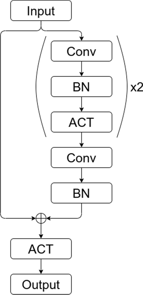
Residual block in ResNet50. (Conv: convolutional layer, BN: batch normalization layer, and ACT: ACTivation layer)
We utilized the ResNet50 model [10] using the Tensorflow framework.Footnote 1 The residual block of the model is illustrated in Fig. 4. We removed all batch normalization layers (BN), and used different functions for the activation layers (ACT). The output layer can be interpreted as the unnormalized probability that an input image belongs to a particular class. The weights of each model were initialized using various strategies, including Xavier [7], He [9], and our approach, and the performance of each strategy was compared. We did not consider batch normalization and data augmentation to assess the effect of the activation and weight initialization.
Regarding weight initialization, all methods sampled weights following the normal distribution with the same \(\mu\)=0. The difference lies in the variance (\(\sigma ^2\)) of the weights in each layer, as follows:
-
Xavier initialization: \(Var(w) = \frac{2}{n_{in} + n_{out}}\).
-
He initialization: \(Var(w) = \frac{4}{(n_{in} + n_{out}) * (1 + \alpha ^2)}\)
(The value of \(\alpha\) is 0 for ReLU and FReLU).
-
Our approach: \(Var(w) = \frac{4}{(n_{in} + n_{out}) * (\alpha ^2 + \beta ^2)}\)
(The value of \(\alpha\) is 0 for ReLU and FReLU, and the value of \(\beta\) is 1 for ReLU, PReLU, and FReLU.)
We trained the model with the Adam optimizer, categorical cross-entropy loss function, and a batch size of 128, for all datasets. The learning rate was initialized at \(1e-4\) and \(1e-3\) for the 1-channel datasets and the 3-channel datasets, respectively, and decreased by 10 times after first 10 and 20 epochs. In particular, in the case of 1-channel datasets, the original images were duplicated into 3-channels to train with the same model architecture. Furthermore, it should be noted that we ignored softmax activation when computing the output of the last layer and only used it when computing the loss for numerical stability.Footnote 2
The activations used for this experiment were ReLU, PReLU, FReLU, and DPReLU (our approach). For PReLU, FReLU, and DPReLU, the activation parameters were shared for each layer of activation (layer-wise). In other words, an activation layer used the same parameters of the activation function for all width, height, and channel dimensions. The initial bias of FReLU was same as ReLU; meanwhile, PReLU was initialized with \(\alpha \in \{0, 0.1, 0.25, 0.5\}\). DPReLU was initialized with \(\alpha \in \{0, 0.1, 0.25, 0.5\}\) and \(\beta \in \{0.5, 0.75, 0.9, 1\}\) (16 experiments). In the case of bias and threshold of DPReLU, both initial values were set to 0. We selected well-performed results by grid-search and are reported it in Fig. 5 and Table 4. The experiment was run on a machine using two NVIDIA TITAN RTX 24GB graphic cards. The source code is available on Github.Footnote 3

Performance of the ResNet50 models using each activation with the weight initialization that performed the best on various image datasets. (5th epoch \(\sim\) 50th epoch) (\(\alpha\) and \(\beta\) represent the initial values that performed the best in each model, which changed dynamically during training.)
The results of the image classification experiment are presented in Fig. 5 and Table 4. Figure 5 shows the training loss, training accuracy, and testing accuracy during training of the ResNet50 model using different activation functions with the best-performing weight initialization from 5th to 50th epoch. In addition, Table 4 illustrates the best testing accuracy of those models in numbers.
According to Fig. 5, the same downward pattern of the loss and the same upward pattern of accuracy can be observed for all activation functions on all datasets. On the MNIST dataset, although training loss and training accuracy of all models converged at similar level, the model using DPReLU with our initialization method showed faster convergence. Moreover, the DPReLU exhibited the highest score in terms of testing accuracy [Fig. 5(A)]. In the case of FashionMNIST dataset, the models using PReLU and DPReLR presented a similar trend and faster convergence than the models using ReLU and FReLU with He initialization in training loss and training accuracy. In contrast, in the testing accuracy, a clear gap in performance of each model can be observed, and the model with DPReLU outperformed the others [Fig. 5(B)].
Moving to the 3-channel image datasets, the model using DPReLU showed the fastest convergence, and the model using PReLU was the second fastest with a slightly slower speed, in terms of training loss and training accuracy of all three datasets [Fig. 5(C)(D)(E)]. In the testing accuracy, each model using different activation function showed a clear performance gap, and the model using DPReLU consistently showed the highest scores after 10th epoch on all three datasets.
Regarding the best testing accuracy of all activations with different initializations, the model using DPReLU with our initialization achieved the highest accuracy on all datasets, as shown in Table 4. In the CIFAR-100, the highest accuracy on the test set was achieved by the model that used DPReLU activation and our initialization strategy with \(\alpha\) and \(\beta\) initialized to 0.5 and 0.75, respectively. The accuracy was approximately 3% higher than that of the model using PReLU and He initialization with the \(\alpha\) initialized to 0.5, and approximately 10% higher than FReLU and ReLU. For other datasets, the models using DPReLU activation with \(\alpha\) and \(\beta\) initialized to 0.5 and 0.9, respectively, exhibited the best testing accuracy. The accuracies were slightly higher than that of the models using PReLU, and approximately 0.1%\(\sim\)7% higher than FReLU and ReLU.
4.3 Ablation Study
We now compare the performance of our initialization, Xavier, and He for the model using DPReLU activation with different initial values of \(\alpha\) and \(\beta\) on the CIFAR-10. The results are shown in Table 5.
Overall, our approach yielded stable results for most combinations of initial values of \(\alpha\) and \(\beta\), even when either Xavier or He (or both) initialization exhibited poor performance. For He initialization, the overall performance was lower than that of our initialization method. However, when the positive slope of the DPReLU was initialized close to 1 (\(\beta\)=1), it showed relatively stable performance. Note that with \(\beta = 1\), our initialization is same as He initialization. In other words, He initialization considers only the negative slope of DPReLU when initializing the model’s weights, whereas our method considers both the positive slope and negative slope that change dynamically during training. Therefore, the model using our method can perform better than the model using He initialization. In addition, the model using Xavier initialization, which considers only the number of input and output nodes, consistently performed lower than He and our method for most combinations of initial values of \(\alpha\) and \(\beta\).
For the models using other activation functions, it should be noted from the results that the performance of He initialization is better for ReLU activation than Xavier initialization. Models using He initialization outperformed those using Xavier initialization in cases of ReLU, FReLU, and PReLU on all datasets. This result is consistent with the explanation and experiments reported previously [9, 24].
Furthermore, we performed additional ablation study to analyze the contribution of each learnable parameter of DPReLU. Table 6 presents the testing accuracy of ablations performed by removing each learnable parameter of DPReLU on CIFAR-10 dataset. Removing \(\alpha\) from DPReLU resulted in the most significant drop of 0.83%, from 76.46 to 75.63%. When we removed \(\beta\), there was a 0.69% drop, from 76.46 to 75.77%. In addition, when bias or threshold was removed, a relatively low-performance degradation of 0.42% and 0.30% was observed, respectively. These ablations show that the \(\alpha\) plays the most significant role in DPReLU, followed by \(\beta\), and that bias and threshold have relatively row contributions.
Additionally, we present training process of DPReLU’s four learnable parameters in Table 7 and Fig. 6. Figure 6 shows training process of DPReLU’s four learnable parameters for each layer of ResNet50 trained on CIFAR-10, and Table. 7 shows the values of learnable parameters for each layer at epoch point showing the best test accuracy. All parameters of each layer started from their respective initial values (\(\alpha\):0.5, \(\beta\):0.9, bias:0, and threshold:0) and converged to different values. The \(\alpha\) in the shallow layers and deep layers converged to values close to the initial value, while the \(\alpha\) in the middle layers converged to values similar to the negative slope of the original ReLU. In the case of \(\beta\), they converged to different values ranging from 0.6691 to 0.9540 for each layer. The bias and threshold converged to values similar to those of the original ReLU, showing a relatively small difference for each layer. Through these, it can be considered that each layer requires different values for each parameter of DPReLU to obtain better performance.

Training process of DPReLU’s four learnable parameters for each layer of ResNet50 trained on CIFAR-10 from 0th to 50th epoch. (\(\alpha\), \(\beta\), bias, and threshold were initialized to 0.5, 0.9, 0, and 0, respectively.)
Our findings support the assumption that the parameters of ReLU can be learned via training. With the corresponding initial values of \(\alpha\) and \(\beta\), our empirical results suggest that the DPReLU activation function with our initialization strategy can further improve the performance of the model through the dynamic interaction of learnable parameters.
4.4 Running Time
Table 8 lists the number of parameters and the elapsed time for each ResNet50 model using different activation functions on the CIFAR-100 dataset. There are four additional learnable parameters for each activation layer in the case of DPReLU, and it required approximately 19 s for the model to finish an epoch. In other cases, the models ran an epoch approximately 4–7 s faster. Note that the running time may vary depending on the deep learning framework and GPU machine.

Training and testing accuracies of the ResNet50 models using each activation with corresponding weight initialization on the CIFAR-100 dataset. (0th epoch \(\sim\) 50th epoch) (\(\alpha\) and \(\beta\) represent the initial values that performed the best in each model, which changed dynamically during training.)
Figure 7 shows the accuracy of the ResNet50 model using ReLU, PReLU, FReLU, and DPReLU on the CIFAR-100 training and test sets from 0th epoch to 50th epoch. Although the running time for each epoch of the model using DPReLU is higher, its accuracy increased faster in terms of epoch and reached the highest point. For instance, it took about 7 epochs for DPReLU’s model to surpass 40% on the test set, but it took more epochs for the others. Hence, the total running time can be unchanged or reduced compared to other activations. Note that there was an increase in the accuracy of all models around the 10th epoch due to the change in the learning rate.
5 Conclusion and Future Work
Activation function is an indispensable part of deep learning models. Several studies have been conducted to improve the performance of the ReLU activation. This paper proposed a novel activation function, DPReLU, which dynamically makes the overall functional shape of ReLU more flexible and suitable for each dataset and model with four learnable parameters. In addition to the activation function, we presented a weight initialization strategy that worked for our DPReLU. We applied the DPReLU activation function and our weight initialization method to autoencoder and image classification tasks on various datasets. The proposed method outperformed ReLU and ReLU variants in terms of loss, convergence speed, and accuracy. Specifically, in the autoencoder task, the reconstruction error of the model using our method was lower and decreased faster. In the image classification task, our DPReLU and weight initialization showed stable performances, and were able to achieve the highest accuracy on various image datasets. Although the elapsed time for each epoch of the model using DPReLU is longer, the total running time is not a big concern if the number of epochs is small. However, the performances of the models using DPReLU were sensitive to the initial values of \(\alpha\) and \(\beta\). Therefore, further research is required to properly set the initial values for DPReLU. Through these results, we are able to elucidate our assumption that a learnable activation and appropriate initialization method with suitable initial values can further improve the performance of the model, especially in deep networks. Furthermore, the superiority of the proposed DPReLU has already been verified by achieving the state-of-the-art performance in light-weight model task (Zhang et al. [35]). In addition, we plan to perform further verification for a variety of applications, including natural language processing, public health, and biology in future. We believe that the proposed method has the potential to be applied to many other deep learning tasks that require deeper networks.
Data Availability
Not applicable.
Code Availability
The source code is available on Github (https://github.com/KienMN/Activation-Experiments.).
Abbreviations
- (DP)ReLU:
-
(Dynamic parametric) rectified linear unit
- LReLU:
-
Leaky ReLU
- PReLU:
-
Parametric ReLU
- FReLU:
-
Flexible ReLU
- DBN:
-
Deep belief network
- MSE:
-
Mean square error
- FC:
-
Fully connected layer
- Conv:
-
Convolutional layer
- F:
-
The number of filters
- KS:
-
Kernel size
- S:
-
Stride
- PSNR:
-
Peak signal-to-noise ratio
- SSIM:
-
Structural SIMilarity
- BN:
-
Batch normalization layer
- ACT:
-
ACTivation layer
- Init.:
-
Initialization
- s:
-
Seconds
- GPU:
-
Graphics processing unit
- \(\alpha\) :
-
Alpha
- \(\beta\) :
-
Beta
- bi :
-
Bias
- th :
-
Threshold
References
Baek, M., DiMaio, F., Anishchenko, I., Dauparas, J., Ovchinnikov, S., Lee, G.R., Wang, J., Cong, Q., Kinch, L.N., Schaeffer, R.D., et al.: Accurate prediction of protein structures and interactions using a three-track neural network. Science 373(6557), 871–876 (2021)
Barba, E., Procopio, L., Navigli, R.: ConSec: Word sense disambiguation as continuous sense comprehension. In: Proceedings of the 2021 Conference on Empirical Methods in Natural Language Processing, pp. 1492–1503 (2021)
Bengio, Y., Lamblin, P., Popovici, D., Larochelle, H.: Greedy layer-wise training of deep networks. In: Advances in neural information processing systems, pp. 153–160 (2007)
Erhan, D., Manzagol, P.A., Bengio, Y., Bengio, S., Vincent, P.: The difficulty of training deep architectures and the effect of unsupervised pre-training. In: Artificial Intelligence and Statistics, pp. 153–160 (2009)
Foret, P., Kleiner, A., Mobahi, H., Neyshabur, B.: Sharpness-aware minimization for efficiently improving generalization. In: International Conference on Learning Representations (2020)
Fu, B., Zhang, W., Hu, G., Dai, X., Huang, S., Chen, J.: Dual side deep context-aware modulation for social recommendation. In: Proceedings of the Web Conference 2021, pp. 2524–2534 (2021)
Glorot, X., Bengio, Y.: Understanding the difficulty of training deep feedforward neural networks. In: Proceedings of the thirteenth international conference on artificial intelligence and statistics, pp. 249–256 (2010)
Han, S.C., Lim, T., Long, S., Burgstaller, B., Poon, J.: Glocal-K: Global and local kernels for recommender systems. In: Proceedings of the 30th ACM International Conference on Information & Knowledge Management, pp. 3063–3067 (2021)
He, K., Zhang, X., Ren, S., Sun, J.: Delving deep into rectifiers: Surpassing human-level performance on imagenet classification. In: Proceedings of the IEEE International Conference on Computer Vision, pp. 1026–1034 (2015)
He, K., Zhang, X., Ren, S., Sun, J.: Deep residual learning for image recognition. In: Proceedings of the IEEE Conference on Computer Vision and Pattern Recognition, pp. 770–778 (2016)
Hinton, G.E., Osindero, S., Teh, Y.W.: A fast learning algorithm for deep belief nets. Neural Comput. 18(7), 1527–1554 (2006)
Jumper, J., Evans, R., Pritzel, A., Green, T., Figurnov, M., Ronneberger, O., Tunyasuvunakool, K., Bates, R., Žídek, A., Potapenko, A., et al.: Highly accurate protein structure prediction with alphafold. Nature 596(7873), 583–589 (2021)
Khosla, P., Teterwak, P., Wang, C., Sarna, A., Tian, Y., Isola, P., Maschinot, A., Liu, C., Krishnan, D.: Supervised contrastive learning. Adv. Neural Inform. Process. Syst. 33, 18661–18673 (2020)
Kim, J.K., Bae, M.N., Lee, K., Kim, J.C., Hong, S.G.: Explainable artificial intelligence and wearable sensor-based gait analysis to identify patients with osteopenia and sarcopenia in daily life. Biosensors 12(3), 167 (2022)
Krizhevsky, A., Hinton, G., et al.: Learning multiple layers of features from tiny images. Master’s thesis, Department of Computer Science, University of Toronto (2009)
LeCun, Y.: The mnist database of handwritten digits. https://www.tensorflow.org/datasets/catalog/mnist (1998)
LeCun, Y.A., Bottou, L., Orr, G.B., Müller, K.R.: Efficient backprop. In: Neural networks: tricks of the trade, pp. 9–48. Springer (2012)
Maas, A.L., Hannun, A.Y., Ng, A.Y.: Rectifier nonlinearities improve neural network acoustic models. In: Proc. ICML, vol. 30, p. 3 (2013)
Mai Ngoc, K., Yang, D., Shin, I., Kim, H., Hwang, M.: Dprelu: Dynamic parametric rectified linear unit. In: The 9th International Conference on Smart Media and Applications, pp. 121–125 (2020)
Mishkin, D., Matas, J.: All you need is a good init. arXiv preprint arXiv:1511.06422 (2015)
Nair, V., Hinton, G.E.: Rectified linear units improve restricted boltzmann machines. In: ICML’10: Proceedings of the 27th International Conference on International Conference on Machine Learning, pp. 807–814 (2010)
Netzer, Y., Wang, T., Coates, A., Bissacco, A., Wu, B., Ng, A.Y.: Reading digits in natural images with unsupervised feature learning. In: NIPS Workshop on Deep Learning and Unsupervised Feature Learning (2011)
Nwankpa, C., Ijomah, W., Gachagan, A., Marshall, S.: Activation functions: Comparison of trends in practice and research for deep learning. arXiv preprint arXiv:1811.03378 (2018)
Qiu, S., Xu, X., Cai, B.: FReLU: Flexible rectified linear units for improving convolutional neural networks. In: 2018 24th International Conference on Pattern Recognition (ICPR), pp. 1223–1228. IEEE (2018)
Ronran, C., Lee, S., Jang, H.J.: Delayed combination of feature embedding in bidirectional lstm crf for ner. Appl. Sci. 10(21), 7557 (2020)
Sharma, S.: Activation functions in neural networks. Towards Data Science 6(12), 310–316 (2017)
Simonyan, K., Zisserman, A.: Very deep convolutional networks for large-scale image recognition. arXiv preprint arXiv:1409.1556 (2014)
Szegedy, C., Liu, W., Jia, Y., Sermanet, P., Reed, S., Anguelov, D., Erhan, D., Vanhoucke, V., Rabinovich, A.: Going deeper with convolutions. In: Proceedings of the IEEE conference on computer vision and pattern recognition, pp. 1–9 (2015)
Teh, Y.W., Hinton, G.E.: Rate-coded restricted Boltzmann machines for face recognition. Adv. Neural Inform. Process. Syst. 13, 908–914 (2000)
Wang, X., Yu, K., Wu, S., Gu, J., Liu, Y., Dong, C., Qiao, Y., Change Loy, C.: Esrgan: Enhanced super-resolution generative adversarial networks. In: Proceedings of the European conference on computer vision (ECCV) workshops (2018)
Xiao, H., Rasul, K., Vollgraf, R.: Fashion-mnist: a novel image dataset for benchmarking machine learning algorithms. arXiv preprint arXiv:1708.07747 (2017)
Yang, D., Hwang, M.: ADADL: Automatic dementia identification model based on activities of daily living using smart home sensor data. In: The Thirty-Sixth AAAI Conference on Artificial Intelligence (AAAI-2022), Workshop: Trustworthy AI for Healthcare (2022)
Yang, D., Mai Ngoc, K., Shin, I., Lee, K.H., Hwang, M.: Ensemble-based out-of-distribution detection. Electronics 10(5), 567 (2021)
Yang, D., Shin, I., Kien, M.N., Kim, H., Yu, C., Hwang, M.: Out-of-distribution detection based on distance metric learning. In: The 9th International Conference on Smart Media and Applications, pp. 214–218 (2020)
Zhang, Y., Zhang, Z., Lew, L.: PokeBNN: A binary pursuit of lightweight accuracy. In: Proceedings of the IEEE/CVF Conference on Computer Vision and Pattern Recognition (2022)
Acknowledgements
This research was supported by Korea Institute of Science and Technology Information (KISTI).
Funding
This research was funded by Korea Institute of Science and Technology Information (KISTI).
Author information
Authors and Affiliations
Contributions
DY (Equal contribution): conceptualization, experiment, validation, and writing manuscript; KMN (Equal contribution): implementation, experiment, and writing manuscript; IS: conceptualization and validation; MH (Corresponding author): supervision and conceptualization.
Corresponding author
Ethics declarations
Conflict of interest
The authors declare that they have no conflict of interest.
Additional information
Publisher's Note
Springer Nature remains neutral with regard to jurisdictional claims in published maps and institutional affiliations.
Rights and permissions
Open Access This article is licensed under a Creative Commons Attribution 4.0 International License, which permits use, sharing, adaptation, distribution and reproduction in any medium or format, as long as you give appropriate credit to the original author(s) and the source, provide a link to the Creative Commons licence, and indicate if changes were made. The images or other third party material in this article are included in the article's Creative Commons licence, unless indicated otherwise in a credit line to the material. If material is not included in the article's Creative Commons licence and your intended use is not permitted by statutory regulation or exceeds the permitted use, you will need to obtain permission directly from the copyright holder. To view a copy of this licence, visit http://creativecommons.org/licenses/by/4.0/.
About this article

Cite this article
Yang, D., Ngoc, K.M., Shin, I. et al. DPReLU: Dynamic Parametric Rectified Linear Unit and Its Proper Weight Initialization Method. Int J Comput Intell Syst 16, 11 (2023). https://doi.org/10.1007/s44196-023-00186-w
Received:
Accepted:
Published:
DOI: https://doi.org/10.1007/s44196-023-00186-w