Abstract
Advanced persistent threat (APT) attacks are malicious and targeted forms of cyberattacks that pose significant challenges to the information security of governments and enterprises. Traditional detection methods struggle to extract long-term relationships within these attacks effectively. This paper proposes an APT attack detection model based on graph convolutional neural networks (GCNs) to address this issue. The aim is to detect known attacks based on vulnerabilities and attack contexts. We extract organization-vulnerability relationships from publicly available APT threat intelligence, along with the names and relationships of software security entities from CVE, CWE, and CAPEC, to generate triple data and construct a knowledge graph of APT attack behaviors. This knowledge graph is transformed into a homogeneous graph, and GCNs are employed to process graph features, enabling effective APT attack detection. We evaluate the proposed method on the dataset constructed in this paper. The results show that the detection accuracy of the GCN method reaches 95.9%, improving by approximately 2.1% compared to the GraphSage method. This approach proves to be effective in real-world APT attack detection scenarios.
Find the latest articles, discoveries, and news in related topics.Avoid common mistakes on your manuscript.
1 Introduction
With the rapid development of information technology, the volume of information in modern society continues to grow, and network threats are becoming increasingly severe. Network attacks are evolving in a new direction, with Advanced Persistent Threat (APT) attacks gradually becoming one of the primary methods of cyberattacks. APT refers to covert, persistent, and effective attack activities conducted by an organization against specific targets [1,2,3]. These attacks typically have commercial or political motivations and involve continuous monitoring of specific organizations or countries, ultimately leading to information theft or targeted disruptions, posing a significant threat to nations and enterprises’ information systems and data security [4,5,6,7]. Therefore, the detection of APT attacks has become a research hotspot in the field of network security. APT attacks exhibit strong concealment, long duration, high specificity, and significant harm. Traditional detection methods, such as malicious traffic detection, malicious code detection and log anomaly detection [8,9,10], often focus on specific phases of APT attacks and cannot detect unknown attacks. They also struggle to extract contextual correlations within APT attacks, resulting in a high false positive rate.
However, APT threat intelligence often simplifies the description of the attack process, while the vulnerabilities, weaknesses, and attack methods exploited by APT organizations make systems more susceptible to attacks [11, 12]. Therefore, inferring the vulnerabilities, related vulnerabilities, and mitigation measures used by APT from software security databases is necessary. However, associating with software security entities can enhance APT attack detection due to the lack of direct and tight correlations between individual APT threat intelligence reports, the hidden nature of software security entities, and their relationships within document content and hyperlinks. In response to this issue, recent research in APT attack detection suggests that utilizing knowledge graphs to capture rich attack context information and establish associations effectively is the optimal approach to achieve APT attack detection [13, 14].
To this end, this paper investigates a deep learning-based APT attack detection method that establishes deep associations among software security entities through a knowledge graph. Leveraging the structure of the knowledge graph, we employ Graph Convolutional Neural Networks (GCNs) to construct an APT attack detection model. GCNs excel in learning entity relationship representations within knowledge graphs, enabling the consideration of relationships between APT attacks and software security databases. This involves embedding multi-modal entity attributes and relationship attribute features of attack context into a unified low-dimensional feature space to enhance detection accuracy.
There are three contributions of our paper:
-
1.
For the first time, it generates triple data by extracting organization-vulnerability relationships from APT threat intelligence and software security entity names and relationships from Common Vulnerabilities and Exposures (CVE), Common Weakness Enumeration (CWE), and Common Attack Pattern Enumeration and Classification (CAPEC). This data is used to create a knowledge graph of APT attack behaviors.
-
2.
This paper introduces a novel GCN-based APT attack detection method that utilizes a Graph Convolutional Neural Network model to detect APT attacks and characterizes APT detection performance metrics.
-
3.
It conducts creative experiments using the Graph Convolutional Neural Network model to detect attacks such as APT-32, employing multiple performance metrics to validate the model’s effectiveness and demonstrate the superiority of Graph Convolutional Neural Networks.
The remaining sections of this paper are organized as follows: Sect. 2 discusses related research on APT attack detection. Section 3 presents the proposed method as an overall framework, briefly covering the entire process. Section 4 introduces the GCN-based APT attack detection method, including constructing the APT attack behavior knowledge graph and Graph Convolutional Neural Networks theory, accompanied by formulas and flowcharts. In Sect. 5, the method’s performance and efficiency are tested and verified, with results presented in graphs and tables. Finally, Sect. 6 concludes the paper and provides insights into future work.
2 Related Work
In the field of APT attack detection, existing research predominantly attempts to detect APT attacks based on manually defined rules using knowledge of network defense. For instance, PrioTracker [15] analyzes APT attacks using the priority of abnormal causal relationships, where the priority of system events is measured according to predefined rules. SLEUTH [16] identifies system entities and events most likely involved in APT attacks through a tag-based approach. It first encodes the credibility and sensitivity of code and data and then designs network attack detection rules using these tags. HOLMES [17] is a hierarchical framework for APT attack detection, with a critical component being an intermediate layer that maps low-level audit data to suspicious behavior using rules based on domain knowledge (such as the ATT &CK knowledge base [18]). CONAN [19] is a state-based framework where each system entity (e.g., processes or files) is represented using a structure similar to finite state automata (FSA), with states inferred based on predefined rules. The state sequences are then used for APT attack detection and reconstruction. Rule-based detection strategies have advantages such as high accuracy, strong interpretability, and ease of deployment. However, rule-based detection has limitations. First, it relies on known features, making capturing new types of APT attacks difficult. Second, it can only detect known attacks, making it challenging to identify unknown attacks or zero-day vulnerabilities where attackers exploit new vulnerabilities or attack techniques to evade existing rule-based detection. Third, it lacks context information and cannot associate multiple seemingly unrelated APT reports and software security entities to form a comprehensive threat graph.
On the other hand, learning-based techniques (including machine learning and deep learning) can automatically build APT detection models from training datasets. For example, Barre et al. [20] used trace graphs to extract features such as the total amount of written data and the number of system files used to construct a classifier for APT attack detection. Berrada et al. [21] extracted Boolean features from trace graphs and treated APT attack detection as an anomaly detection task using unsupervised learning techniques. Xiang et al. [22] extracted different features from PC and mobile platforms and employed various machine-learning algorithms to perform APT attack detection based on combined features. Zimba et al. [23] used a semi-supervised learning framework to identify hosts exhibiting suspicious malicious activities. The abovementioned research often requires manual selection and extraction of suitable features, which can be cumbersome and require domain expertise.
In comparison, deep learning-based methods are more automated. Recurrent Neural Networks (RNNs) have been widely applied in APT attack detection [24,25,26]. However, RNNs can only capture sequential relationships between system events, neglecting other important attack context information. Due to the rich relationships between knowledge graph nodes and their strong knowledge integration capabilities, many cybersecurity researchers have used them for attack detection, attack scenario reconstruction, and attack tracing. Green Alliance Technology [27], a threat metamodel is used to construct an APT knowledge graph. A semantic search approach is employed to profile the APT32 attack organization, comparing the attribute features of real-time detected threat events with APT organization features to label the organization’s associations with threat events for real-time detection statistics. Pejman et al. [28] proposed a knowledge graph based on Security Information and Event Management (SIEM) to describe relationships between entities such as proxy servers, DNS logs, and network threat intelligence. They also introduced a graph-based reasoning algorithm called MalRank to calculate the maliciousness of nodes.
Based on their model principles, we categorize these methods into rule-based detection, machine learning-based detection, and deep learning-based detection. We compare them from three aspects: whether they utilize software security databases (CVE, CWE, CAPEC), whether they can detect unknown APT attacks, and whether they can perform real-time APT attack detection, as shown in Table 1.
3 Overall Framework
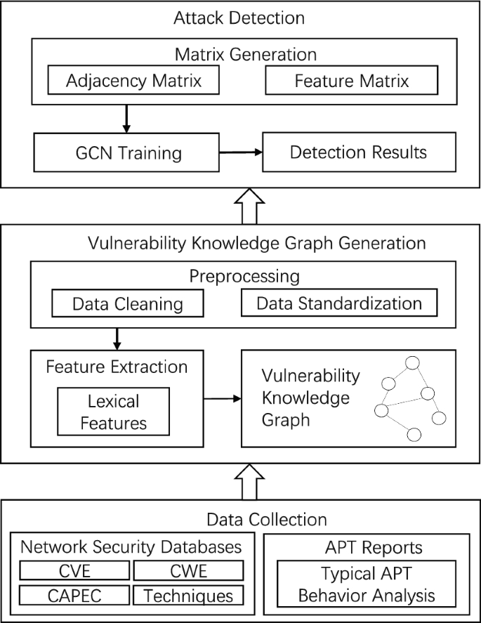
Graph convolutional networks (GCN) is a deep learning model used for graph-structured data, capable of handling complex relationships and network data. APT attacks often utilize multiple vulnerabilities and attack techniques to achieve their objectives, making it possible to model APT attacks as graph-structured data. We use a knowledge graph to conceptualize typical APT organization attacks and the vulnerabilities, techniques, and tools they commonly employ. The GCN model is then used to perform APT attack detection. The overall framework is illustrated in Fig. 1.
This method consists of three main stages: The first stage involves collecting relevant data from network security databases and APT reports and constructing a security knowledge graph. In this graph, typical APT organization attacks are conceptualized along with the vulnerabilities, weaknesses related to vulnerabilities, attack patterns, and attack methods they utilize. These are defined as entities, and their relationships are established. The second stage is knowledge graph feature extraction. In this stage, we first convert the knowledge graph that reflects APT organization vulnerabilities into a homogeneous graph for ease of data input into the GCN model. We then extract features for the CVE (Common Vulnerabilities and Exposures) nodes. The third stage is GCN model design. In this stage, the Graph Convolutional Neural Network algorithm is used to perform information propagation and aggregation on the nodes and edges of the homogeneous graph, ultimately outputting the detection results of whether a node belongs to an APT attack.
Overall framework diagram
Overall framework diagram
4 APT Attack Detection Based on GCN Model
In this section, we provide a detailed implementation process of the proposed method. The first part will introduce the construction of the attack knowledge graph, where entities and relationships are extracted from the descriptions in the crawled network security databases, and then stored using the Neo4j database. The second part will cover APT attack detection using the GCN model. Initially, the heterogeneous attack knowledge graph is transformed into a homogeneous graph, and then feature extraction is performed on this graph. The extracted features will serve as inputs to the GCN model, ultimately achieving APT attack detection.
4.1 Knowledge Graph Construction
This subsection describes constructing a vulnerability knowledge graph by analyzing APT attack reports and security databases. Relevant information, such as APT organization behaviour and CVE vulnerabilities, is extracted from these sources and organized into structured triplets to establish entities and relationships, forming a vulnerability knowledge graph. This graph encompasses vulnerabilities, weaknesses, attack methods, and tactics, utilizing various relationship types to depict their interconnections. This knowledge graph facilitates a comprehensive understanding of the relationships between vulnerabilities and attacks in the software security domain, offering valuable resources and guidance for researching and defending network security.
4.1.1 Collecting Security-Related Data
APT attack reports contain abundant attack context information. Firstly, we perform behavior analysis on typical APT organizations to extract the required information, such as the names of APT organizations and the CVE vulnerabilities, attack methods, and techniques they utilize when launching attacks. Secondly, we organize the collected CVE vulnerabilities and extract the identifier and description of each CVE, CWE (Common Weakness Enumeration), and CAPEC (Common Attack Pattern Enumeration and Classification) from the software security databases (CVE, CWE, CAPEC). Additionally, we establish the interdependencies between them. Lastly, the collected data is stored for subsequent knowledge graph construction.
4.1.2 Entity Modeling
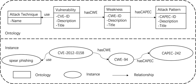
We design a vulnerability knowledge graph by analyzing APT reports, CVE, CWE, CAPEC, and other security information and considering their correlations. Firstly, we extract entities, keywords, and relationships from the unstructured data and represent them in a structured manner using triplets (Entity 1, Relationship, Entity 2). During this process, we only include entities and relationships with relatively high confidence in the knowledge base. The overall structure of the knowledge graph is shown in Fig. 2, consisting of two parts: ontology and instances.
In the ontology design, we divide the graph into four parts: vulnerabilities, weaknesses, attack methods, and attack techniques, each with corresponding attributes. For example, vulnerabilities include CVE-ID, vulnerability description, and title; weaknesses include CWE-ID, weakness description, and title; attack methods include CAPEC-ID, attack method description, and title; attack techniques refer to the specific techniques used in APT attacks, such as spear-phishing attacks and watering hole attacks. Through this structure, we can clearly represent the associations between vulnerabilities and attacks, forming a complete vulnerability knowledge graph.
For instance, APT-C-09 utilizes the CVE-2012-0158 vulnerability for its attack, exploiting CWE-94 as a weakness and adopting the attack method described in CAPEC-242. Ultimately, it implements the attack using techniques such as spear-phishing.
We represent entities and relationships as the primary objects in the security knowledge graph. These entities include core concepts such as CWE (Common Weakness Enumeration) and CAPEC (Common Attack Pattern Enumeration and Classification), as well as instances like CVE (Common Vulnerabilities and Exposures) and the techniques used during attacks. We extract software security entities from CWE, CAPEC, and CVE databases and assign a unique index to each entity, for example, CWE-20, CAPEC-182, and CVE-2018-11882, as shown in Table 2. Each entity is considered a node in the knowledge graph. CWE and CAPEC entities have titles and text descriptions to describe their meanings and characteristics. Each CVE entity has a corresponding text description, providing detailed information about the vulnerability. These pieces of information are integrated into the knowledge graph, allowing us better to understand the associations between security concepts and instances.

Workflow of APT attack detection using GCN

Simplification of the knowledge graph into a homogeneous graph
4.1.3 Relationship Extraction
APT reports describe the vulnerabilities used by APT organizations during attacks, and there are cross-references among security instances in the CVE, CWE, and CAPEC databases. We use these relationships between APT organizations, the vulnerabilities they exploit, and the cross-references as relationships between entities in the knowledge graph, represented in the form of triplets, i.e., <entity, relationship, entity>. The triplets constructed in this study include the following three types of relationships:
<Vulnerability, use, Attack Technique>: Represents the relationship between vulnerabilities and attack techniques, which is a many-to-many relationship.
<Vulnerability, hasCWE, Weakness>: Represents the relationship between vulnerabilities and weaknesses, which is a many-to-many relationship.
<Weakness, hasCAPEC, Attack Pattern>: Represents the relationship between weaknesses and attack patterns, which is a many-to-many relationship.
By constructing such a vulnerability knowledge graph, we can have a more comprehensive understanding of vulnerabilities, weaknesses, and attack patterns in software security. We can also track and analyze the connections between APT organizations and CVE vulnerabilities. This knowledge graph provides valuable resources and references for research and defense work in the security domain, enabling us to address the ever-growing challenges in network security effectively.
4.2 GCN Model Design
In this paper, we use Graph Convolutional Neural Network (GCN) to learn from the constructed vulnerability knowledge graph and perform classification detection of APT attacks based on CVE vulnerabilities and attack context. The security knowledge graph we built contains nodes and edges of different types, each with distinct semantics and attributes. GCN is primarily designed for processing homogeneous graphs, and it cannot be directly applied to the security knowledge graph. Therefore, as shown in Fig. 3, we first need to simplify the security knowledge graph into a homogeneous graph, then extract node features, and finally utilize graph convolutional neural networks for attack detection. The following is a detailed explanation of the algorithm.
4.2.1 Simplification of Heterogeneous Security Knowledge Graph into Homogeneous Graph
In the security knowledge graph G = (V, E) established in this paper, where V is the set of nodes and E is the set of edges, there are 4 types of entities: CVE, CWE, CAPEC, and attack techniques. We aim to detect APT attacks through vulnerability exploitation relationships. CVE nodes are related to the other 3 types of entities. An edge is created if there is a relationship between two CVE nodes. CWE and CAPEC nodes are used as features for the CVE nodes, and the classification of whether the node belongs to an APT attack is considered as the label. As shown in Fig. 4, the heterogeneous security knowledge graph is simplified into a homogeneous graph.
4.2.2 Node Feature Extraction
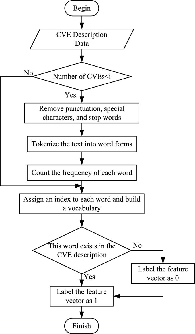
The dataset constructed in this paper is used for studying the APT attack detection task, where each node represents a vulnerability exploited by an APT organization, and the features indicate the presence or absence of certain words. When extracting features, we consider CVE, CWE, and CAPEC. Below, we explain the steps for extracting the feature vectors from the dataset, using CVE as an example. The process is illustrated in Fig. 5:
Flowchart of node feature extraction
Text preprocessing: Download a list of CVE descriptions from the Common Vulnerabilities and Exposures (CVE) database to obtain raw data. Firstly, perform text preprocessing on the CVE descriptions, removing punctuation, stop words and converting the text to lowercase to eliminate case sensitivity. Then, tokenize the preprocessed CVE descriptions, dividing the text into individual words.
Building vocabulary: Traverse all the CVE description data to count the frequency of each word’s occurrence. Construct a vocabulary using high-frequency words and assign a unique index to each word. This vocabulary will be used to represent the feature vectors of the text data.
Feature vector representation: Adopting the bag-of-words model, transform each CVE into a feature vector representation using the constructed vocabulary. Each feature vector dimension corresponds to whether a word from the vocabulary exists in the CVE. If the word exists, the value is set to 1; otherwise, it is set to 0.
CWE and CAPEC node feature extraction: Similar to CVE, when simplifying the knowledge graph into a homogeneous graph, CWE and CAPEC are considered features for each CVE. The CVE’s corresponding CWE and CAPEC are combined to form a feature matrix input.
4.2.3 APT Detection Using Graph Convolutional Neural Network (GCN)
Graph Convolutional Neural Network is a deep learning model designed for graph data, enabling effective feature learning and representation of nodes and edges. We represent the simplified APT homogeneous graph as a node feature matrix X and an adjacency matrix A, which serve as inputs to the GCN model. The feature matrix is an N*D matrix, where N denotes the number of nodes, and D represents the feature dimension of each node. The adjacency matrix is an N*N matrix representing the connectivity between nodes. The propagation rule between layers in GCN is defined as follows:
Among them, \({\tilde{A}}=A+I_N\) is the adjacency matrix with self-loops for the knowledge graph, where \(I_{N}\) is the identity matrix. \({W}^{(\textrm{l})}\) represents the trainable weight, \(\sigma (\cdot )\) is the activation function used in this layer, and \({H}^{(\textrm{l})}\) is the activation matrix for the l-th layer, with \(H^{(l)}=X\) initially. Then, feature propagation (graph convolution operation) is performed by updating node representations using the node feature matrix and the adjacency matrix. In the convolutional layers, we apply the ReLU activation function for feature propagation, enabling the model to learn more complex graph structure features and improve its performance in the prediction task. Finally, applying the softmax function transforms node features into a probability distribution over classes, and the class with the highest probability is chosen as the predicted result. As shown in Fig. 6, this is the graph convolutional neural network model. The model takes the simplified homogeneous graph as input, performs feature extraction through convolutional layers, and outputs the final predicted class for each node. In the graph, each red node sends its feature information transformed to blue neighboring nodes. Each node then aggregates the feature information of its neighboring nodes to fuse local structural information. After aggregating and applying a nonlinear transformation (ReLU), the output becomes the final vector representation and predicted class for the node. Nodes with the same color represent the same category.

Graph convolutional neural network model
Each CVE is treated as a node, and each node has some features, including the CWE weakness corresponding to the CVE vulnerability, the CAPEC attack type, and the APT organization’s attack method. Additionally, each node has a label indicating whether it belongs to an APT attack. The GCN model aggregates the information of neighboring nodes through training to make the detection results more consistent with the true labels. After training is completed, the detection results for APT organizations are output in the test set.
5 Experiment
In this section, we will describe the experiments conducted to evaluate the proposed method. To assess the effectiveness of our approach, we conducted experiments on the constructed dataset. This section will be presented in the following aspects: The first part will introduce the dataset used in the experiments and the evaluation metrics for the model. The second part will describe the implementation of the method, parameter settings, and experimental setup. The third part will present the results of comparative experiments. The fourth part will cover the application experiments of the proposed method.

Model performance comparison of GCN under different parameters. a Performance comparison based on hidden_dim. b Performance comparison based on epoch_num. c Performance comparison based on learning_rate
5.1 Dataset and evaluation metrics
To validate the effectiveness of the proposed detection method, this paper extracted information regarding vulnerability exploitation relationships and attack techniques targeting 12 APT organizations from various threat intelligence sources worldwide, such as CVE, NVD, CNNVD, Qihoo 360, FireEye, and others. Subsequently, CVE vulnerability entities were extracted, and using Xpath, corresponding CWE weakness and CAPEC attack pattern entities’ names and descriptions were crawled from software security databases (CVE, CWE, CAPEC).This process involved collecting software security entity names and detailed descriptions while scraping interdependencies. Finally, the extracted information was integrated to construct the APT attack behavior knowledge graph stored in a Neo4j database. Each entity set comprises CVE, CWE, and CAPEC features, forming a comprehensive dataset. So far, we have collected 2435 labeled attack data and 215 entity relationships from 1350 APT intelligence reports. For the 2435 labeled samples, we performed tenfold cross-validation to mitigate the impact of label imbalance on the experimental results. We used 80% of the samples as the training set, 10% as the validation set, and the remaining 10% of the samples used as the test set.
We employed accuracy, precision, recall, and F1 score as the four key evaluation metrics to assess the model’s performance, which are computed using the number of true positives (TP), false positives (FP), true negatives (TN), and false negatives (FN). The specific formulas are as follows:
Accuracy represents the probability of correct predictions made by the GCN model among all the sample data, reflecting the overall prediction accuracy of the model.
Precision represents the proportion of true attacks among all the samples detected as APT attacks.
Recall represents the proportion of detected attacks among all the true attacks.
The F1 score is calculated using precision and recall and represents their harmonic mean. It can assess the overall performance of the model.
5.2 Parameter Experimentation
We conducted three sets of parameter experiments that affect the model’s performance. Figure 7 illustrates the experimental results under three different parameters. As shown in Fig. 7a, the x-axis represents hidden_dim, which denotes the number of hidden units, a factor influencing the model’s representative capacity. It determines whether the model can learn richer features. With other parameters fixed, as the number of hidden_dim increases from 8 to 16, the model’s accuracy, precision, recall, and F1 score all decrease. The model’s performance gradually improves as we raise it from 16 to 64. When hidden_dim=64, corresponding accuracy, precision, recall, and F1 score all reach their maximum value of 95.8%, indicating the best model performance, further increasing the number of hidden units from 64 to 96 leads to a decrease in model performance. While a slight improvement is observed when increasing the number of hidden units to 128, it remains below the model’s best performance.
As depicted in Fig. 7b, the x-axis represents epoch_num, the number of forward and backward passes of the entire training dataset through the neural network. It affects the model’s training process and results. With other parameters fixed, as we adjust the epoch value to find the optimal training effect, the model’s performance improves as the number of training iterations increases from 50 to 200. However, as we grow the training iterations from 200 to 250, the model’s performance starts to decline. When training iterations go from 250 to 400, the model’s performance improves again, and when epoch=400, the accuracy is 95.1%, precision is 94.9%, recall is 95.2%, and F1 score is 94.9%, all reaching their maximum values. The model’s training performance is at its best. Beyond 400 iterations, the model’s performance remains below the optimal value.

A comparison of attack detection experiments with different sample sizes. a Comparison of accuracy results. b Comparison of precision results. c Comparison of recall results. d Comparison of F1 score results
Figure 7c shows that the x-axis represents learning_rate, which is the main factor determining the gradient descent step size and whether the model can find the global optimum. With other parameters fixed, as we adjust the learning_rate, the model’s performance oscillates slightly when it increases from 0.001 to 0.04. The model’s performance gradually improves as the learning rate increases to 0.06. When learning_rate=0.06, the corresponding accuracy is 95.9%, precision is 95.8%, recall is 95.8%, and F1 score is 95.8%, all reaching their maximum values. The model’s performance is optimal at this point. The model’s performance weakens as we continue to increase the learning rate to 0.09. When rising to 0.1, the model’s performance improves but remains below the optimal value.
In summary, as shown in Table 3, we considered six hyperparameters that affect model performance. When adjusting a specific parameter, other parameters were kept constant. Eventually, we determined that the model achieved its optimal performance with 400 training epochs, 64 hidden units, a learning rate of 0.06, drop_out rate of 0.5, weight decay of 5e\(-\)4, and using the Adam optimizer.
5.3 Comparative Experiments
In this section, we conducted comparative experiments to validate the effectiveness of the graph convolutional neural network (GCN) on the constructed knowledge graph for APT detection. We compared the GCN and graphSAGE models based on the spectral domain. The dataset was divided into five groups with different proportions (20%, 40%, 60%, 80%, and 100%), and the performance of both models was evaluated in terms of accuracy, precision, recall, and F1 score. The experimental results are shown in Fig. 8.
From Fig. 8a, it can be observed that under five different sample sizes, when the data volume is 20%, the accuracy of the GraphSAGE model is 82.8%, while the accuracy of the GCN model is 81.6%. In this scenario, the GraphSAGE model’s detection accuracy is slightly higher than that of the GCN model. For the other data volumes, the accuracy of the GraphSAGE model is 88.2%, 90.1%, 94.1%, and 94.7%, whereas the accuracy of the GCN model is 89.2%, 91.3%, 94.4%, and 95.9%, respectively. It can be seen that the GCN model achieves higher accuracy in scenarios with a more significant number of data entries compared to the GraphSAGE model.From Fig. 8b, when the sample size is small, the precision of the GraphSAGE model is 79.9%, which is lower than the GCN model’s precision of 81.9%. As the sample size increases, the precision of the GCN model becomes 90.4%, 90.7%, 94.6%, and 95.1%, while the GraphSAGE model achieves 88.6%, 89.4%, 94.3%, and 94.6%, respectively. The GCN model consistently outperforms the GraphSAGE model in precision.In Fig. 8c, for the first set of data experiments, the recall of the GraphSAGE model is 79.4%, slightly higher than the GCN model’s recall of 79%. In the subsequent four sets of data experiments, the recall of the GCN model increases to 88%, 92.6%, 94%, and 95.1%, respectively, all of which are higher than the GraphSAGE model’s recall of 87.3%, 90%, 93.7%, and 93.8%.Fig. 8d represents the F1 score of both models under different sample sizes. Similarly, when the sample size is small, the F1 score of the GraphSAGE model is 80.4%, slightly higher than the GCN model’s F1 score of 79.4%. However, as the sample size increases, the GCN model’s F1 score becomes 88.7%, 91.1%, 94.2%, and 95.1%, significantly higher than the GraphSAGE model’s F1 score of 87.7%, 89.6%, 93.9%, and 94.4%.
Although GCN’s performance is slightly lower than GraphSAGE when the sample size is small, as the sample size gradually increases, the GCN model consistently outperforms the GraphSAGE model across all four evaluation metrics. In summary, the GCN model demonstrates better detection performance.
The GCN model used in this study outperforms the GraphSAGE model, especially with larger samples. The main reason is that the GCN model updates the node representations by performing convolutions on the entire graph, allowing it to consider the global structural information of the whole graph more comprehensively. On the other hand, the GraphSAGE model only samples and aggregates a subset of nodes, which can lead to information loss during the sampling process, making it unable to fully utilize the global structural information of the graph. As a result, as the dataset size increases, the GCN model performs better in classification and detection tasks.
The main computational work of this experiment was conducted on a GPU, and the average GPU utilization of the GCN model and the GraphSAGE model was evaluated under the same hardware conditions. The results are shown in Fig. 9. From the figures, it can be observed that on the dataset constructed in this paper, the GPU utilization of the GCN model on different datasets is 8%, 9%, 10%, 10%, and 10%, respectively, with an average utilization of 9.4%. On the other hand, the GraphSAGE model’s GPU utilization is 11%, 11%, 12%, 11%, and 12%, respectively, with an average utilization of 11.4%. Therefore, it can be concluded that the GCN model has a lower average utilization compared to the GraphSAGE model. The main reason is that the GCN model has a simpler structure than the GraphSAGE model. The GCN model mainly consists of graph convolutional layers, while the GraphSAGE model typically includes more complex aggregation functions and sampling strategies. The GCN model has fewer parameters and requires less memory during training and inference, resulting in lower GPU utilization.

Comparison of average GPU utilization for different sample sizes
We compared the two models regarding running time; the results are shown in Fig. 10. It can be observed that the detection time of the GCN model remains relatively stable across different sample data sizes, with times of 2.71s, 2.69s, 2.71s, 2.71s, and 2.72s, within a range of 2.70 ± 0.02s. On the other hand, the GraphSAGE model has shorter detection times when the sample data size is small, with times of 1.87s, 2.08s, and 2.25s, all below 2.70s. As the sample size increases, the detection time for the GraphSAGE model grows to 2.93s and 2.97s, exceeding 2.70s, which is longer than the GCN model’s detection time. This is because the computation in the GCN model is highly parallelized, allowing it to process multiple node features simultaneously, leading to more consistent detection time as the sample size increases. On the other hand, the GraphSAGE model experiences increasing computational complexity per layer with larger sample sizes, resulting in a longer detection time compared to the GCN model.

Comparison of running time for different sample sizes
5.4 Application Experiment
The proposed method in this study associates APT organizations’ attack techniques, exploits CVE vulnerabilities, CWE, and CAPEC, and extracts features using CWE, CAPEC, and attack techniques as attributes for CVE vulnerabilities. The extracted data serves as input for the GCN model, which predicts the labels for each node and edge to determine their relevance to APT attacks. For instance, by inputting CVE-2017-8759, CVE-2014-4114, CVE-2014-6352, CVE-2017-0199, and CVE-2012-0158 into the GCN model for training, the model will predict whether these CVEs are related to APT attacks.
This study predicts the number of true positive and false positive instances for each attack node in the test set to evaluate the model’s detection capability. The results are shown in Table 4. From the overall dataset, 10% of the data was set aside as the test set, comprising 244 data points. Based on the model’s detection results, the data in the test set can be categorized into four scenarios: true positive instances, where the model correctly identified data points related to APT attacks as positive; false positive instances, where the model incorrectly identified data points unrelated to APT attacks as positive; true negative instances, where the model correctly identified data points unrelated to APT attacks as negative; and false negative instances, where the model incorrectly identified data points related to APT attacks as negative. Specifically, there were 98 true positive instances, five false positive instances, 136 true negative instances, and five false negative instances. The detection accuracy reached 95.9%, with precision, recall, and F1-score all at 95.1%.

Comparison between misclassified node and true APT attack. a Misclassified as APT attack CVE-2018-14847. b True APT attack CVE-2018-20250
Based on the detection results, we found a total of 10 nodes that were misclassified. CVE-2018-14847, CVE-2015-6585, CVE-2018-8611, CVE-2016-0189, and CVE-2018-11776 were incorrectly detected as APT attacks. On the other hand, CVE-2020-0688, CVE-2017-11869, CVE-2012-4792, CVE-2017-0143, and CVE-2013-3906 were wrongly classified as non-APT attacks.
The misclassification of these ten nodes is attributed to their possession of similar features. Nodes falsely detected as APT attacks exhibited some similarities in certain features with genuine APT attacks, while nodes falsely detected as non-APT attacks shared feature similarities with fake APT attacks, resulting in false positives. For instance, in Fig. 11a, the vulnerability CVE-2018-14847 is shown with its features, which exploit CWE-22 as a weakness and correspond to the CAPEC-78 attack pattern. These features are also shared with the genuine APT attack CVE-2018-20250, shown in Fig. 11b. However, this similarity is only superficial; in reality, there is no concrete evidence of APT organizations exploiting the CVE-2018-14847 vulnerability for attacks. Therefore, it was erroneously classified as an APT attack during detection. Conversely, some actual APT attacks were incorrectly labeled non-APT attacks because their features resembled the positive instances in the training data but lacked clear evidence of association with APT attacks.
6 Conclusion and Future Work
This paper proposes an APT attack detection method based on Graph Convolutional Neural Networks (GCN) to address the ever-evolving network security threats. We collected threat intelligence reports from various APT organizations, extracted information about the vulnerabilities (CVEs) they exploited during attacks, and used web crawling techniques to obtain entity names and relationships between CVE vulnerabilities, associated weaknesses (CWEs), and attack patterns (CAPECs) from software security databases. We generated triplets of data and constructed an APT attack behavior knowledge graph. The knowledge graph effectively captures rich attack context information and their relationships, thereby improving the accuracy of APT attack detection. The knowledge graph was then transformed into a homogeneous graph, features were extracted from CVE vulnerability nodes, and a Graph Convolutional Neural Network (GCN) model was used to process the graph’s features to detect APT attacks. Four metrics-accuracy, precision, recall, and F1 score-were used on the constructed dataset to evaluate the method’s performance. Furthermore, a comparison was made with the GraphSAGE model. The experimental results demonstrate that the proposed method performs well and can effectively detect APT attacks in real-world scenarios. This study provides an innovative approach to network security by combining the powerful capabilities of knowledge graphs and graph convolutional neural networks, offering robust support for safeguarding information systems and data security.
While this method shows promise in network security, some limitations should be considered. While simplifying the heterogeneous APT attack behavior knowledge graph into a homogeneous graph, some information may be lost, potentially limiting the ability to fully utilize relationships between nodes of different types in some instances. Additionally, the method does not adaptively update the model. Network threat intelligence is an ever-evolving field, with new vulnerabilities, attack methods, and APT organization behaviors emerging continuously. Moreover, threat intelligence data often comes from multiple sources, such as security blogs, vulnerability reports, hacker forums, etc. These data sources require processing and integration before being used for model training and updates. Failure to obtain and update this information in real time may hinder the timely understanding of new threats and the corresponding adjustment of the detection methods.
This paper collected threat intelligence reports from different APT organizations and extracted information related to vulnerability exploits, attack techniques, and the relationships between vulnerabilities and CWE, CAPEC. We constructed a security knowledge graph and proposed an APT attack detection method based on Graph Convolutional Networks (GCN). This method transformed the constructed knowledge graph into a homogeneous graph, extracted features from CVE vulnerability nodes, and then used the GCN model for APT organization classification and detection. To validate the effectiveness of our proposed method, we compared it with the GraphSAGE model. The experimental results demonstrated that our method can effectively detect APT attacks in real-world scenarios.
In future work, we will continue research in the following two aspects:
-
1.
We will extract more threat indicators from APT threat reports, enhance the attack context, reduce the detection of false positives, and consider exploring the effectiveness of heterogeneous graph neural networks on the dataset constructed in this paper for attack detection from a heterogeneous graph perspective.
-
2.
We will propose an adaptive model to address the problem of the model’s inability to adapt to new threat intelligence and attack behaviors.
Data Availability
All the data involved in this article are obtained from public data sets or deleted on the basis of them.
References
Chen, P., Desmet, L., Huygens, C.: A study on advanced persistent threats. In: Communications and Multimedia Security: 15th IFIP TC 6/TC 11 International Conference, CMS 2014, Aveiro, Portugal, September 25-26, 2014. Proceedings 15, pp. 63–72. Springer (2014)
Mohammadzadeh, H., Gharehchopogh, F.S.: A multi-agent system based for solving high-dimensional optimization problems: a case study on email spam detection. Int. J. Commun. Syst. 34(3), e4670 (2021)
Gharehchopogh, F.S.: An improved harris hawks optimization algorithm with multi-strategy for community detection in social network. J. Bionic Eng. 20(3), 1175–1197 (2023)
Virvilis, N., Gritzalis, D.: The big four-what we did wrong in advanced persistent threat detection? In: 2013 International Conference on Availability, Reliability and Security, pp. 248–254. IEEE (2013)
Gharehchopogh, F.S., Ibrikci, T. An improved African vultures optimization algorithm using different fitness functions for multi-level thresholding image segmentation. Multimed Tools Appl (2023). https://doi.org/10.1007/s11042-023-16300-1
Shishavan, S.T., Gharehchopogh, F.S.: An improved cuckoo search optimization algorithm with genetic algorithm for community detection in complex networks. Multimed. Tools Appl. 81(18), 25205–25231 (2022)
Gmz, Y.A.N.G., Zh, T.I.A.N., Wl, D.U.A.N.: The prevent of advanced persistent threat. J. Chem. Pharm. Res. 6(1), 572–576 (2015)
Bridges, R.A., Glass-Vanderlan, T.R., Iannacone, M.D., Vincent, M.S., Chen, Q.: A survey of intrusion detection systems leveraging host data. ACM Comput. Surv. (CSUR) 52(6), 1–35 (2019)
Gharehchopogh, F.S.: Quantum-inspired metaheuristic algorithms: comprehensive survey and classification. Artif. Intell. Rev. 56(6), 5479–5543 (2023)
Singla, A., Bertino, E., Verma, D.: Preparing network intrusion detection deep learning models with minimal data using adversarial domain adaptation. In: Proceedings of the 15th ACM Asia Conference on Computer and Communications Security. Association for Computing Machinery, Taipei, Taiwan, pp. 127–140 (2020)
Han, X., Pasquier, T., Seltzer, M.: Provenance-based intrusion detection: opportunities and challenges. In: 10th USENIX Workshop on the Theory and Practice of Provenance (TaPP 2018). USENIX Association, London (2018)
Jenkinson, G., Carata, L., Bytheway, T., Sohan, R., Watson, R.N.M., Anderson, J., Kidney, B., Strnad, A., Thomas, A., Neville-Neil, G.: Applying provenance in APT monitoring and analysis: practical challenges for scalable, efficient and trustworthy distributed provenance. In: Proceedings of the 9th USENIX Workshop on the Theory and Practice of Provenance (TaPP 2017). USENIX Association, Seattle, WA, p. 16 (2017)
Gharehchopogh, F.S., Ucan, A., Ibrikci, T., Arasteh, B., Isik, G.: Slime mould algorithm: a comprehensive survey of its variants and applications. Arch. Comput. Methods Eng. 30(4), 2683–2723 (2023)
Han, X., Pasquier, T., Bates, A., Mickens, J., Seltzer, M.: Unicorn: runtime provenance-based detector for advanced persistent threats. arXiv preprint arXiv:2001.01525 (2020)
Liu, Y., Zhang, M., Li, D., Jee, K., Li, Z., Wu, Z., Rhee, J., Mittal, P.: Towards a timely causality analysis for enterprise security. In: 2018 Network and Distributed System Security Symposium (NDSS 2018). San Diego (2018)
Hossain, M.N., Milajerdi, S.M., Wang, J., Eshete, B., Gjomemo, R., Sekar R., Stoller, S., Venkatakrishnan, V.N.: \(\{\)SLEUTH\(\}\): Real-time attack scenario reconstruction from \(\{\)COTS\(\}\) audit data. In: 26th USENIX Security Symposium (USENIX Security 17). USENIX Association, Vancouver, BC, pp. 487–504 (2017)
Milajerdi, S.M., Gjomemo, R., Eshete, B., Sekar, R., Venkatakrishnan, V.N.: Holmes: real-time apt detection through correlation of suspicious information flows. In: 2019 IEEE Symposium on Security and Privacy (SP), pp. 1137–1152. IEEE (2019)
Blake E., Andy A., Doug P., Kathryn C., Adam G., Cody B.: Mitre att &ck®: Design and Philosophy. https://attack.mitre.org/docs/ATTACK_Design_and_Philosophy_March_2020.pdf. Accessed 13 Aug 2023
Xiong, C., Zhu, T., Dong, W., Ruan, L., Yang, R., Cheng, Y., Chen, Y., Cheng, S., Chen, X.: Conan: a practical real-time apt detection system with high accuracy and efficiency. IEEE Trans. Dependable Secur. Comput. 19(1), 551–565 (2020)
Barre, M., Gehani, A., Yegneswaran, V.: Mining data provenance to detect advanced persistent threats. In: 11th International Workshop on Theory and Practice of Provenance (TaPP 2019). USENIX Association, Philadelphia, PA (2019)
Berrada, G., Cheney, J., Benabderrahmane, S., Maxwell, W., Mookherjee, H., Theriault, A., Wright, R.: A baseline for unsupervised advanced persistent threat detection in system-level provenance. Future Gener. Comput. Syst. 108, 401–413 (2020)
Xiang, Z., Guo, D., Li, Q.: Detecting mobile advanced persistent threats based on large-scale dns logs. Comput. Secur. 96, 101933 (2020)
Zimba, A., Chen, H., Wang, Z., Chishimba, M.: Modeling and detection of the multi-stages of advanced persistent threats attacks based on semi-supervised learning and complex networks characteristics. Future Gener. Comput. Syst. 106, 501–517 (2020)
Du, M., Li, F., Zheng, G., Srikumar, V.: Deeplog: anomaly detection and diagnosis from system logs through deep learning. In: Proceedings of the 2017 ACM SIGSAC Conference on Computer and Communications Security. Association for Computing Machinery, Dallas, Texas, USA, pp. 1285–1298 (2017)
Shen, Y., Mariconti, E., Vervier, P.A., Stringhini, G.: Tiresias: predicting security events through deep learning. In: Proceedings of the 2018 ACM SIGSAC Conference on Computer and Communications Security. ACM, Toronto, Canada, pp. 592–605 (2018)
Eke, H.N., Petrovski, A., Ahriz, H.: The use of machine learning algorithms for detecting advanced persistent threats. In: Proceedings of the 12th International Conference on Security of Information and Networks. Association for Computing Machinery, Sochi, Russia, pp. 1–8 (2019)
Green alliance technology.: APT organization tracking and governance based on knowledge graph [eb/ol]. https://mp.weixin.qq.com/s/CluHeu1oy7DneBuR0cXZSQ (2020). Accessed 25 June 2023
Najafi, P., Mühle, A., Pünter, W., Cheng, F., Meinel, C.: Malrank: a measure of maliciousness in SIEM-based knowledge graphs. In: Proceedings of the 35th Annual Computer Security Applications Conference. Association for Computing Machinery, San Juan, Puerto Rico, USA, pp. 417–429 (2019)
Acknowledgements
We would like to thanks Jilin Science and Technology Development for funding our work, and the participants and researchers who participated in this study for their contributions.
Funding
This research is funded by Jilin Science and Technology Development Plan Project of China (20230201074GX), and the Jilin Provincial Development and Reform Commission Project (No. 2023C030-3).
Author information
Authors and Affiliations
Contributions
XS developed the idea for the study and wrote the paper. XS, YL and JY performed research. YD and WL collected and analyzed the data. WR and YH reviewed the article.
Corresponding author
Ethics declarations
Conflict of interest
The authors declare no conflict of interest.
Ethics approval and consent to participate
Not applicable.
Consent for publication
Not applicable.
Rights and permissions
Open Access This article is licensed under a Creative Commons Attribution 4.0 International License, which permits use, sharing, adaptation, distribution and reproduction in any medium or format, as long as you give appropriate credit to the original author(s) and the source, provide a link to the Creative Commons licence, and indicate if changes were made. The images or other third party material in this article are included in the article’s Creative Commons licence, unless indicated otherwise in a credit line to the material. If material is not included in the article’s Creative Commons licence and your intended use is not permitted by statutory regulation or exceeds the permitted use, you will need to obtain permission directly from the copyright holder. To view a copy of this licence, visit http://creativecommons.org/licenses/by/4.0/.
About this article

Cite this article
Ren, W., Song, X., Hong, Y. et al. APT Attack Detection Based on Graph Convolutional Neural Networks. Int J Comput Intell Syst 16, 184 (2023). https://doi.org/10.1007/s44196-023-00369-5
Received:
Accepted:
Published:
DOI: https://doi.org/10.1007/s44196-023-00369-5