Variable Selection in the Regularized Simultaneous Component Analysis Method for Multi-Source Data Integration

Abstract

Interdisciplinary research often involves analyzing data obtained from different data sources with respect to the same subjects, objects, or experimental units. For example, global positioning systems (GPS) data have been coupled with travel diary data, resulting in a better understanding of traveling behavior. The GPS data and the travel diary data are very different in nature, and, to analyze the two types of data jointly, one often uses data integration techniques, such as the regularized simultaneous component analysis (regularized SCA) method. Regularized SCA is an extension of the (sparse) principle component analysis model to the cases where at least two data blocks are jointly analyzed, which - in order to reveal the joint and unique sources of variation - heavily relies on proper selection of the set of variables (i.e., component loadings) in the components. Regularized SCA requires a proper variable selection method to either identify the optimal values for tuning parameters or stably select variables. By means of two simulation studies with various noise and sparseness levels in simulated data, we compare six variable selection methods, which are cross-validation (CV) with the “one-standard-error” rule, repeated double CV (rdCV), BIC, Bolasso with CV, stability selection, and index of sparseness (IS) - a lesser known (compared to the first five methods) but computationally efficient method. Results show that IS is the best-performing variable selection method.

Introduction

As a result of recent technological developments, often data from varying types of sources with respect to the same investigation units are gathered and analyzed jointly, which is referred to as multi-source data integration (also known as multi-block data analysis, linked data analysis, and in a broader sense, data fusion¹). In health research, joint analysis combining global positioning systems (GPS) data and self-report travel diary data for the same subjects has been shown to be insightful for understanding people’s traveling behavior, purpose, and immediate environment, providing critical information relevant to health research². In metabolomics, to gain a comprehensive picture of the metabolism in a biological system, researchers have conducted joint analysis on the measures obtained from two different instrumental methods, which are Mass-spectrometry (MS) with gas chromatography (GC/MS) and MS with liquid chromatography (LC/MS)^3,4,5, on the same samples. Multi-source data integration has also been found useful in epigenetics (e.g., joint analysis on genetic information and environmental factors)⁶, in epidemiology (e.g., joint analysis on behavioral data and genetic data)⁷, and in longitudinal and life course studies (e.g., joint analysis on longitudinal survey data and bio-measures)⁸, to name a few.

A popular multi-source data integration methodology often used in social and behavior research, bioinformatics, and analytical chemistry^{9,10,11,12,13,14} is the simultaneous component based data integration method (SCA for short). In essence, SCA is an extension of the well-known principal component analysis (PCA) model¹⁵ to the cases where more than one data block is analyzed. Here, a data block can be, for example, survey data, genetic data, and behavioral data. Under certain constraints imposed on all data blocks, information shared across all data blocks can be extracted and represented by a few components. Thus, by means of dimension reduction, SCA is used to explore and interpret the internal structure that binds all data blocks together. Recent extensions of SCA have greatly improved the flexibility and the usefulness of the method by incorporating regularization such as the Lasso¹⁶ and the Group Lasso¹⁷, resulting in the regularized simultaneous component analysis method (regularized SCA for short)^13,18,19,20. Regularized SCA reveals not only the information shared across all data blocks, which is often referred to as “the common process” or “the joint sources of variation” in the data, but also the information that is unique to certain but not all data blocks, which is referred to as “the specific process” or “the unique variation” underlying the data. Being able to correctly identify and distinguish the common and specific processes is useful and important. For example, Kuppens, Ceulemans, Timmerman, Diener, and Kim-Prieto²¹ pointed out that, in cross-cultural psychology, researchers were often interested in information that was unique to a certain culture (i.e., the specific process), but unfortunately such unique information was usually buried under a vast volume of common traits shared across all cultures (i.e., the common process) and therefore was difficult to be identified. Regularized SCA can be used to identify such unique information. In addition, regularized SCA can handle high-dimensional datasets and, compared to SCA, not only produces sparse results that are much easier to interpret, but also yields consistent estimates²². Such selection of the relevant variables is often needed in practice to hint at what variables to further investigate. As a side note, SCA involves rotating component structure and truncating small loadings to zeros, which may generate misleading results²³. Regularized SCA, however, does not require the rotation or truncation of results. To explain what regularized SCA can offer, we use an application of the method to a three-block parent-child relationship survey dataset documented by Gu and Van Deun¹⁸ as an example.

The parent-child relationship survey dataset consists of three data blocks obtained from a large-scale survey collected from 195 families. For details of this dataset, see Gu and Van Deun¹⁸, and for details of the raw data from which the parent-child relationship survey dataset was retrieved, see Schneider and Waite²⁴. The first data block contains 195 mothers’ opinions with respect to 8 items, including (1) relationship with partners, (2) aggressiveness when arguing with the partner, (3) child’s bright future, (4) activities with the child, (5) feelings about parenting, (6) communication with the child, (7) aggressiveness when communicating with the child, and (8) confidence about oneself. The second data block contains 195 fathers’ opinions regarding the same 8 items. The third data block contains 195 children’s ratings on 7 items, including (1) self confidence/esteem, (2) academic performance, (3) social life and extracurricular activities, (4) importance of friendship, (5) self image, (6) happiness, and (7) confidence about the future. Table 1 shows the descriptive statistics of the dataset. The three data blocks can be jointly analyzed because they share the same investigation units – families. In other words, when the three data matrices are placed side by side (see Fig. 1), each row contains the information of the mother, the father, and the child from the same family. The result of regularized SCA (combined with CV for variable selection) applied to this data set is presented in Table 2, which contains an estimated component loading matrix. The individual loadings contained in Table 2 are interpreted in a similar way as the loadings generated in a PCA analysis, but the power of regularized SCA is that it facilitates the interpretation of joint and specific variation at the block level. The table reveals a few important features of regularized SCA. First, the result is sparse, meaning that redundant information is dropped, facilitating easy interpretations. Second, the method reveals joint and specific processes underlying the three data blocks. For example, Component 1 combines information from all three data blocks, capturing the joint process relevant to the parent-child relationship. Components 2, 3, 4, and 5 reveal specific processes that are unique to the parents (i.e., components 2 and 3), unique to the children (i.e., Component 4), and unique to the fathers (i.e., Component 5). To interpret the components, we use Component 3 as an example. This component suggests that for both the mother and the father, their (good) relationship with the partner, (less) aggressiveness when arguing with the partner, and their (high) self-confidence are positively associated among each other.

Table 1 Descriptive statistics of the parent-child relationship data, obtained from Gu and Van Deun¹⁸.

Figure 1

Joint analysis on multi-source data: Using the parent-child relationship survey dataset as an example.

Table 2 Estimated component loading matrix generated by the regularized SCA method with cross-validation (CV) applied to the parent-child relationship data, obtained from Gu and Van Deun¹⁸.

The parent-child relationship example shows that regularized SCA can be a powerful tool for jointly exploring multiple data sources and discovering interesting internal structures shared among data sources or unique to some but not all data sources. However, to realize its full potential, regularized SCA requires a proper variable selection method for component loadings to ensure that the right structure (i.e., whether components are common or unique) and the right level of sparseness are imposed. Currently, CV with “one-standard-error” rule and stability selection²⁵ have been used together with regularized SCA^19,20. As far as we know, no research has been conducted on the performance of the two variable selection methods: We do not know whether the two methods indeed correctly select important variables (i.e., non-zero component loadings), and if they do, which variable selection method performs better. CV and stability selection are not the only methods for regularized SCA. Other variable selection methods, including information-criterion-based indices and bootstrapping methods, have been proposed for regularized models, such as sparse PCA and regularized regression analysis, but they have not been used for regularized SCA.

In this study, to identify a suitable variable selection method for regularized SCA, we examined the performance of six methods, including CV with “one-standard-error” rule²⁶, stability selection²⁵, repeated double cross-validation (rdCV)²⁷, Index of Sparseness (IS)^28,29,30, Bolasso with CV^31,32,33, and a BIC criterion^34,35. We chose CV with the “one-standard-error” rule, rdCV, IS, and Bolasso, because they had been used successfully in various applications of sparse PCA methods, including early recognition and disease prediction³⁶, schizophrenia research³⁷, epidemics³⁸, cardiac research³⁹, environmental research⁴⁰, and psychometrics⁴¹. We included stability selection because of its popularity in the statistical literature and because it has been used for regularized SCA. We included the BIC criteria by Croux, Filzmoser and Fritz³⁴ and by Guo, James, Levina, Michailidis, and Zhu³⁵ and IS because of their computational efficiency. In addition, we provided an adjusted algorithm of stability selection specifically designed for regularized SCA, and we explained how to use rdCV, IS, Bolasso with CV and the BIC criterion in regularized SCA.

Results

Simulation studies

Data generation

We conducted two simulation studies. In the first simulation study, we evaluated the performance of the variable selection methods when two data blocks were integrated. We considered high dimensional data blocks (i.e., the number of persons smaller than that of variables) and also typical data blocks seen in social sciences (i.e., the number of persons larger than that of variables). The second simulation study extended the first one by integrating four data blocks rather than two data blocks. Both simulation studies followed the same simulation design, and therefore, in the remainder of the section, we outline the design of the first simulation study in details and mention the second simulation study when necessary.

In the first simulation study, the data were generated in five steps.

Step 1: Two data matrices, denoted by X₁ and X₂, were generated. Here we considered three situations:

$$(1)\,{{\bf{X}}}_{1}=\{{x}_{ij}\}\in { {\mathcal R} }^{20\times 40}\,{\rm{and}}\,{{\bf{X}}}_{2}=\{{x}_{ij}\}\in { {\mathcal R} }^{20\times 10},$$

(1)

$$(2)\,{{\bf{X}}}_{1}=\{{x}_{ij}\}\in { {\mathcal R} }^{20\times 120}\,{\rm{and}}\,{{\bf{X}}}_{2}=\{{x}_{ij}\}\in { {\mathcal R} }^{20\times 30},$$

(2)

and

$$(3)\,{{\bf{X}}}_{1}=\{{x}_{ij}\}\in { {\mathcal R} }^{80\times 40}\,{\rm{and}}\,{{\bf{X}}}_{2}=\{{x}_{ij}\}\in { {\mathcal R} }^{80\times 10},$$

(3)

where, for all three situations, ${x}_{ij}\sim i.i.d.N(0,1)$. The choice of how to generate initial structures in this step has little influence on the final results as it only contributes to the true model part; other choices could also have been made, for example using an autoregressive structure on the covariance matrices. Then, the concatenated data matrix with respect to rows, denoted by ${\tilde{{\bf{X}}}}_{C}=[{{\bf{X}}}_{1},{{\bf{X}}}_{2}]$, was of dimension 20 × 50, 20 × 150, and 80 × 50, respectively. In the following, we use the first situation (i.e., Eq. 1) as an example to explain the remaining steps.

Step 2: Using singular value decomposition (SVD), we decomposed ${\tilde{{\bf{X}}}}_{C}$ into U$\Sigma$V. We defined the “true” component score matrix, denoted by T^true, as the matrix containing the three left singular vectors in U corresponding to the three largest singular values. Let $\tilde{\Sigma }$ denote the diagonal matrix containing the three largest singular values, and let $\tilde{{\bf{V}}}$ denote the matrix containing the three right singular vectors corresponding to the three largest singular values. Then, the non-sparse component loading matrix, denoted by ${\tilde{{\bf{P}}}}_{C}$, was ${\tilde{{\bf{P}}}}_{C}=\tilde{{\bf{V}}}\tilde{\Sigma }$.

Step 3: Notice that ${\tilde{{\bf{P}}}}_{C}$ is a 50 × 3 matrix. Let ${\tilde{{\bf{P}}}}_{1}\equiv [{{\bf{p}}}_{1}^{1},{{\bf{p}}}_{2}^{1},{{\bf{p}}}_{3}^{1}]\in { {\mathcal R} }^{40\times 3}$ denote the component loading matrix corresponding to the first block. Let ${\tilde{{\bf{P}}}}_{2}\equiv [{{\bf{p}}}_{1}^{2},{{\bf{p}}}_{2}^{2},{{\bf{p}}}_{3}^{2}]\in { {\mathcal R} }^{10\times 3}$ denote the component loading matrix corresponding to the second block. Thus, ${\tilde{{\bf{P}}}}_{C}\equiv [\begin{array}{c}{\tilde{{\bf{P}}}}_{1}\\ {\tilde{{\bf{P}}}}_{2}\end{array}]$. We assumed that the first component of ${\tilde{{\bf{P}}}}_{C}$ was the common component, representing the common process across both data blocks, and we assumed that remaining two components were distinctive components, representing unique processes, so that ${{\bf{p}}}_{2}^{1}$ in ${\tilde{{\bf{P}}}}_{1}$ and ${{\bf{p}}}_{3}^{2}$ in ${\tilde{{\bf{P}}}}_{2}$ were replaced with 0. As a result, ${\tilde{{\bf{P}}}}_{C}$ became $[\begin{array}{ccc}{{\bf{p}}}_{1}^{1} & {\bf{0}} & {{\bf{p}}}_{3}^{1}\\ {{\bf{p}}}_{1}^{2} & {{\bf{p}}}_{2}^{2} & {\bf{0}}\end{array}]$.

Step 4: We replaced some loadings in ${{\bf{p}}}_{1}^{1}$, ${{\bf{p}}}_{1}^{2}$, ${{\bf{p}}}_{2}^{2}$, and ${{\bf{p}}}_{3}^{1}$ with zeros to make ${{\bf{p}}}_{1}^{1}$, ${{\bf{p}}}_{1}^{2}$, ${{\bf{p}}}_{2}^{2}$, and ${{\bf{p}}}_{3}^{1}$ sparse, and we considered two situations: 30% and 50% of the loadings in ${{\bf{p}}}_{1}^{1}$, ${{\bf{p}}}_{1}^{2}$, ${{\bf{p}}}_{2}^{2}$, and ${{\bf{p}}}_{3}^{1}$ were replaced with zeros. Let ${{\bf{P}}}_{C}^{true}$ denote the concatenated component loading matrix after the sparseness was introduced to $[\begin{array}{ccc}{{\bf{p}}}_{1}^{1} & {\bf{0}} & {{\bf{p}}}_{3}^{1}\\ {{\bf{p}}}_{1}^{2} & {{\bf{p}}}_{2}^{2} & {\bf{0}}\end{array}]$. Note that for notational convenience we used the same symbols for the sparsified loading vectors as previously.

Step 5: We computed ${{\bf{X}}}_{C}^{true}={{\bf{T}}}^{true}{({{\bf{P}}}_{C}^{true})}^{T}$, and added a noise matrix, denoted by E, to ${{\bf{X}}}_{C}^{true}$ to generate the final simulated dataset, denoted by ${{\bf{X}}}_{C}^{generated}$, so that ${{\bf{X}}}_{C}^{generated}={{\bf{X}}}_{C}^{true}+\alpha {\bf{E}}$, where the scalar α is a scaling factor. The cells in E were generated from $N(0,1)$. Note that an implicit assumption of PCA and also SCA is independent and identically distributed noise; other types of noise structure may affect the results. By adjusting α, we were able to control the proportion of noise variance in ${{\bf{X}}}_{C}^{generated}$. We considered two noise levels: 0.5% and 30% of variance in ${{\bf{X}}}_{C}^{generated}$ were attributable to noise.

In summary, the first simulation study included the following design factors:

• Three situations of X₁ and X₂ (i.e., Eqs. 1, 2 and 3).

• Two sparseness levels in ${{\bf{p}}}_{1}^{1}$, ${{\bf{p}}}_{1}^{2}$, ${{\bf{p}}}_{2}^{2}$, and ${{\bf{p}}}_{3}^{1}$: 30% and 50%.

• Two noise levels: 0.5%, and 30%.

  The design factors were fully crossed, resulting in $3\times 2\times 2=12$ design cells. In each design cell, we simulated 20 datasets following the above five steps, and therefore in total 240 datasets were simulated. Then, for each dataset, we conducted the regularized SCA analysis and compared the results generated by the model selection methods, which are CV with “one-standard-error” rule, rdCV, BIC, IS, Bolasso with CV, and stability selection.

  The design of the second simulation study also involved five steps similar to the first simulation, but we made the following changes. In Step 1 of the second simulation study, we considered only one situation:

  $$\begin{array}{rcl}{{\bf{X}}}_{1} & = & \{{x}_{ij}\}\in { {\mathcal R} }^{20\times 120},\\ {{\bf{X}}}_{2} & = & \{{x}_{ij}\}\in { {\mathcal R} }^{20\times 30},\\ {{\bf{X}}}_{3} & = & \{{x}_{ij}\}\in { {\mathcal R} }^{20\times 40},\,{\rm{and}}\\ {{\bf{X}}}_{4} & = & \{{x}_{ij}\}\in { {\mathcal R} }^{20\times 10},\end{array}$$

  (4)

  where ${x}_{ij}\sim i.i.d.N(0,1)$. In Step 3, we inserted 0 in ${\tilde{{\bf{P}}}}_{C}$ such at

  $${\tilde{{\bf{P}}}}_{C}=[\begin{array}{ccc}{{\bf{p}}}_{1}^{1} & {{\bf{p}}}_{2}^{1} & {\bf{0}}\\ {{\bf{p}}}_{1}^{2} & {{\bf{p}}}_{2}^{2} & {{\bf{p}}}_{3}^{2}\\ {{\bf{p}}}_{1}^{3} & {\bf{0}} & {{\bf{p}}}_{3}^{3}\\ {{\bf{p}}}_{1}^{4} & {\bf{0}} & {\bf{0}}\end{array}].$$

  (5)

  In summary, the second simulation study included the following two design factors:

• Two sparseness levels in ${{\bf{p}}}_{1}^{1}$, ${{\bf{p}}}_{2}^{1}$, ${{\bf{p}}}_{1}^{2}$, ${{\bf{p}}}_{2}^{2}$, ${{\bf{p}}}_{3}^{2}$, ${{\bf{p}}}_{1}^{3}$, ${{\bf{p}}}_{3}^{3}$, and ${{\bf{p}}}_{1}^{4}$: 30% and 50%.

• Two noise levels: 0.5%, and 30%.

The design factors were fully crossed, resulting in $2\times 2=4$ design cells. In each design cell, we simulated 20 datasets following the above five steps, and therefore in total 80 datasets were simulated.

Performance measures

To compare the variable selection methods, we used two types of performance measures. The first type concerned the component loading matrix, and the second type concerned the component score matrix. The first type consisted of three performance measures. Let ${\hat{{\bf{P}}}}_{C}$ denote the estimated concatenated component loading matrix. The first performance measure, denoted by PL, was the proportion of non-zero and zero loadings correctly identified in ${\hat{{\bf{P}}}}_{C}$ compared to ${{\bf{P}}}_{C}^{true}$:

$$PL=\tfrac{{\rm{number}}\,{\rm{of}}\,{\rm{correctly}}\,{\rm{selected}}\,{\rm{non}}-{\rm{zero}}\,{\rm{loadings}}+{\rm{number}}\,{\rm{of}}\,{\rm{correctly}}\,{\rm{identified}}\,{\rm{zero}}\,{\rm{loadings}}}{{\rm{total}}\,{\rm{number}}\,{\rm{of}}\,{\rm{loadings}}\,{\rm{in}}\,{{\bf{P}}}_{C}^{true}}\mathrm{}.$$

(6)

Notice that $PL\in [0,1]$. Intuitively, for regularized SCA, the best model selection method should be the one that generating the highest PL among the methods. In addition to PL, we also used PL_{non-0 loadings}, defined as

$$P{L}_{{\rm{non}}-0{\rm{loadings}}}=\tfrac{{\rm{number}}\,{\rm{of}}\,{\rm{correctly}}\,{\rm{selected}}\,{\rm{non}}-{\rm{zero}}\,{\rm{loadings}}}{{\rm{total}}\,{\rm{number}}\,{\rm{of}}\,{\rm{non}}-{\rm{zero}}\,{\rm{loadings}}\,{\rm{in}}\,{{\bf{P}}}_{C}^{true}},$$

(7)

and PL_{0 loadings}, defined as

$$P{L}_{0{\rm{loadings}}}=\tfrac{{\rm{number}}\,{\rm{of}}\,{\rm{correctly}}\,{\rm{identified}}\,{\rm{zero}}\,{\rm{loadings}}}{{\rm{total}}\,{\rm{number}}\,{\rm{of}}\,{\rm{zero}}\,{\rm{loadings}}\,{\rm{in}}\,{{\bf{P}}}_{C}^{true}}\mathrm{}.$$

(8)

We used PL_{non-0 loadings} to evaluate how well a model selection method assisted correctly retaining non-zero loadings and used PL_{0 loadings} to evaluate how well a model selection method assisted correctly identifying zero loadings.

In this study, we focused on the component loading matrix, and we used the variable selection methods to help us identify non-zero and zero loadings, but the component score matrix was also important. Ideally, we would prefer an estimated component score matrix as close as possible to the true component score matrix. Therefore, the second type of performance measure evaluated the degree of similarity between T^true and the estimated component score matrix $\hat{{\bf{T}}}$, quantified by Tucker congruence $\phi$⁴²

$$\phi =\frac{{\rm{vec}}{({{\bf{T}}}^{true})}^{T}{\rm{vec}}(\hat{{\bf{T}}})}{\sqrt{({\rm{vec}}{({{\bf{T}}}^{true})}^{T}{\rm{vec}}({{\bf{T}}}^{true}))({\rm{vec}}{(\hat{{\bf{T}}})}^{T}{\rm{vec}}(\hat{{\bf{T}}}))}}.$$

(9)

Notice that $\phi \in [\,-\,1,1]$. Ideally, a good model selection method for regularized SCA is the one that makes $\phi$ close to 1.

Results

We used the R package RegularizedSCA (version 0.5.5)²⁰ to estimate the regularized SCA model; the R script for replicating the study is included in the supplementary material. All columns in the simulated datasets were mean-centered and scaled to norm one. We used the Group Lasso penalty to identify component structure (i.e., common/distinctive components) and used the Lasso penalty to impose sparseness within a component. For details, please see the Methods section.

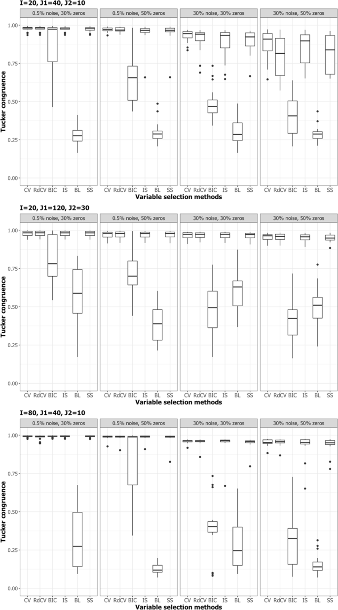
Figures 2, 3, 4 and 5 summarize the results of the first simulation, where two data blocks were integrated. Specifically, Figs. 2, 4 and 5, by means of boxplots, present the performance measures PL (Eq. 6), PL_{non-0 loadings} (Eq. 7), and PL_{0 loadings} (Eq. 8), respectively. Figure 3 presents the boxplots of Tucker congruence measures. For each figure, the upper, middel, and bottom panels correspond to the first, second, and third situations of X₁ and X₂ (i.e., Eqs. 1, 2 and 3), respectively. The reader may notice that most methods (except for BIC and Bolasso) did not differ much in Tucker congruence, and therefore, we focus on discussing PL, PL_{non-0 loadings}, and PL_{0 loadings} and mention Tucker conguence only when necessary.

Figure 2

Integration of two blocks: Proportion of non-zero and zero loadings in ${\hat{{\bf{P}}}}_{C}$ correctly identified (i.e., PL). The upper, middle, and bottom panels correspond to Eqs. 1, 2 and 3, respectively. BL stands for BoLasso with CV. SS stands for stability selection.

Figure 3

Integration of two blocks: Tucker congruences between $\hat{{\bf{T}}}$ and T. The upper, middle, and bottom panels correspond to Eqs. 1, 2 and 3, respectively. BL stands for BoLasso with CV. SS stands for stability selection.

Figure 4

Integration of two blocks: Proportion of non-zero loadings in ${\hat{{\bf{P}}}}_{C}$ correctly selected (i.e., PL_{non-0 loadings}). BL stands for BoLasso with CV. SS stands for stability selection.

Figure 5

Integration of two blocks: Proportion of zero loadings in ${\hat{{\bf{P}}}}_{C}$ correctly identified (i.e., PL_{0 loadings}). BL stands for BoLasso with CV. SS stands for stability selection.

Based on the figures, we concluded the following. First, CV with “one-standard-error” rule and rdCV did not outperform the other methods in most cases in terms of correctly identifying non-zero and zero loadings (see Fig. 2). Figures 4 and 5 show that the two methods tended to retain more non-zero loadings than needed, resulting in high PL_{non-0 loadings} but low PL_{0 loadings}, which is a known feature of CV-based methods⁴³. Second, stability selection was the best-performing method in terms of PL. However, as we have explained in the Methods section, in order for the method to work in the simulation, we assumed that the correct number of non-zero loadings was known a priori, which is unrealistic in practice. Third, IS was the second best-performing method (Fig. 2), witnessed by a balanced, high PL_{non-0 loadings} (Fig. 4) and high PL_{0 loadings} (Fig. 5). Fourth, BIC performed worse than the other methods (except for Bolasso) when the noise level was high (i.e., 30%). Figures 4 and 5 suggest that BIC consistently favored very sparse results, resulting in very high PL_{0 loadings} but low PL_{non-0 loadings}, which in turn lead to low Tucker congruence values (Fig. 3). Finally, Bolasso performed the worst among all the methods in terms of PL and Tucker congruence. This is primarily because the algorithm is very strict: A loading was identified as a non-zero loading only if the loading was estimated to be different from zero in all 50 repetitions (see the Methods section). As a result, the algorithm generated an estimated loading matrix with too many zeros - that is, very high PL_{0 loadings} in Fig. 5 and very low PL_{non-0 loadings} in Fig. 4. Figures 6, 7, 8 and 9 present the results of the second simulation study, where four data blocks were integrated. It may be noted that the four figures are very similar to the Figs. 2, 3, 4 and 5, and therefore, similar conclusions can be made for the second simulation study. For the sake of simplicity, we do not discuss the Figs. 6, 7, 8, and 9.

Figure 6

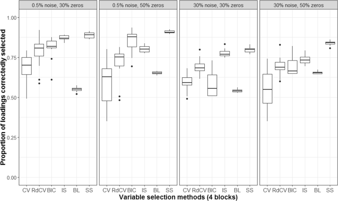
Integration of four blocks: Proportion of non-zero and zero loadings in ${\hat{{\bf{P}}}}_{C}$ correctly identified (i.e., PL). BL stands for BoLasso with CV. SS stands for stability selection.

Figure 7

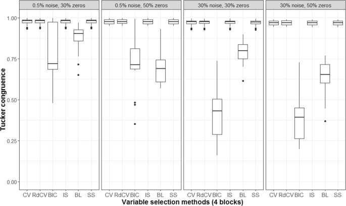
Integration of four blocks: Tucker congruences between $\hat{{\bf{T}}}$ and T. BL stands for BoLasso with CV. SS stands for stability selection.

Figure 8

Integration of four blocks: Proportion of non-zero loadings in ${\hat{{\bf{P}}}}_{C}$ correctly selected (i.e., PL_{non-0 loadings}). BL stands for BoLasso with CV. SS stands for stability selection.

Figure 9

Integration of four blocks: Proportion of zero loadings in ${\hat{{\bf{P}}}}_{C}$ correctly identified (i.e., PL_{0 loadings}). BL stands for BoLasso with CV. SS stands for stability selection.

Based on the two simulation studies, we conclude that, in practice, IS is the best-performing variable selection method for regularized SCA. In addition, more research is needed to improve the stability selection algorithm for regularized SCA so that it will no longer rely on the unrealistic assumption that the correct number of total non-zero loading is known a priori.

Empirical examples

In this section, we present three empirical applications of regularized SCA combined with IS for variable selection. We used the first two empirical examples to explain to the reader how to interpret the estimated component loading matrix generated by regularized SCA together with IS in applied research. The third empirical example is the parent-child relationship data discussed in the Introduction section. We reanalyzed the data by using IS and compared the results with Table 2. We remind the reader that, to evaluate and to interpret the results generated by regularzed SCA, one typically resorts to both the estimated component loading matrix and the estimated component score matrix. In this article, because we focus on variable selection in the component loading matrix, we refrain from discussing the interpretation of the estimated component score matrix in the remainder of this section. Furthemore, for detailed explanation on the use of regularized SCA and the interpretation of the results, we refer to Gu and Van Deun¹⁸.

We used the following setup for IS: 50 Lasso tuning parameter values (equally spaced ranging from 0.0000001 to the smallest value making the entire estimated component loading matrix a zero matrix), and 50 Group Lasso tuning parameter values (equally spaced ranging from 0.0000001 to the smallest value making the entire estimated component loading matrix a zero matrix). All columns in the empirical datasets were mean-centered and scaled to norm one before the regularized SCA analysis was performed.

Joint analysis of the Herring data

In food science, researchers are often interested in the chemical/physical characteristics and the sensory characteristics of a certain food item and analyze the characteristics jointly. An example is the Herring data obtained from a ripening experiment^44,45. In this article, we used part of the original Herring data²⁰, consisting of two datablocks. The first block contained the physical and chemical changes, including pHB, ProteinM, ProteinB, Water, AshM, Fat, TCAIndexM, TCAIndexB, TCAM, and TCAB, of 21 salted herring samples. The meaning of the labels of the physical and chemical changes can be found at http://www.models.life.ku.dk/Ripening_of_Herring. The second block contained the sensory data, including features such as ripened, rawness, malt, stockfish smell, sweetness, salty, spice, softness, toughness, and watery, of the same 21 samples. An interesting research question is whether certain physical and chemical changes are associated with certain sensory characteristics of the herrings. It may be noted that, in this article, we do not discuss how to identify the number of components R (see the Methods section), and for this topic, we refer to Gu and Van Deun¹⁸. A previous study¹⁸ suggested that, for the Herring data, the reasonable number of components R was 4. Therefore, we performed the regularized SCA analysis with IS and $R=4$, and the estimated component loading matrix is presented in Table 3. The table suggests that, for each component, not all variables were important. For example, for Component 1, variables pHB, Water, and AshM from the block of “physical and chemical changes” and variables Ripened, Rawness, Stockfish smell, Sweetness, and Spice from the “sensory” block were important and therefore their loadings were different from zero. To interpret the associations among the variables of Component 1, we primarily look at the signs of the non-zero loadings. For example, for Component 1, variables pHB, Water, Rawness, Sweetness, and Spice were negatively associated with variables AshM, Ripened, Stockfish smell. The remaining three components can be interpreted in the same way.

Table 3 The Herring data: Estimated component loading matrix generated by using regularized SCA with IS.

Joint analysis of metabolomics data

In metabolomics, researchers often use multiple instrumental methods to measure as many metabolites as possible and perform joint analyses by combining the measures on the same metabolites gathered from different instrumental methods⁵. The dataset used in this article contained measures of 28 samples of Escherichia coli (E. coli) obtained from using two measurement methods, which were mass spectrometry with gas chromatograph (GC/MS) and mass spectrometry with liquid chromatography (LC/MS)^3,4. The dataset contained a block of GC/MS data with 144 metabolites and a block of LC/MS data with 44 metabolites. For a detailed description of the dataset, including the experimental design and conditions for obtaining the measures, we refer to Smilde, Van der Werf, Bijlsma, Van der Werff-van der Vat, and Jellema⁵. A previous study¹⁹ suggested that the appropriate number of components R was five. We thus performed the regularized SCA analysis with IS and $R=5$. It may be noted that, in this example, because of the large number of variables, a table of estimated component loading matrix such like Table 3 usually is not practical. Instead, researchers typically use a heatmap so as to get some impression about the sparseness of the loading matrix. Figure 10 presents such a heatmap for the estimated component loading matrix. We found that many loadings in Fig. 10 were very close or equal to zero. As a side note, for this study, researchers typically focus on interpreting the estimated component score matrix instead of the estimated component loading matrix (see, e.g., Van Deun, Wilderjans, van den Berg, Antoniadis, and Van Mechelen⁴⁶).

Figure 10

Joint analysis of metabolomics data: The heatmap for the estimated component loading matrix generated by using IS.

Re-analysis of the parent-child relationship survey data

Table 4 presents the estimated component loading matrix obtained by using IS. The orders of the components were adjusted by using Tucker congruence so that the components in Table 4 are comparable to the components in Table 2 which were generated by using CV¹⁸. The two estimated component loading matrices in Tables 4 and 2 are comparable, and the conclusions based on the two tables are almost the same. For example, for Component 1 of both tables, the last 7 variables from the “Mother” block were positively associated with the variables “child’s bright future”, “feeling about parenting”, “argue with children” from the “Father” block and were also positively associated with the variable “self-confidence/esteem” from the “Child” block.

Table 4 The parent-child relationship data: Estimated component loading matrix generated by using regularized SCA with IS.

Discussion

In this article, we examined six variable selection methods suitable for regularized SCA. The popular CV-based variable selection methods, including CV with “one-standard-error” rule and rdCV, did not outperform other methods. This result may be surprising to many researchers, especially considering that CV seems to be the standard practice when it comes to variable selection. The poor recovery rate of component loadings by using the CV-based methods in the simulations showed that the CV-based methods retained more loadings than needed. Stability selection is a promising method, but at this moment we do not know how to identify an accurate lower bound for the expected non-zero loadings (i.e., Q), making it impossible to tune λ_L. Thus, we advocate the use of IS. It is possible that a hybrid method combining IS and stability selection may perform better than IS. For example, one first uses IS to decide the total number of non-zero loadings and then uses stability selection given the total number of non-zero loadings. Further examination on this idea is needed.

We focused on determining the status of the components (i.e., common/distinctive structure) and their level of sparseness. Another important issue that remains to be fully understood is the selection of the number of components R. Because the goal of this article is to understand variable selection methods for the component loading matrices, the selection of R is beyond the scope of this article. For interested readers, we refer to Bro, Kjeldahl, Smilde, and Kiers⁴⁷, Gu and Van Deun¹⁸, and MÃ¥ge, Smilde, and van der Kloet⁴⁸. We believe that more studies are needed to evaluate the performance of model selection methods for determining R and the performance of variable selection. This may be done sequentially (i.e., first determining R and then, given R, performing variable selection) but also simultaneously (for example, using the index of sparseness to determine R and to perform variable selection at the same time). Finally, we call for studies on comparing the performance of variable selection methods in regularized models. The six variable selection methods studied in this article originated in sparse PCA literature. Therefore, we suspect that stability selection and IS would still outperform the other five methods in the sparse PCA settings. However, we are not aware of any study that compares variable selection methods in sparse PCA.

Admittedly, the six methods studied in this article do not constitute an exhaustive list of all possible variable selection methods for regularized SCA. Other variable selection methods exist, such as the method by Qi, Luo, and Zhao⁴⁹, the information criterion by Chen and Chen⁴³, and the numerical convex hull based method⁵⁰, but they cannot be readily adapted to be used together with regularized SCA. These methods are promising though, and therefore require full attention in separate articles.

Methods

Regularized SCA

Let ${{\bf{X}}}_{k}\in { {\mathcal R} }^{I\times {J}_{k}},(k=1,2,\ldots ,K)$ denote the kth data block with I rows representing subjects, objects, or experimental conditions measured on J_k variables. One may notice that I does not have a subscript k, meaning that all K data blocks are to be analyzed jointly with respect to the same I subjects, objects, or experimental conditions. Each data block may have a different set of variables. Let ${{\bf{X}}}_{C}\in { {\mathcal R} }^{I\times {\sum }_{k}{J}_{k}}$ denote the concatenated data matrix, which is obtained by concatenating X_k s with respect to rows (i.e., ${{\bf{X}}}_{C}\equiv [{{\bf{X}}}_{1},\ldots ,{{\bf{X}}}_{K}]$). Note that I may be much smaller than J_k (i.e., high-dimensional data). Let ${\bf{T}}\in { {\mathcal R} }^{I\times R}$ denote the component score matrix, and let ${{\bf{t}}}_{r},(r=1,\ldots ,R)$ denote the rth column in T. Let ${{\bf{P}}}_{k}\in { {\mathcal R} }^{{J}_{k}\times R}$ denote the component loading matrix for the kth data block, and let ${{\bf{p}}}_{r}^{k},(k=1,\ldots ,K;r=1,\ldots ,R)$ denote the rth column in P_k. Regularized SCA performs data integration by means of solving the following minimization problem,

$$\mathop{{\rm{\min }}}\limits_{{\bf{T}},{{\bf{P}}}_{k}}\,\sum _{k}\,\parallel {{\bf{X}}}_{k}-{\bf{T}}{{\bf{P}}}_{k}^{T}{\parallel }_{2}^{2}+{\lambda }_{L}\,\sum _{k}\,\parallel {{\bf{P}}}_{k}{\parallel }_{1}+{\lambda }_{G}\,\sum _{k}\,\sqrt{{J}_{k}}\parallel {{\bf{P}}}_{k}{\parallel }_{2},$$

(10)

subject to

$${{\bf{T}}}^{T}{\bf{T}}={\bf{I}};{\lambda }_{L},{\lambda }_{G}\ge 0.$$

Regularized SCA performs dimension reduction by imposing a pre-defined number of components, denoted by R ($R\le \,{\rm{\min }}(I,{\Sigma }_{k}{J}_{k})$; for details on deciding R, see Gu and Van Deun¹⁸). ${\sum }_{k}\,\parallel {{\bf{P}}}_{k}{\parallel }_{1}={\sum }_{k}\,{\sum }_{{j}_{k},r}\,|{p}_{{j}_{k}r}|$ is the Lasso penalty¹⁶, and its corresponding tuning parameter is λ_L. ${\sum }_{k}\,\sqrt{{J}_{k}}\,\parallel {{\bf{P}}}_{k}{\parallel }_{2}={\sum }_{k}\,\sqrt{{J}_{k}\,{\sum }_{{j}_{k},r}\,({p}_{{j}_{k}r}^{2})}$ is the Group Lasso penalty¹⁷, and its corresponding tuning parameter is λ_G. Note that if ${\lambda }_{L}=0$ and ${\lambda }_{G}=0$, Eq. 10 reduces to a least squares minimization problem. As a side note, before performing the regularized SCA analysis, all columns in X_k may be mean-centered and scaled to norm one or to ${J}_{k}^{-\mathrm{1/2}}$ in order to give all blocks - even those that contain relatively few variables - equal weight; This procedure is referred to as data pre-processing. However, one may notice that in Eq. 10 the Group Lasso penalty is also weighted by $\sqrt{{J}_{k}}$. Thus, it is likely that, when data are scaled to ${J}_{k}^{-\mathrm{1/2}}$, Eq. 10 would favor data blocks with fewer variables, because the Group Lasso penalty takes $\sqrt{{J}_{k}}$ into account. In addition, because in this study we are interested in identifying the associations between (some) variables across data blocks, penalties are imposed on the component loading matrix^19,46. T is assumed to be the same for all K data blocks, and therefore it serves as a “bridge” linking all data blocks. Information shared among all data blocks or unique to some blocks, such as the loadings in Table 2, is obtained by estimating the component loading matrix ${{\bf{P}}}_{k},(k=1,2,\ldots ,K)$. Assuming T is known, we may further reduce Eq. 10 to

$$\mathop{{\rm{\min }}}\limits_{{{\bf{p}}}_{r}^{k}}\,{\Vert {{\bf{X}}}_{k}^{T}-\mathop{\sum }\limits_{r=1}^{R}\,{{\bf{p}}}_{r}^{k}{{\bf{t}}}_{r}^{T}\Vert }_{2}^{2}+{\lambda }_{L}\,\mathop{\sum }\limits_{r=1}^{R}\,\parallel {{\bf{p}}}_{r}^{k}{\parallel }_{1}+{\lambda }_{G}\sqrt{{J}_{k}}\,\mathop{\sum }\limits_{r=1}^{R}\,\parallel {{\bf{p}}}_{r}^{k}{\parallel }_{2}\mathrm{}.$$

(11)

Let $\hat{{\bf{T}}}$ denote the estimated component score matrix based on Eq. 10, and let ${\hat{{\bf{P}}}}_{k}$ denote the estimated component loading matrix for the kth data block. Further, Let ${\hat{{\bf{P}}}}_{C}\in { {\mathcal R} }^{({\sum }_{k}{J}_{k})\times R}$ denote the concatenated estimated component loading matrix, which is obtained by concatenating all ${\hat{{\bf{P}}}}_{k}\,{\rm{s}}$ with respect to the columns (i.e., ${\hat{{\bf{P}}}}_{C}\equiv {[{\hat{{\bf{P}}}}_{1}^{T},\ldots ,{\hat{{\bf{P}}}}_{K}^{T}]}^{T}$). The algorithm for estimating Eq. 10 requires an alternating procedure where $\hat{{\bf{T}}}$ and ${\hat{{\bf{P}}}}_{C}$ are estimated iteratively. Given ${\hat{{\bf{P}}}}_{C}$, $\hat{{\bf{T}}}$ is obtained by computing $\hat{{\bf{T}}}={\bf{V}}{{\bf{U}}}^{T}$, where U$\Sigma$V^T is the SVD of ${{\bf{P}}}_{C}^{T}{{\bf{X}}}_{C}^{T}$. Given $\hat{{\bf{T}}}$, ${\hat{{\bf{P}}}}_{C}$ is obtained by estimating ${{\bf{p}}}_{r}^{k}(k=1,2,\ldots K;r=1,2,\ldots ,R)$ in Eq. 11 ¹⁸:

$${\hat{{\bf{p}}}}_{r}^{k}={[\frac{1}{2}-\frac{{\lambda }_{G}\sqrt{{J}_{k}}}{2\parallel {\mathscr S}\mathrm{(2}{{\bf{X}}}_{k}^{T}{{\bf{t}}}_{r},{\lambda }_{L}){\parallel }_{2}}]}_{+}{\mathscr S}\mathrm{(2}{{\bf{X}}}_{k}^{T}{{\bf{t}}}_{r},{\lambda }_{L}\mathrm{)}.$$

(12)

In Eq. 12, ${\mathscr S}(\cdot )$ denotes the soft-thresholding operator. The operator [x]₊ is defined as ${[x]}_{+}=x$, if $x > 0$, and ${[x]}_{+}=0$, if $x\le 0$. For details of the estimation procedure, see Algorithm 1 of Gu and Van Deun¹⁸.

Information regarding the position of non-zero/zero loadings in P_C may be known a priori. For example, Bolasso and stability selection procedures, which will be discussed shortly, can be used to identify the position of non-zero/zero loadings. Once the position of non-zero/zero loadings is identified, one uses regularized SCA with ${\lambda }_{L}={\lambda }_{G}=0$ to re-estimate the non-zero loadings in P_C while keeping the zero loadings fixed throughout the estimation procedure. For details of the estimation procedure, see Algorithm 2 of Gu and Van Deun¹⁸.

Variable selection methods

The variable selection methods discussed in this article can be categorized into two groups. The first group, including CV with “one-standard-error” rule, rdCV, BIC criterion, and IS, aims at identifying the optimal λ_L and λ_G for Eq. 10. Once the optimal λ_L and λ_G are obtained, one re-estimates the model by using the optimal λ_L and λ_G. The second group, including the Bolasso with CV and stability selection, aims at identifying the position of non-zero/zero loadings in P_C through repeated sampling. Once the position of non-zero/zero loadings is identified, one re-estimates the non-zero loadings while keeping the zero loadings fixed at zero. In the remainder of this article, we assume that the number of components R is known. To identify R in practice, one may use the Variance Accounted For (VAF) method^9,10 and the PCA-GCA method¹⁴. Both methods are included in the R package “RegularizedSCA”²⁰ (for details on how to use the two methods, see Gu and Van Deun¹⁸). We remind the reader that more research is needed for fully understanding how to identify R.

CV with “one-standard-error” rule

Given a set of λ_L s (consisting of evenly spaced increasing values ranging from a value close to zero, say, 0.000001, to the smallest value making ${\hat{{\bf{P}}}}_{C}={\bf{0}}$), denoted by ${\Lambda }_{L}$, and a set of λ_G s (also consisting of evenly spaced increasing values ranging from a value close to zero to the smallest value making ${\hat{{\bf{P}}}}_{C}={\bf{0}}$), denoted by ${\Lambda }_{G}$, the algorithm searches through a grid of λ_L s and λ_s s (i.e., the Cartesian product of ${\Lambda }_{L}$ and ${\Lambda }_{G}$). For each combination of λ_L and λ_G, denoted by $({\lambda }_{L},{\lambda }_{G})$, the algorithm conducts K-fold CV. Take 10-fold CV for example, 10% of the data cells in X_C are replaced with missing values, and afterwards, missing values in each column are replaced with the mean of that column. The algorithm then computes the mean squared prediction errors (MSPE)⁵¹ for each $({\lambda }_{L},{\lambda }_{G})$. (Suppose a Q-fold CV ($Q=1,\ldots ,q,\ldots Q$) is performed. Let ${{\bf{X}}}_{k}^{(q)}$ denote the data from the kth block for the qth fold. Let ${\hat{{\bf{P}}}}_{k}^{(q)}$ denote the estimated component loading matrix for the kth data block for the qth fold. Let ${\hat{{\bf{T}}}}^{(q)}$ denote the estimated component score matrix for the qth fold. Then MSPE is ${\Sigma }_{q}\,{\Sigma }_{k}\,\parallel {{\bf{X}}}_{k}^{(q)}-{\hat{{\bf{T}}}}^{(q)}{({\hat{{\bf{P}}}}_{k}^{(q)})}^{T}{\parallel }_{2}^{2}/Q$). Let $MSP{E}_{({\lambda }_{L},{\lambda }_{G})}$ denote the MSPE given $({\lambda }_{L},{\lambda }_{G})$. Let $({\lambda }_{L}^{* },{\lambda }_{G}^{* })$ denote the pair that generates the smallest MSPE across all pairs of $({\lambda }_{L},{\lambda }_{G})\,{\rm{s}}$, and let $S{E}_{({\lambda }_{L}^{* },{\lambda }_{G}^{* })}$ denote the standard error of $MSP{E}_{({\lambda }_{L}^{* },{\lambda }_{G}^{* })}$. Applying the “one-standard-error” rule²⁶, the algorithm searches for the optimal pair, denoted by $({\lambda }_{L}^{o},{\lambda }_{G}^{o})$, such that its MSPE, $MSP{E}_{({\lambda }_{L}^{o},{\lambda }_{G}^{o})}$, is closest to but not larger than $MSP{E}_{({\lambda }_{L}^{* },{\lambda }_{G}^{* })}+S{E}_{({\lambda }_{L}^{* },{\lambda }_{G}^{* })}$. As a side note, in the simulation, the algorithm searched the optimal pair whose MSPE was closest to (i.e., could be slightly larger or smaller than) $MSP{E}_{({\lambda }_{L}^{\ast },{\lambda }_{G}^{\ast })}+S{E}_{({\lambda }_{L}^{\ast },{\lambda }_{G}^{\ast })}$. In the simulation, we used 5-fold CV.

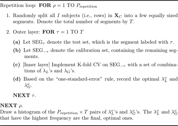
Repeated double cross-validation (rdCV)

The rdCV²⁷, as its name would suggest, is an algorithm that performs double CV repeatedly. Double CV consists of two so-called “layers”, and at each layer a CV is executed. Figure 11 presents a sketch of the algorithm. In the $\rho$th repetition ($\rho =1,\ldots ,{P}_{{\rm{repetition}}}$), the concatenated dataset, X_C, is randomly split into T segments with a (nearly) equal sample size; that is, each segment contains (roughly) the same number of subjects/objects/experimental conditions. The $\tau$th segment, denoted by ${{\rm{SEG}}}_{\tau }$ ($\tau =1,\ldots ,T$), is used as the test set, and the remaining segments constitute the calibration set, denoted by ${{\rm{SEG}}}_{-\tau }$. The algorithm then executes CV with “one-standard-error” rule on ${{\rm{SEG}}}_{-\tau }$ and generates the optimal $({\lambda }_{L}^{o},{\lambda }_{G}^{o})$ for ${{\rm{SEG}}}_{-\tau }$. Thus, in total, ${P}_{{\rm{repetition}}}\times T$ pairs of $({\lambda }_{L}^{o},{\lambda }_{G}^{o})\,{\rm{s}}$ are generated. Note that, in Fig. 11, one may add an extra step after Step (d): In this extra step, one may calculate the MSPE, which provides information for selecting optimal tuning parameters. But Filzmoser, Liebmann, and Varmuza²⁷ suggested that the extra step might be omitted: One may simply use a histogram or a frequency table for the ${P}_{{\rm{repetition}}}\times T$ pairs of ${\lambda }_{L}^{o}\,{\rm{s}}$ and ${\lambda }_{G}^{o}\,{\rm{s}}$ and choose the ${\lambda }_{L}^{o}$ and ${\lambda }_{G}^{o}$ that have been generated most frequently by the algorithm. In the simulation, we let the algorithm choose the most frequently generated ${\lambda }_{L}^{o}$ and ${\lambda }_{G}^{o}$ separately, which was more efficient computationally. In addition, we used 5-fold CV for the inner layer, and for the outer layer, we set the number of segment $T=2$ and the number of repetition ${P}_{{\rm{repetition}}}=50$.

Figure 11

The algorithm of the rdCV.

The BIC criterion

Given a set of λ_L s (consisting of evenly spaced increasing values ranging from a value close to zero, say, 0.000001, to the smallest value making ${\hat{{\bf{P}}}}_{C}={\bf{0}}$), denoted by ${\Lambda }_{L}$, and a set of λ_G s (also consisting of evenly spaced increasing values ranging from a value close to zero to the smallest value making ${\hat{{\bf{P}}}}_{C}={\bf{0}}$), denoted by ${\Lambda }_{G}$, the algorithm searches through a grid of λ_L s and λ_G s (i.e., the Cartesian product of ${\Lambda }_{L}$ and ${\Lambda }_{G}$). For each combination of λ_L and λ_G, denoted by $({\lambda }_{L},{\lambda }_{G})$, the algorithm computes the BIC.

The BIC criterion used in this article is based on two BIC criteria in the sparse PCA literature, one proposed by Croux, Filzmoser, and Fritz³⁴ and the other one by Guo, James, Levina, Michailidis, and Zhu³⁵. We define the variance of the residual matrix if there would be no sparseness in $\hat{{\bf{P}}}$, denoted by V, as $V=\parallel {{\bf{X}}}_{C}-{\hat{{\bf{T}}}}^{(sca)}{({\hat{{\bf{P}}}}_{C}^{(sca)})}^{T}{\parallel }_{2}^{2}$, where ${\hat{{\bf{T}}}}^{(sca)}$ and ${\hat{{\bf{P}}}}_{C}^{(sca)}$ are obtained from the traditional simultaneous component model without Lasso and Group Lasso penalties. We define the variance of the residual matrix given λ_L and λ_G, denoted by $\tilde{V}$, as $\tilde{V}=\parallel {{\bf{X}}}_{C}-\hat{{\bf{T}}}{\hat{{\bf{P}}}}_{C}^{T}{\parallel }_{2}^{2}$, where $\hat{{\bf{T}}}$ and ${\hat{{\bf{P}}}}_{C}$ are obtained from Eq. 10. We define the degrees of freedom given λ_L and λ_G, denoted by $df({\lambda }_{L},{\lambda }_{G})$, as the number of non-zero loadings in ${\hat{{\bf{P}}}}_{C}$. Then the BIC criterion adjusted for regularized SCA, given λ_L and λ_G, based on Croux et al. is

$$BIC({\lambda }_{L},{\lambda }_{G})=\frac{\tilde{V}}{V}+df({\lambda }_{L},{\lambda }_{G})\frac{log(I)}{I},$$

(13)

and the BIC criterion adjusted for the regularized SCA method based on Guo et al. is

$$BIC({\lambda }_{L},{\lambda }_{G})=\frac{I\tilde{V}}{V}+df({\lambda }_{L},{\lambda }_{G})log(I\mathrm{)}.$$

(14)

Notice that the BIC in Eq. 14 is exactly I times the BIC in Eq. 13. Thus, the two methods are in fact equivalent. Then, the optimal tuning parameter values, $({\lambda }_{L}^{o},{\lambda }_{G}^{o})$, are the ones that generate the lowest BIC.

Index of Sparseness (IS)

Given a set of λ_L s (consisting of evenly spaced increasing values ranging from a value close to zero, say, 0.000001, to the smallest value making ${\hat{{\bf{P}}}}_{C}={\bf{0}}$), denoted by ${\Lambda }_{L}$, and a set of λ_G s (also consisting of evenly spaced increasing values ranging from a value close to zero to the smallest value making ${\hat{{\bf{P}}}}_{C}={\bf{0}}$), denoted by ${\Lambda }_{G}$, the algorithm searches through a grid of λ_L s and λ_s s (i.e., the Cartesian product of ${\Lambda }_{L}$ and ${\Lambda }_{G}$). For each combination of λ_L and λ_G, denoted by $({\lambda }_{L},{\lambda }_{G})$, the algorithm computes the IS.

We define the total variance in X_C, denoted by V_o, as ${V}_{o}=\parallel {{\bf{X}}}_{C}{\parallel }_{2}^{2}$. The unadjusted variance assuming no penalty (i.e., ${\lambda }_{L}={\lambda }_{G}=0$), denoted by V_s, is defined as ${V}_{s}=\parallel {\hat{{\bf{T}}}}^{(sca)}{({\hat{{\bf{P}}}}_{C}^{(sca)})}^{T}{\parallel }_{2}^{2}$. Finally, the adjusted variance, denoted by V_a, is defined as ${V}_{a}=\parallel \hat{{\bf{T}}}{\hat{{\bf{P}}}}_{C}^{T}{\parallel }_{2}^{2}$, where $\hat{{\bf{T}}}$ and ${\hat{{\bf{P}}}}_{C}$ are obtained from Eq. 10 (i.e., ${\lambda }_{L}\ne 0$ and ${\lambda }_{G}\ne 0$). Let #_o denote the total number of zero loadings in ${\hat{{\bf{P}}}}_{C}$. Then IS, according to Gajjar, Kulahci, and Palazoglu²⁸ and Trendafilov²⁹, is

$$IS=\frac{{V}_{a}{V}_{s}}{{V}_{o}^{2}}\times \frac{{\#}_{o}}{({\sum }_{k}\,{J}_{k})\times R}.$$

(15)

The optimal tuning parameter values, $({\lambda }_{L}^{o},{\lambda }_{G}^{o})$, are the ones that generate the largest IS.

Bolasso with CV

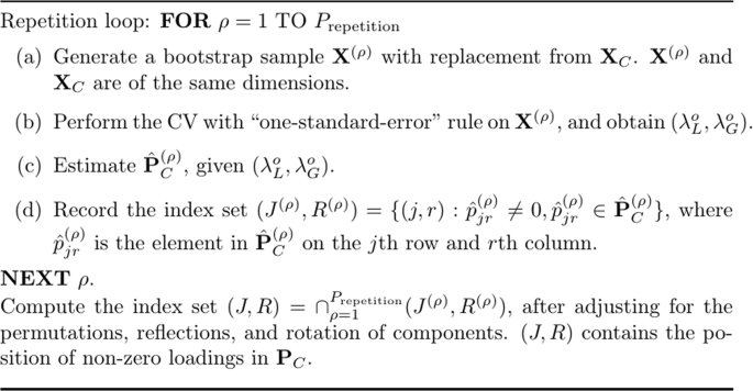
Bolasso, originally proposed by Bach³¹, has been extended to a hybrid procedure combining the original Bolasso with CV^32,33 for stably selecting variables in Lasso regression. Figure 12 presents the algorithm of the Bolasso with CV. In essence, the Bolasso is a bootstrapping procedure. For each bootstrap sample, regularized SCA with K-fold CV is executed, generating the optimal tuning parameters, $({\lambda }_{L}^{o},{\lambda }_{G}^{o})$ based on the “one-standard-error” rule. Afterwards, ${\hat{{\bf{P}}}}_{C}$ is obtained given $({\lambda }_{L}^{o},{\lambda }_{G}^{o})$. Let P_repetition denote the total number of repetitions. Then in total P_repetition ${\hat{{\bf{P}}}}_{C}\,{\rm{s}}$ are generated. The algorithm then compares the P_repetition ${\hat{{\bf{P}}}}_{C}\,{\rm{s}}$, checks which loadings have been estimated to be not zeros for P_repetition times, and records the corresponding index set. As a result, an index set containing the position of non-zero loadings is obtained. Finally, ${\hat{{\bf{P}}}}_{C}$ and $\hat{{\bf{T}}}$ are estimated given the index set. One may notice that because of the invariance of the regularized SCA solution under permutations of components¹⁸, the ${\hat{{\bf{P}}}}_{C}\,{\rm{s}}$ must first be adjusted according to a reference matrix by using the Tucker congruence⁴² (for details, see the R script provided in the supplementary material). As a side note, in the simulation, we used 5-fold CV and let ${P}_{{\rm{repetition}}}=50$.

Figure 12

The algorithm of the Bolasso with CV.

Stability selection

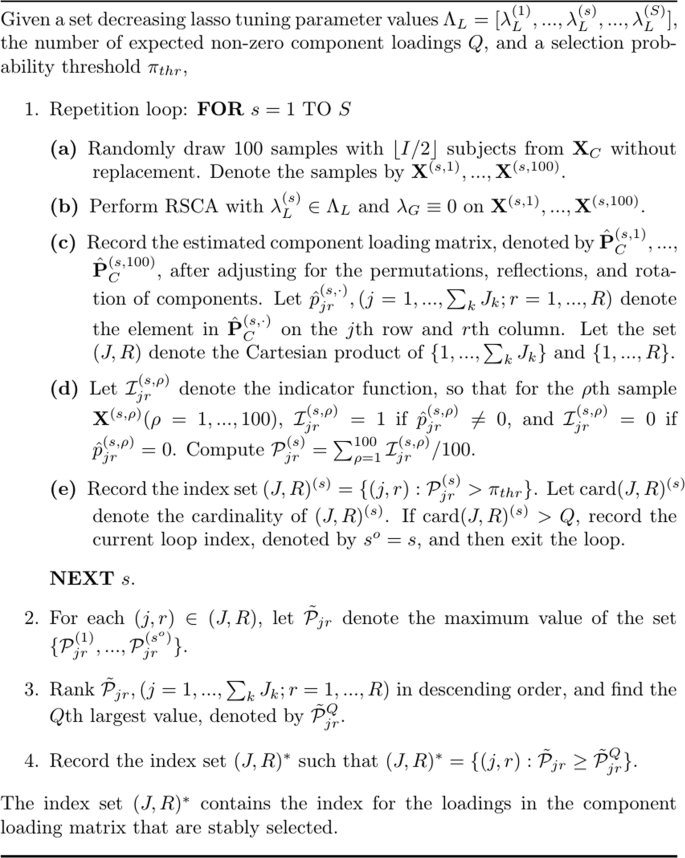
Stability selection²⁵ was demonstrated for variable selection in regression analysis and graphical models based on the Lasso. To use this method for regularized SCA, we have made a few adjustments and present the algorithm in Fig. 13. The algorithm goes through a set of S Lasso tuning parameter values with decreasing order, denoted by ${\Lambda }_{L}=[{\lambda }_{L}^{(1)},{\lambda }_{L}^{(2)},\ldots ,{\lambda }_{L}^{(s)},\ldots ,{\lambda }_{L}^{(S)}]$, $({\lambda }_{L}^{(1)} > {\lambda }_{L}^{(2)} > \cdots > {\lambda }_{L}^{(s)} > \cdots > {\lambda }_{L}^{(S)})$, indexed by $s=1,2,\ldots ,S$. ${\lambda }_{L}^{\mathrm{(1)}}$ is fixed at the minimum value that makes ${\hat{{\bf{P}}}}_{C}\equiv {\bf{0}}$. Given the sth value, ${\lambda }_{L}^{(s)}$, the algorithm works as follows. First, 100 samples with $\lfloor I\mathrm{/2}\rfloor$ subjects (i.e., rows) from X_C are randomly drawn without replacement. For each sample created, regularized SCA with ${\lambda }_{L}^{(s)}$ and ${\lambda }_{G}=0$ is applied. Therefore, the algorithm generates 100 ${\hat{{\bf{P}}}}_{C}\,{\rm{s}}$. Because of the invariance of regularized SCA solution under permutations of components, the ${\hat{{\bf{P}}}}_{C}\,{\rm{s}}$ are adjusted according to a common reference matrix by using the Tucker congruence (for details, see the R script in the supplementary material). Then, the algorithm counts the number of times that the same loading is estimated to be a non-zero loading across the 100 ${\hat{{\bf{P}}}}_{C}\,{\rm{s}}$, which is then divided by 100, resulting in the selection probability for that loading (see Step 1(d) in Fig. 13). As a result, each component loading has a selection probability, which is then compared to a pre-defined selection probability threshold π_thr, and the loadings for which the selection probabilities lower than π_thr are constrained to be zero loadings. The error control theorem proposed by Meinshausen and Bühlmann²⁵ (Theorem 1, p. 7) adjusted for the regularized SCA model is

$$EV\le \frac{1}{2{\pi }_{thr}-1}\times \frac{{Q}^{2}}{R\,{\sum }_{k}\,{J}_{k}},$$

(16)

where EV denotes the expected number of falsely selected variables, Q denotes the expected non-zero loadings, and $R\,{\sum }_{k}\,{J}_{k}$ is the total number of loadings. We notice that, when Gu and Van Deun¹⁹ applied stability selection in their study on regularized SCA, they failed to recognize the problem of Eq. 16: When used for regularized SCA, the lower bound for Q produced by Eq. 16 is not strict enough, making it difficult to tune ${\Lambda }_{L}$. To explain, we use the first simulation study in the Results section as an example and consider the situation of ${{\bf{X}}}_{1}=\{{x}_{ij}\}\in { {\mathcal R} }^{20\times 120}\,{\rm{and}}\,{{\bf{X}}}_{2}=\{{x}_{ij}\}\in { {\mathcal R} }^{20\times 30}$ and 50% of loadings in ${{\bf{p}}}_{1}^{1}$, ${{\bf{p}}}_{1}^{2}$, ${{\bf{p}}}_{2}^{2}$, and ${{\bf{p}}}_{3}^{1}$ are zero loadings. In this case, the total number of non-zero loadings is 150, and the total number of loadings is $R\,{\sum }_{k}\,{J}_{k}=3\times 150=450$. If we use Eq. 16 and let $EV=1$, and ${\pi }_{thr}=0.9$, then $Q\ge 19$, which is much smaller than 150 (i.e, the total number of non-zero loadings). Thus, using Eq. 16 to tune ${\Lambda }_{L}$ is likely to generate a component loading matrix that is too sparse. In this article, the algorithm tunes ${\Lambda }_{L}$ by using the number of expected non-zero component loadings Q, which is assumed known a priori (see Step 1(e) in Fig. 13). Thus, given ${\lambda }_{L}^{(s)}$, if the total number of loadings with selection probability not lower than π_thr is equal to or larger than Q, then the algorithm ignores the remaining Lasso tuning parameter values $[{\lambda }_{L}^{(s+1)},\ldots ,{\lambda }_{L}^{(S)}]$. Assume the algorithm stops at ${\lambda }_{L}^{(s)}$, then for each loading, there are s selection probabilities generated based on $[{\lambda }_{L}^{(1)},\ldots ,{\lambda }_{L}^{(s)}]$. The algorithm records the maximum selection probability across the s selection probabilities for each loading, ranks the loadings in descending order according to their associated maximum selection probabilities, and picks the loadings whose maximum probabilities belong to the first Q maximum probabilities (see steps 2, 3, and 4 in Fig. 13). Finally, the selected loadings are re-estimated, while the remaining loadings are fixed at zero. As a side note, in the simulation, we set ${\pi }_{thr}=0.6$. Also in the simulation, Q was known, which was the total number of non-zero loadings in ${{\bf{P}}}_{C}^{true}$, but this is unrealistic in practice.

Figure 13

The algorithm of stability selection adjusted for regularized SCA.

References

Van Mechelen, I. & Smilde, A. K. A generic linked-mode decomposition model for data fusion. Chemometrics and Intelligent Laboratory Systems 104, 83â94 (2010).
Mavoa, S., Oliver, M., Witten, K. & Badland, H. M. Linking GPS and travel diary data using sequence alignment in a study of childrenâs independent mobility. International Journal of Health Geographics 10, 64 (2011).
Fiehn, O. Metabolomicsâthe link between genotypes and phenotypes. In Functional Genomics, 155â171 (Springer, 2002).
Van Der Werf, M. J., Jellema, R. H. & Hankemeier, T. Microbial metabolomics: Replacing trial-and-error by the unbiased selection and ranking of targets. Journal of Industrial Microbiology and Biotechnology 32, 234â252 (2005).
Smilde, A. K., van der Werf, M. J., Bijlsma, S., van der Werff-van der Vat, B. J. & Jellema, R. H. Fusion of mass spectrometry-based metabolomics data. Analytical Chemistry 77, 6729â6736 (2005).
Meloni, M. Epigenetics for the social sciences: Justice, embodiment, and inheritance in the postgenomic age. New Genetics and Society 34, 125â151 (2015).
Boyd, A. et al. Cohort profile: The âchildren of the 90sââthe index offspring of the Avon Longitudinal Study of Parents and Children. International Journal of Epidemiology 42, 111â127 (2013).
Buck, N. & McFall, S. Understanding society: Design overview. Longitudinal and Life Course Studies 3, 5â17 (2011).
Schouteden, M., Van Deun, K., Pattyn, S. & Van Mechelen, I. SCA with rotation to distinguish common and distinctive information in linked data. Behavior Research Methods 45, 822â833 (2013).
Schouteden, M., Van Deun, K., Wilderjans, T. F. & Van Mechelen, I. Performing DISCO-SCA to search for distinctive and common information in linked data. Behavior Research Methods 46, 576â587 (2014).
van den Berg, R. A. et al. Integrating functional genomics data using maximum likelihood based simultaneous component analysis. BMC Bioinformatics 10, 340 (2009).
Van Deun, K., Smilde, A., Thorrez, L., Kiers, H. & Van Mechelen, I. Identifying common and distinctive processes underlying multiset data. Chemometrics and Intelligent Laboratory Systems 129, 40â51 (2013).
Van Deun, K., Smilde, A. K., van der Werf, M. J., Kiers, H. A. & Van Mechelen, I. A structured overview of simultaneous component based data integration. Bmc Bioinformatics 10, 246 (2009).
Smilde, A. K. et al. Common and distinct components in data fusion. Journal of Chemometrics 31 (2017).
Jolliffe, I. T. Principal component analysis and factor analysis. In Principal Component Analysis, 115â128 (Springer, 1986).
Tibshirani, R. Regression shrinkage and selection via the lasso. Journal of the Royal Statistical Society. Series B (Statistical Methodology) 267â288 (1996).
Yuan, M. & Lin, Y. Model selection and estimation in regression with grouped variables. Journal of the Royal Statistical Society: Series B (Statistical Methodology) 68, 49â67 (2006).
Gu, Z. & Van Deun, K. RegularizedSCA: Regularized simultaneous component analysis of multiblock data in R. Behavior Research Methods 51, 2268â2289 (2019).
Gu, Z. & Van Deun, K. A variable selection method for simultaneous component based data integration. Chemometrics and Intelligent Laboratory Systems 158, 187â199 (2016).
Gu, Z. & Van Deun, K. RegularizedSCA: Regularized Simultaneous Component Based Data Integration, https://CRAN.R-project.org/package=RegularizedSCA, R package version 0.5.4 (2018).
Kuppens, P., Ceulemans, E., Timmerman, M. E., Diener, E. & Kim-Prieto, C. Universal intracultural and intercultural dimensions of the recalled frequency of emotional experience. Journal of Cross-Cultural Psychology 37, 491â515 (2006).
Johnstone, I. M. & Lu, A. Y. On consistency and sparsity for principal components analysis in high dimensions. Journal of the American Statistical Association 104, 682â693 (2009).
Cadima, J. & Jolliffe, I. T. Loading and correlations in the interpretation of principle compenents. Journal of Applied Statistics 22, 203â214 (1995).
Schneider, B. & Waite, L. The 500 family study [1998â2000: United states]. ICPSR04549-v1, https://doi.org/10.3886/ICPSR04549.v1 (2008).
Meinshausen, N. & Bühlmann, P. Stability selection. Journal of the Royal Statistical Society: Series B (Statistical Methodology) 72, 417â473 (2010).
Tibshirani, R., Wainwright, M. & Hastie, T. Statistical learning with sparsity: The lasso and generalizations (Chapman and Hall/CRC, 2015).
Filzmoser, P., Liebmann, B. & Varmuza, K. Repeated double cross validation. Journal of Chemometrics 23, 160â171 (2009).
Gajjar, S., Kulahci, M. & Palazoglu, A. Selection of non-zero loadings in sparse principal component analysis. Chemometrics and Intelligent Laboratory Systems 162, 160â171 (2017).
Trendafilov, N. T. From simple structure to sparse components: a review. Computational Statistics 29, 431â454 (2014).
Zou, H., Hastie, T. & Tibshirani, R. Sparse principal component analysis. Journal of Computational and Graphical Statistics 15, 265â286 (2006).
Bach, F. R. Bolasso: Model consistent lasso estimation through the bootstrap. In Proceedings of the 25th international conference on Machine learning, 33â40 (ACM, 2008).
Hauff, C., Azzopardi, L. & Hiemstra, D. The combination and evaluation of query performance prediction methods. In European Conference on Information Retrieval, 301â312 (Springer, 2009).
Long, Q. & Johnson, B. A. Variable selection in the presence of missing data: Resampling and imputation. Biostatistics 16, 596â610 (2015).
Croux, C., Filzmoser, P. & Fritz, H. Robust sparse principal component analysis. Technometrics 55, 202â214 (2013).
Guo, J., James, G., Levina, E., Michailidis, G. & Zhu, J. Principal component analysis with sparse fused loadings. Journal of Computational and Graphical Statistics 19, 930â946 (2010).
Koutsouleris, N. et al. Early recognition and disease prediction in the at-risk mental states for psychosis using neurocognitive pattern classification. Schizophrenia Bulletin 38, 1200â1215 (2011).
Koutsouleris, N. et al. Accelerated brain aging in schizophrenia and beyond: A neuroanatomical marker of psychiatric disorders. Schizophrenia Bulletin 40, 1140â1153 (2013).
Lampos, V., De Bie, T. & Cristianini, N. Flu detector-tracking epidemics on Twitter. In Joint European conference on machine learning and knowledge discovery in databases, 599â602 (Springer, 2010).
Jin, H. et al. Genome-wide screens for in vivo tinman binding sites identify cardiac enhancers with diverse functional architectures. PLoS Genetics 9, e1003195 (2013).
Gallo, M., Trendafilov, N. T. & Buccianti, A. Sparse PCA and investigation of multi-elements compositional repositories: Theory and applications. Environmental and Ecological Statistics 23, 421â434 (2016).
Trendafilov, N. T., Fontanella, S. & Adachi, K. Sparse exploratory factor analysis. Psychometrika 82, 778â794 (2017).
Abdi, H. Rv coefficient and congruence coefficient. Encyclopedia of Measurement and Statistics 849â853 (2007).
Chen, J. & Chen, Z. Extended bayesian information criteria for model selection with large model spaces. Biometrika 95, 759â771 (2008).
Bro, R., Nielsen, H. H., Stefánsson, G. & SkÃ¥ra, T. A phenomenological study of ripening of salted herring: Assessing homogeneity of data from different countries and laboratories. Journal of Chemometrics 16, 81â88 (2002).
Nielsen, H. H. Salting and ripening of herring: Collection and analysis of research results and industrial experience within the Nordic countries (Nordic Council of Ministers, 1999).
Van Deun, K., Wilderjans, T. F., Van den Berg, R. A., Antoniadis, A. & Van Mechelen, I. A flexible framework for sparse simultaneous component based data integration. BMC Bioinformatics 12, 448 (2011).
Bro, R., Kjeldahl, K., Smilde, A. & Kiers, H. Cross-validation of component models: a critical look at current methods. Analytical and bioanalytical chemistry 390, 1241â1251 (2008).
MÃ¥ge, I., Smilde, A. K. & van der Kloet, F. M. Performance of methods that separate common and distinct variation in multiple data blocks. Journal of Chemometrics 33, e3085 (2019).
Qi, X., Luo, R. & Zhao, H. Sparse principal component analysis by choice of norm. Journal of Multivariate Analysis 114, 127â160 (2013).
Ceulemans, E. & Kiers, H. A. Selecting among three-mode principal component models of different types and complexities: A numerical convex hull based method. British Journal of Mathematical and Statistical Psychology 59, 133â150 (2006).
James, G., Witten, D., Hastie, T. & Tibshirani, R. An introduction to statistical learning, vol. 112 (Springer, 2013).
Acknowledgements
We would like to thank TNO, Quality of Life, Zeist, The Netherlands, for making the metabolomics data available. We thank the anonymous editorial board memberâs and the anonymous reviewersâ valuable suggestions on improving the manuscript. We thank Dr. Davide Vidotto from the department of Methodology and Statistics at Tilburg University for pointing out a mistake in the algorithm of Bolasso with CV in the R script. This research was funded by a personal grant from the Netherlands Organisation for Scientific Research [NWO-VIDI 452.16.012] awarded to Katrijn Van Deun. The funder did not have any additional role in the study design, data collection and analysis, decision to publish, or preparation of the manuscript.
Author information
Authors and Affiliations
Contributions
Z.G. wrote the manuscript, Z.G. and K.V.D. worked out the research idea, Z.G. and N.d.S. conducted the simulation studies and analyzed the results and also the real data examples. All authors revised the manuscript.
Corresponding author
Ethics declarations
Competing interests
The authors declare no competing interests.
Additional information
Publisherâs note Springer Nature remains neutral with regard to jurisdictional claims in published maps and institutional affiliations.
Supplementary information
Rights and permissions
Open Access This article is licensed under a Creative Commons Attribution 4.0 International License, which permits use, sharing, adaptation, distribution and reproduction in any medium or format, as long as you give appropriate credit to the original author(s) and the source, provide a link to the Creative Commons license, and indicate if changes were made. The images or other third party material in this article are included in the articleâs Creative Commons license, unless indicated otherwise in a credit line to the material. If material is not included in the articleâs Creative Commons license and your intended use is not permitted by statutory regulation or exceeds the permitted use, you will need to obtain permission directly from the copyright holder. To view a copy of this license, visit http://creativecommons.org/licenses/by/4.0/.
About this article
Cite this article
Gu, Z., Schipper, N.C.d. & Van Deun, K. Variable Selection in the Regularized Simultaneous Component Analysis Method for Multi-Source Data Integration. Sci Rep 9, 18608 (2019). https://doi.org/10.1038/s41598-019-54673-2
Received:
Accepted:
Published:
DOI: https://doi.org/10.1038/s41598-019-54673-2
This article is cited by
-
Sparsifying the least-squares approach to PCA: comparison of lasso and cardinality constraint
Advances in Data Analysis and Classification (2023)
A Guide for Sparse PCA: Model Comparison and Applications
Psychometrika (2021)
Comments
By submitting a comment you agree to abide by our Terms and Community Guidelines. If you find something abusive or that does not comply with our terms or guidelines please flag it as inappropriate.