


ABSTRACT
We present measurements of the auto- and cross-frequency correlation power spectra of the cosmic (sub)millimeter background at 250, 350, and 500 μm (1200, 860, and 600 GHz) from observations made with the Balloon-borne Large Aperture Submillimeter Telescope (BLAST); and at 1380 and 2030 μm (218 and 148 GHz) from observations made with the Atacama Cosmology Telescope (ACT). The overlapping observations cover 8.6 deg2 in an area relatively free of Galactic dust near the south ecliptic pole. The ACT bands are sensitive to radiation from the cosmic microwave background, to the Sunyaev–Zel'dovich effect from galaxy clusters, and to emission by radio and dusty star-forming galaxies (DSFGs), while the dominant contribution to the BLAST bands is from DSFGs. We confirm and extend the BLAST analysis of clustering with an independent pipeline and also detect correlations between the ACT and BLAST maps at over 25σ significance, which we interpret as a detection of the DSFGs in the ACT maps. In addition to a Poisson component in the cross-frequency power spectra, we detect a clustered signal at 4σ, and using a model for the DSFG evolution and number counts, we successfully fit all of our spectra with a linear clustering model and a bias that depends only on redshift and not on scale. Finally, the data are compared to, and generally agree with, phenomenological models for the DSFG population. This study demonstrates the constraining power of the cross-frequency correlation technique to constrain models for the DSFGs. Similar analyses with more data will impose tight constraints on future models.
Export citation and abstract BibTeX RIS
1. INTRODUCTION
Roughly half of all the light which originated from stars in the extragalactic sky appears as a uniform cosmic infrared background (CIB; Puget et al. 1996; Fixsen et al. 1998). This background peaks in intensity at around 200 μm (Dole et al. 2006) and results from thermal re-radiation of optical and UV starlight by dust grains, meaning that half of all the light emitted by stars is hidden by a veil of dust.
Following its discovery, stacking analyses have statistically resolved most of the CIB shortward of 500 μm into discrete, dusty star-forming galaxies (DSFGs), and to a lesser extent radio galaxies, at z ⩽ 3 (e.g., Dole et al. 2006; Devlin et al. 2009; Marsden et al. 2009; Pascale et al. 2009). Longward of 500 μm, the contribution from radio sources and higher-redshift DSFGs to the CIB increases dramatically with increasing wavelength (e.g., Weiß et al. 2009; Béthermin et al. 2011; Vieira et al. 2010), and as a result, the CIB at these wavelengths has yet to be fully resolved into discrete sources (e.g., Zemcov et al. 2010). Longward of ∼1 mm, in addition to discrete sources, signal from the cosmic microwave background (CMB) becomes visible and dominates the power on angular scales larger than ∼7 arcmin (ℓ ∼ 3000) at λ = 2 mm.
To fully realize the cosmological information encoded in the CMB power spectrum, contributions from discrete sources must be removed. At current millimeter (mm)-wave detection and resolution levels, radio sources are primarily discrete (Poisson) while DSFGs are confusion limited and clustered, so that on large scales power in excess of Poisson resulting from clustered dusty galaxies is non-negligible. For example, at 148 GHz the power spectrum of DSFGs roughly equals the CMB power spectrum at ℓ ≈ 3000. While CMB maps contain signal from multiple contributors, the dominant contributor to submillimeter (submm) maps are dusty galaxies, so that cross-frequency correlations of submm and mm-wave maps provide a unique way of isolating the contribution of DSFGs to CMB maps. However, submm maps of adequate area and depth have until now not existed.
Here we present the measurement of the cross-frequency power spectra of submm and mm-wave maps. We use mm-wave data from the Atacama Cosmology Telescope (ACT; Fowler et al. 2007; Swetz et al. 2010) at 1380 and 2030 μm (218 and 148 GHz), collected during the 2008 observing season, and submm wave data from the Balloon-borne Large Aperture Submillimeter Telescope (BLAST; Pascale et al. 2008; Devlin et al. 2009) at 250, 350, and 500 μm (1200, 860, and 600 GHz), which were collected during its 11 day flight, at ∼40 km altitude, in Antarctica in 2006. We use these to measure the power from DSFGs, both Poisson and clustered. These results will complement those anticipated from the Planck mission (Tauber et al. 2010) by extending to higher resolution in the mm-wave regime.
This paper is organized as follows: In Section 2, we briefly overview the sources of signal in the submm and mm-wave sky, their spectral signatures, and the models we adopt to describe them. In Sections 3 and 4, we describe the data and detail the techniques used to measure the power spectra. We present our results in Section 5 and interpret them in terms of a linear clustering model in Section 6. We discuss and conclude in Sections 7 and 8.
2. THE (SUB)MILLIMETER BACKGROUND
The dominant contribution to the cosmic submm and mm-wave background, referred to hereafter as the CSB, depends strongly on wavelength and angular scale. One map may have contributions from galaxies, CMB, and the Sunyaev–Zel'dovich (SZ) effect simultaneously.
2.1. Power Spectra
The beam-corrected power spectrum of the sky is a superposition, depending on wavelength, of the following terms:
where Cℓ represents the angular power spectrum in multipole space, ℓ, and Nℓ is the noise. Here "cirrus" refers to emission from Galactic dust (Section 2.6), "ff" refers to free–free emission, and "radio" refers to radio sources, GHz-peaked sources and similar objects, whose fluxes increase at longer wavelengths (Section 2.4). It is assumed that diffuse synchrotron emission is negligible. We assume that the various components in Equation (1) are uncorrelated when in reality, correlations among various components likely exist. Such correlations should typically be small and can therefore be reasonably neglected. Furthermore, we define the power from the extragalactic sky as  . The Cffℓ component is assumed to be negligible for the area of the sky we are dealing with. In what follows we report power spectra as both Cℓ and P(kθ), with kθ the angular wavenumber. To convert from multipole ℓ to kθ, or from μK2 to Jy2 sr−1, see Appendix A.
In order to isolate the spectra of one or more contributors to the background requires removal, or adequate modeling, of the unwanted power. Since the contributors have distinct spectral signatures (i.e., their flux densities vary from band to band differently), multi-frequency observations make decomposition of the signal possible. For discrete sources, the ratio of flux densities from band to band is
where  is the "spectral index" and is a function of the rest-frame spectral energy distributions (SEDs) of the sources that make up the galaxy population, and their redshift distributions. Consequently, measurements of the spectral indices can place powerful constraints on source population models (e.g., Marsden et al. 2011; Béthermin et al. 2011).
2.2. CMB
At wavelengths longer than ∼1 mm (ν = 350 GHz) the CMB dominates the power spectrum on scales greater than ∼8'. Multiple peaks in the spectrum have been measured most recently by Brown et al. (2009), Friedman et al. (2009), Reichardt et al. (2009a, 2009b), Sayers et al. (2009), Lueker et al. (2010), Sharp et al. (2010), Fowler et al. (2010), Das et al. (2011), and Nolta et al. (2009). Secondary anisotropies include CMB lensing, which acts to smooth out the peaks and add excess power to the damping tail; and the SZ effect, which distorts the primordial CMB signal.
In the present analysis, the CMB power in ACT maps, which dominates on large scales, does not correlate with signal in the BLAST maps; however, it does act to increase the noise on those scales (see Appendix B).
2.3. Dusty Star-forming Galaxies
DSFGs, as their name implies, are galaxies undergoing vigorous star formation, much of which is optically obscured by dust. They have average flux densities of 5 mJy (at 250 μm; Marsden et al. 2009), star formation rates (SFRs) of ∼100–200 M☉ yr−1 (Pascale et al. 2009; Moncelsi et al. 2011), number densities of ∼2 × 10⁻⁴ Mpc−3 (e.g., van Dokkum et al. 2009), and typically lie at redshifts 0–4, with the peak in the distribution at z ∼ 2 (Amblard et al. 2010). They are distinguished from "submillimeter galaxies" (SMGs) discovered by SCUBA (Smail et al. 1997; Hughes et al. 1998; Eales et al. 1999), which are 10 times less abundant (Coppin et al. 2006), lie at slightly higher redshifts (Chapman et al. 2005), have SFR ∼ 1000 M☉ yr−1, and are thought to be triggered largely by major mergers (Engel et al. 2010). They are of course related: SMGs comprise the extreme, high-redshift end of the DSFG population.
The dust in DSFGs absorbs starlight and re-emits it in the IR/submm, with an SED phenomenologically well approximated by a modified blackbody,

where B(ν) is the Planck function and β is the emissivity index (whose value typically spans 1.5–2; e.g., Draine & Lee 1984). The SED of a typical DSFG with temperature ∼30 K and β = 2 (Chapin et al. 2011) peaks at rest-frame λ ≃ 100 μm (which redshifts into the submm at z ∼ 1–10). A property of this shape is that with increasing redshifts, observations in the (sub)mm bands continue to sample at a rest-frame wavelength close to the peak of the SED, so that even though sources become more distant, their apparent flux remains roughly constant. This so-called negative K-correction makes observations at longer wavelengths more sensitive to higher-redshift sources (Blain et al. 2003). As a result, sources at z ≳ 1 have a significant impact on the power spectrum at (sub)mm bands.
The cross-frequency power spectrum between bands 1 and 2 arising from unclustered sources is related to the number counts—i.e., the surface density N as a function of flux density S—as follows:
where dN/dSΔS is the number of sources per unit solid angle in a flux bin of width ΔS, at frequency bands 1 and 2, and Scut is the flux density at which the counts are truncated. When the slope of the counts is steeper than −3, the power diverges at low flux densities, and the power spectrum is dominated by the contribution to the background from faint sources. In the case of DSFGs, the strong evolution of the source counts with redshift results in a steep slope at the faint end (Devlin et al. 2009), so that after masking local sources (with Scut ≲ 500 mJy) the DSFG component of the CIB at λ > 250 μm is dominated by faint sources and remains finite.
Since DSFGs are spatially correlated (Viero et al. 2009, hereafter V09), their power spectrum has both Poisson and clustered components:

The measured strength of the clustered component is such that it dominates over the Poisson on scales ≳ 3' (V09; Marsden et al. 2009; Hall et al. 2010; Dunkley et al. 2011; Shirokoff et al. 2011), with the exact value depending on frequency and flux cut. How the strengths of the Poisson and clustering terms scale with wavelength, and if they evolve together or independently, remain open questions.
We compare to the models of Béthermin et al. (2011, hereafter B11) and Marsden et al. (2011, hereafter M11) for DSFGs at the BLAST and ACT wavebands. These are phenomenological models which are specifically tailored to constrain the evolution of the rest-frame far-infrared peak of galaxies at redshifts up to z ∼ 4.5. The models use similar Monte Carlo fitting methods but differ in a few ways, e.g., the B11 model is fit using data (predominantly number counts) from a very wide range of IR wavelengths (15 μm to 1.1 mm) while M11 uses only data that constrains the evolution of the far-IR (FIR) peak and was not fit to any observations with λ < 70 μm. B11 also divides galaxies into two distinct populations based on luminosity and attempts to account for the strong lensing of high-redshift galaxies; M11 does neither of the above.
2.4. Radio Galaxies
Synchrotron, and to a lesser extent free–free emission, dominates the SEDs of radio galaxies at rest-frame λ ≳ 1 mm. Thus radio galaxies become an increasingly important contribution to the CSB at wavelengths greater than ∼1.5 mm (ν ≲ 200 GHz). Their number counts are relatively shallow (e.g., de Zotti et al. 2010), meaning that their contribution to the power spectrum is dominated by the brighter sources, resulting in primarily Poisson noise.
While radio sources are a significant source of power at 2030 and 1380 μm, they do not feature prominently in the cross-frequency correlation of ACT and BLAST maps, so we do not include them in our models for the cross-spectra. They do, however, contribute to the uncertainties in the cross-power spectrum, as is described in Appendix B.
2.5. SZ
The SZ effect (Sunyaev & Zeldovich 1972) is the distortion of the microwave background due to interaction of CMB photons with free electrons in clusters, and consists of two main physical mechanisms, referred to as "thermal " and "kinetic." The thermal term (tSZ) is the inverse Compton scattering of CMB photons as they pass through the intracluster medium in galaxy clusters. The result is that the intensity of the CMB spectrum longward of 1380 μm (218 GHz) decreases (i.e., a decrement), while that shortward of 1380 μm increases (i.e., an increment), and 1380 μm is the null for the non-relativistic case. The kinetic term (kSZ) is the Doppler shift of scattered CMB photons by the bulk motion of galaxy clusters. The strength of the signal is proportional to the product of the free electron density and line-of-sight velocity.
2.6. Cirrus
On large angular scales, a significant source of fluctuation power is emission from Galactic cirrus. Although the south ecliptic pole (SEP) field is among the least contaminated by cirrus in the sky (Imean = 1.16 MJy sr−1), contributions from Galactic cirrus must still be accounted for.
The power spectrum of Galactic cirrus has been shown in many studies to exhibit power-law behavior. Its amplitude varies over the sky, but its slope is always between −2.6 and −3 (e.g., Gautier et al. 1992; Boulanger et al. 1996; Miville-Deschênes et al. 2007; Bracco et al. 2011). In the FIR/submm bands, the SED of Galactic cirrus is well described by a modified blackbody (Equation (3)), with T = 17.5 K and β ∼ 1.9, peaking at λ ∼ 150 μm (V09; Bracco et al. 2011). As a result, bands closest to the SED peak (in our case 250 μm) are most susceptible to contamination.
As one moves far from the SED peak, Finkbeiner et al. (1999) show that the modified blackbody approximation breaks down, and a multi-component fit is a much better description of the data. Therefore, for this analysis we measure the power spectrum at 100 μm for the SEP region and adopt model 8 of Finkbeiner et al. (1999) to estimate the amplitude of the power in our bands.
3. INSTRUMENTS AND OBSERVATIONS
3.1. ACT
ACT is a 6 m off-axis Gregorian telescope (Fowler et al. 2007) situated at an elevation of 5190 m on Cerro Toco in the Atacama desert in northern Chile. ACT has three frequency bands centered at 148 GHz (2.0 mm), 218 GHz (1.4 mm), and 277 GHz (1.1 mm) with angular resolutions of roughly 1 4, 10, and 09, respectively. The high altitude site in the arid desert is excellent for mm observations due to low precipitable water vapor and stability of the atmosphere. The tropical location of ACT permits observations of both the northern and southern celestial hemispheres. Further details on the instrument are presented in Swetz et al. (2010), Fowler et al. (2010), and references therein.26 The ACT maps used in this paper are made from data taken during the 2008 observing season (at 148 GHz and 218 GHz, or 2030 and 1380 μm, respectively) and are identical to the maps used in Hajian et al. (2010) and Das et al. (2011). The beam full widths at half-maxima (FWHM) are 14 and 10 at 148 GHz and 218 GHz, respectively (Hincks et al. 2010). The maps have mean 1σ sensitivities which vary slightly across the maps, ranging from 2.4–3.5 mJy beam−1 (median ≈2.7 mJy beam−1) and 3.2–5.4 mJy beam−1 (median ≈3.7 mJy beam−1), at 148 GHz and 218 GHz, respectively (Das et al. 2011). The map projection used is cylindrical equal area (CEA) with square pixels, 05 on a side. The ACT data set is divided into four equal subsets in time, such that the four independent maps generated from these subsets cover the same area and have similar depths. We call these "sub-maps." As described in Hajian et al. (2010), the ACT maps are directly calibrated to the Wilkinson Microwave Anisotropy Probe (WMAP). This results in a 2% fractional temperature uncertainty for the 148 GHz maps. The calibration error for the 218 GHz maps is 7%.
Because the ACT maps have poorly measured modes on the largest angular scales, we filter them using a high-pass filter Fc(ℓ) in Fourier space. The high-pass filter is a smooth sine-squared function in Fourier space given by

where x(ℓ) = (π/2)(ℓ − ℓmin)/(ℓmax − ℓmin) and Θ is the Heaviside function. We choose ℓmin = 100 and ℓmax = 500. Moreover, the large-scale CMB in the ACT maps acts as noise in cross-correlations with the BLAST maps, since the CMB is absent in the latter. If not filtered, the large angular scale and CMB noise terms contaminate the real-space cross-frequency correlations described in Section 3.4. Therefore we use a filter with ℓmax = 2200 when dealing with real-space cross-frequency correlations. The analyzed power spectra are corrected for this filter as well as for the effects of the beam and pixel window functions.
3.2. BLAST
BLAST flew for 11 days from Antarctica in 2006 December. As a pathfinder for the SPIRE instrument (Griffin et al. 2003), it made observations at 250, 350, and 500 μm, of a number of targets, both Galactic and extragalactic. Its 1.8 m underilluminated primary resulted in beams with FWHM of 36'', 45'', and 60''. For a detailed description of the instrument see Pascale et al. (2008) and Truch et al. (2009).27
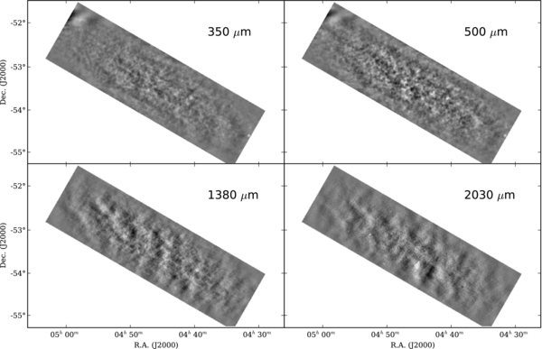
Among the fields BLAST observed is an 8.6 deg2 rectangle near the SEP—chosen because it is a relatively low-cirrus window through the Galaxy (see Section 2.6)—whose corners lie at [(5h02m, −52°50'); (4h57m, −51°35'); (4h25m, −54°19'); (4h30m, −55°41')] (see Figure 1). Further studies of the SEP field, including BLAST catalogs and 24 μm maps, can be found in Valiante et al. (2010) and Scott et al. (2010). The maps have mean 1σ sensitivities of 36.7, 27.2, and 19.1 mJy beam−1 at 250, 350, and 500 μm, respectively. Furthermore, confusion noise, due to multiple point sources occupying a single beam element, is estimated to be 7.6, 6.0, and 4.4 mJy beam−1 at 250, 350, and 500 μm, respectively. The 1σ uncertainty on the absolute calibration is accurate to 9.5%, 8.7%, and 9.2% at 250, 350, and 500 μm, respectively.
Figure 1. Four of the maps used in this analysis: the BLAST maps at 350 and 500 μm (top) and the ACT data at 1380 and 2030 μm for the same region (bottom). Long wavelength modes in the ACT maps have been removed using the high-pass filter described in Equation (6). All maps are multiplied by a taper as discussed in the text. Download figure:
The BLAST time-ordered data are divided into four sets— covering the same region of the sky to the same depth—from which we make four unique sub-maps. The number of subsets is chosen to maximize the number of maps that can be made while maintaining uniformity in hits and providing as much cross-linking as possible. The maps are made with the iterative map maker SANEPIC (Patanchon et al. 2009) resulting in a transfer function of unity on the scales of interest. These sub-maps are unique to this study and are publicly available at http://blastexperiment.info/results.php.
Due to poor cross-linking, however, large-scale noise, resembling waves in the map, is present. This noise is easily dealt with by filtering in Fourier space, as described in Section 4. Maps are made in tangent-plane projection, with 10'' pixels. In order to cross-correlate with ACT, BLAST maps are re-binned to ACT resolution and reprojected to CEA projection using Montage.28 We confirm the alignment by analyzing the real-space cross-frequency correlation, described in detail in Section 3.4.
3.3. IRIS
To estimate the contribution from Galactic cirrus we use three IRIS (reprocessed IRAS; Miville-Deschênes & Lagache 2005) HCON29 maps at 100 μm. These maps are consistent with the Finkbeiner et al. (1999, hereafter FDS) maps used for estimating the contribution from Galactic cirrus in Das et al. (2011), but they are at a higher resolution. Since we are most interested in large-scale modes, the power spectrum is measured for a 30 deg2 field surrounding the SEP (see Figure 2).
3.4. Comparing Data Sets: Testing Alignment with Real-space Cross-correlations
We test that the maps are properly aligned by inspecting their real-space cross-frequency correlations. This is done by inverse Fourier transforming the two-dimensional cross-frequency correlation of the Fourier components of the maps:
where ℓ is a vector in Fourier space, and a(ℓ) and b(ℓ) are the ACT and BLAST maps in Fourier space, respectively. Fc(ℓ) denotes the high-pass filtering in Fourier space described in Equation (6). The resulting measured real-space cross-frequency correlation function M encodes the celestial correlation function between the bands as

where ⊗ denotes a convolution in real space, B(x) is the effective beam between the two maps, and n(x) is the noise. Perfectly aligned maps would result in a two-dimensional cross-frequency correlation function whose peak lies at x = 0. The shape of Ma × b(x) depends on the correlation length of the field, the high-pass filtering, and the beams. (See Hajian et al. 2010 for a comparison between measurements of a real-space cross-frequency correlation function and simulations for a related example.) As illustrated in Figure 3, we measure a cross-correlation with a peak at x = 0 (zero lag), indicating that the maps are correlated and properly aligned.
4. MEASURING AUTO- AND CROSS-FREQUENCY POWER SPECTRA
4.1. Power Spectrum Method
We use a flat-sky approximation for computing the power spectra, which are measured from Fourier transforms of the maps. We use three distinct types of power spectra: the BLAST auto-band spectra, the BLAST cross-band spectra, and the ACT/BLAST cross-band spectra.
The maps can be represented as

where  is the sky temperature signal, N is the noise, B is the instrument beam and we use ⊗ to represent a convolution in real space. Both the ACT and BLAST maps are made with unbiased iterative map makers, whose transfer functions are approximately unity on the angular scales of interest in this study, and can thus be safely neglected.
All power spectra, both auto- and cross-frequency spectra, are computed using cross-correlations of sub-maps (described in Sections 3.1 and 3.2), the advantage being that the noise between sub-maps is uncorrelated and thus averages to zero in the cross-spectra. A cross-power spectrum computed this way provides an unbiased estimator of the true underlying power spectrum. The power spectrum methods used in this paper closely follow those used for cross-correlating ACT and WMAP in Hajian et al. (2010).
BLAST × BLAST power spectra are computed using the average of the six cross-correlations between the four BLAST sub-maps (in each band), such that
where α and β index the four sub-maps. The reason for six cross-correlations, rather than nine, is that cross-frequency cross-correlations of sub-maps made from the same scans are not used, in order to avoid introducing correlated noise or other systematic effects.
Since the noise in all ACT and BLAST sub-maps is uncorrelated, we co-add the sub-maps for each frequency before computing the ACT×BLAST power spectra. The ACT × BLAST power spectra are computed from these maps. This is identical to cross-correlating all ACT sub-maps with all BLAST sub-maps and averaging them.
Several components contribute to the cross-spectrum uncertainties. An analytic approach to computing the uncertainties is described in Appendix B.
4.2. Weights and Masks
We adopt techniques developed in Hajian et al. (2010) in order to isolate and remove or downweight instrumental and systematic noise. This is done in two stages, in real space and in Fourier space, before reducing the two-dimensional spectrum into the familiar one-dimensional angular power spectrum binned in radius (ℓ). The ACT × BLAST cross-spectra are limited by the area of the BLAST maps, which are 1 5 × 57 rectangles (∼8.6 deg2), rotated by approximately 30°, and with noisy edges (see Figure 1). To apodize the sharp edges in the maps, we use the first Slepian taper (properties of which are described in Das et al. 2009) defined on the BLAST region. The gradual fall-off of this taper at the edges reduces the mode–mode coupling in the measured power spectrum. Any residual mode coupling caused by this weighting is corrected in the end by deconvolving the window function (i.e., the power spectrum of the taper function) from the measured power spectrum using the algorithm described in Hivon et al. (2002) and Das et al. (2009). Large-scale noisy modes are best treated in Fourier space. The statistical isotropy of the universe leads to an isotropic two-dimensional power spectrum from extragalactic sources, on average. Anisotropic power in two-dimensional Fourier space is caused by noise and is optimally dealt with using inverse noise weighting, which involves dividing the two-dimensional spectra by our best estimate of the two-dimensional noise power spectrum for each map. At each frequency, the noise model is computed from the difference between the average two-dimensional auto- and cross-spectra for each pair of maps, as described in Hajian et al. (2010). For every cross-correlation, noise weights are computed from the inverse of the square root of the product of the two noise power spectra corresponding to the two frequency bands. The weights are whitened by dividing by their angular averaged value with a fine binning. Using simulations we confirm that this weighting does not bias the signal power spectrum. Anisotropic, large-scale noise is evident at the center of the two-dimensional power spectrum, as shown in Figure 4. Noise weighting downweights the noisy vertical stripe that passes through the origin, which is predominantly due to large-scale unconstrained modes in the map (see also Fowler et al. 2010). To further ensure that our results are not contaminated by this stripe, we mask a vertical band spanning |ℓx| < 500 before averaging the two-dimensional power spectra in annuli. Our results are invariant under further widening of this mask. In order to be consistent with the V09 analysis, we make a mask to remove all point sources that have a flux greater than 0.5 Jy in the BLAST 250 μm map (six sources). We use that mask for computing BLAST power spectra only. For cross-correlations of ACT and BLAST, we instead mask just the brightest source in BLAST maps, which happens to be a local spiral galaxy. We confirm that masking more point sources does not have an effect on the cross-spectra. We also mask the known radio galaxies (Marriage et al. 2011) in the ACT 2030 μm map to reduce the uncertainties in the cross-spectra (see Appendix B).
4.3. Estimating Galactic Cirrus Emission
IRIS maps at 100 μm contain three potential sources of power—diffuse Galactic emission (or cirrus), as well as the Poisson and clustered terms of the DSFG power spectra. Cirrus dominates the power spectrum on angular scales ℓ ≳ 800, but varies depending on the observed patch of sky. The Poisson level is highly sensitive to the adopted flux cut. Thus, in order to detect the signal from clustering, both the cirrus and Poisson noise must be sufficiently low. This is achieved by observing in a clean patch of sky, and cutting bright point sources. We realize these criteria by considering only the SEP (Imean = 1.16 MJy sr−1) and by cutting sources with Scut > 1 Jy.
Miville-Deschênes et al. (2007) show that the power spectrum of Galactic cirrus can be approximated by a power law,
where kθ is the angular wavenumber in inverse arcminutes and P0 is the power spectrum value at k0 ≡ 0.01 arcmin−1.
We are only concerned with the modes that affect our measurement, and since the cirrus power spectrum falls steeply with increasing kθ, we focus our attention on the larger-scale modes. In order to probe these modes with maximum resolution in Fourier space, we measure the cirrus component of a ∼30 deg2 region of the IRIS data surrounding the SEP field as indicated in Figure 2. We filter the IRIS maps using the high-pass filter of Equation (6). The power spectrum is computed from the mean of the three cross-spectra from the three HCON maps (using one taper at resolution 1; see Das et al. 2009 for details).
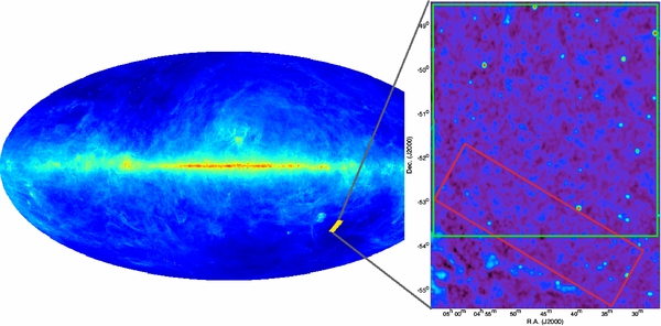
Figure 2. Full-sky IRIS map at 100 μm scaled logarithmically. The red outline represents the BLAST field in CEA projection, which is used for cross-frequency correlating with the ACT maps. The region clearly has low dust contamination. The bigger square area outlined by a green line shows the 30 deg2 region used for estimating the IRIS power spectrum. This map is filtered with the high-pass filter of Equation (6).
Download figure:
Standard image High-resolution image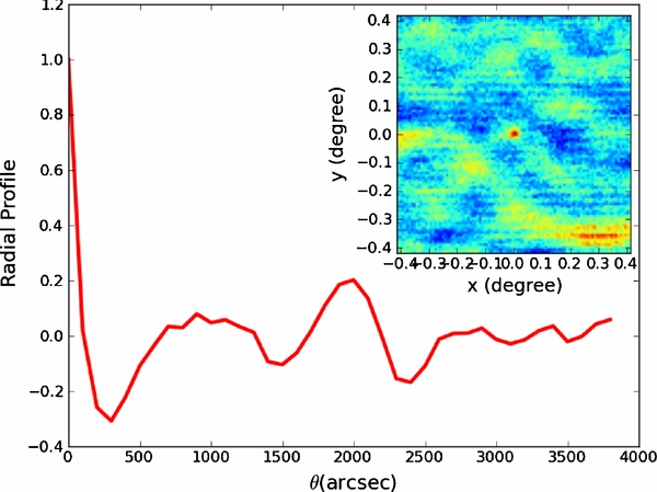
Figure 3. Radial profile of the two-dimensional cross-frequency correlation function between the ACT 1380 μm band and the BLAST 500 μm is plotted with arbitrary normalization, with an image of the two-dimensional function inset. The function has a clear peak at zero lag. This shows the two data sets are aligned and there is a correlated signal in the maps. Large-scale fluctuations (at θ ≳ 500'') are caused by the atmospheric noise and the CMB. The maps are filtered by the high-pass filter of Equation (6) with ℓmin = 100 and ℓmax = 2200 to remove longer wavelength noise.
Download figure:
Standard image High-resolution image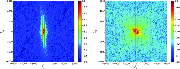
Figure 4. Estimated two-dimensional noise power spectrum for (a) 250 μm and (b) 1380 μm. The noise model is computed from the difference of the auto- and cross-power spectra. Noise due to scan-synchronous signals and other large-scale correlations, which contaminates the signal in the central region, is down-weighted with this weight map in Fourier space, and then further filtered with a vertical mask spanning |ℓx| < 500. The weights are normalized by the maximum value of the noise power spectrum and are plotted in a log scale.
Download figure:
Standard image High-resolution imageWe attempt to fit the data in two ways, where in both cases we fix the slope of the cirrus power spectrum at α = −2.7 (adopting the properties of region 5 of Bracco et al. 2011, whose mean flux density most resembles the SEP). The first is a two-parameter fit, where the free variables are the Poisson level and the amplitude of the cirrus power. For this we find P0 = (0.47 ± 0.06) × 106 Jy2 sr−1 and χ2 = 21.9 (dof = 29). The measured power spectrum is shown in Figure 5. The power spectrum uncertainties are calculated in a manner analogous to that described in Appendix B.
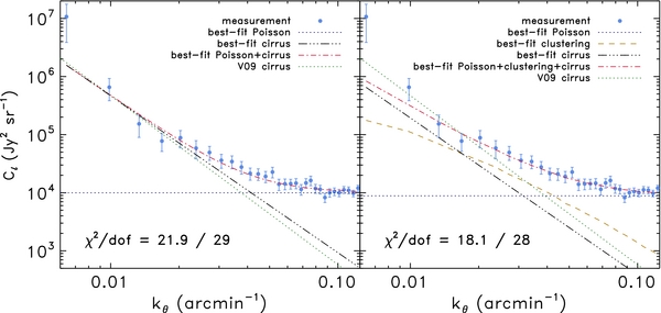
Figure 5. Power spectrum of the 30 deg2 region surrounding the SEP from IRIS 100 μm maps. A three-component fit (left panel), including a clustering term (dashed yellow line) provides a better description of the measured power spectrum than fitting just Poisson and cirrus alone (right panel), but the difference is not statistically significant.
Download figure:
Standard image High-resolution imageThe second fitting procedure uses a three-parameter fit in which the free variables are the Poisson level, cirrus amplitude, and clustering amplitude of the DSFGs. The shape of the clustering component is simply that of a linear dark matter spectrum. In this case we find cirrus values P0 = (0.19 ± 0.15) × 106 Jy2 sr−1 and a clustering amplitude of ∼720 Jy2 sr−1 at ℓ = 3000, with χ2 = 18.1(dof = 28).
The two approaches estimate consistent Poisson levels, but the fit with a clustered component appears to describe the data better than without, with Δχ2 = 3.8. While not yet statistically significant, future studies with Photodetector Array Camera and Spectrometer at 100 μm (Poglitsch et al. 2010) should be able to measure the clustered signal to high significance. The cirrus power spectrum is assumed to continue to smaller angular scales and is estimated at the ACT and BLAST bands using the average dust emission color  , which is estimated using model 8 of Finkbeiner et al. (1999).
5. POWER SPECTRUM RESULTS
The BLAST auto-band and cross-band power spectra and BLAST × ACT cross-frequency power spectra are shown in Figure 6. Raw data are shown as squares, while cirrus subtracted points are shown as crosses with error bars. The Galactic cirrus spectra, interpolated to our bands as described in Section 2.6, are shown as dashed lines in the bottom left corner of each panel (when strong enough to appear at all). Cirrus appears to have a nearly negligible effect on the power in most bands, with only a marginal contribution in the 250 μm auto-spectrum. Note, the cirrus contribution in V09 to the BLAST bands was extrapolated from 100 μm incorrectly; however, properly accounting for cirrus ultimately has little impact on the final result. The cirrus-corrected data are given in Table 2. We describe the models and the fits to these data in Section 6.
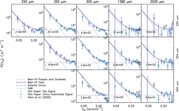
Figure 6. BLAST × BLAST (250–500 μm) and ACT × BLAST (1380–2030 μm) power spectra in P(kθ) with 1σ error bars. Squares and crosses are the data before and after cirrus removal. Red exes and red horizontal dotted lines are published power spectra and Poisson noise levels from V09. The dotted blue lines, which are horizontal and which are falling with kθ, are the best-fit Poisson and clustering terms, respectively. The departure from Poisson is the evidence for clustering of DSFGs. Note that the vertical scale is different for each panel. The error bars are described in Appendix B.
Download figure:
Standard image High-resolution imageThe figure shows a clear cross-correlation between ACT and BLAST. There is both a significantly correlated Poisson term (horizontal line) and a clear clustering term (rising to low kθ). This is the main result of this paper: that the unresolved BLAST background made up of DSFGs is intimately related to the ACT unresolved background. The signal is clearest in the ACT 1380 μm correlation with BLAST 500 and 350 μm, and less significant in the ACT 1380 and 2030 μm correlation with BLAST 250 μm. Additionally, the figure confirms the V09 BLAST power spectrum analysis and extends it to include the cross-frequency correlation between BLAST bands.
Not shown in Figure 6 are predictions for the cross-correlation of the SZ increment and decrement, nor are predictions for the cross-correlations of the SZ decrement and DSFGs shown. Both of these signals would appear as anti-correlated at the ACT 2030 μm band and would act to decrease the total sky signal. The former, using templates of Battaglia et al. (2010), was predicted to be negligibly small; and while at some level the latter should exist, we have not yet identified a clear signature.
6. LINEAR CLUSTERING MODEL
In this section, we estimate the DSFG Poisson power levels and fit the clustered component using a simple linear model similar to that of V09 and Hall et al. (2010). We assume that the clustered component of the DSFG power spectrum, PDSFG, is related to the linear dark matter power spectrum, PDM, through a single bias parameter b(z):

so that the angular power spectrum, P(kθ), of DSFGs can be written as
(Bond et al. 1991; Tegmark et al. 2002), where x(z) is the comoving distance, dVc/dz = x2dx/dz is the comoving volume element, and dI/dz is the contribution to the intensity from sources at redshift z.
We adopt dI/dz from the source model of B11. Figure 7 shows plots of dI/dz from the model at 250 and 2030 μm for 10 randomly chosen realizations provided by the B11 distribution.30 We adopt the concordance model, a flat ΛCDM cosmology with ΩM = 0.274, ΩΛ = 0.726, H0 = 70.5 km s−1 Mpc−1, and σ8 = 0.81 (Hinshaw et al. 2009).
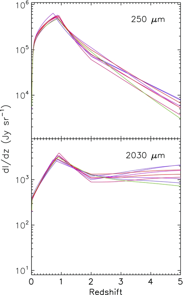
Figure 7. Redshift distributions of intensity, dI/dz, at 250 and 2030 μm for 10 arbitrarily chosen realizations of the B11 source model. In this model the emission peaks around z = 1 for the whole range of wavelengths covered by ACT and BLAST, but there are significant contributions to the IR flux from z ≳ 2 at mm wavelengths.
Download figure:
Standard image High-resolution imageThe linear dark matter power spectrum is calculated as PDM(k) = P0(k)D2(z)T2(k), where P0(kθ) is the primordial power spectrum, T(kθ) is the matter transfer function with fitting function given in Eisenstein & Hu (1998), and D(z) is the linear density growth function. For simplicity we treat the magnitude of the Poisson component of each of the 12 power spectra as free parameters.
We note that our model does not account for nonlinear, one-halo clustered power. Though likely present, the data are not sufficiently constraining given that the Poisson power dominates over or is degenerate with the one-halo term over the angular scales to which we are sensitive.
6.1. Estimating the Bias
In principle the bias, b, is a function of scale and redshift, as well as environmental factors such as the host halo mass of DSFGs. Here we adopt a simple redshift-dependent bias of the form (Bond et al. 1991; Hui & Parfrey 2008)
where D(z) is the linear growth function and b0 is an initial bias at some formation redshift, z0. This parameterization assumes that DSFGs are members of a single population, which formed at the same epoch (z0) and under the same conditions.
Our parameter space consists of the 12 Poisson levels plus b0 and z0. However, just as the Poisson contribution is a sum over the galaxy distribution, weighted by the square of the fluxes (Equation (4)), the average bias is a sum weighted linearly by the flux (e.g., Bond 1993). Thus, in any physical model for the star-forming objects and their bias, the two terms would be correlated in a model-dependent way; we therefore choose to adopt an independent bias for simplicity. Decoupling the Poisson level and the clustered component means the interpretation of our derived b is not straightforward. We find that moderate changes in z0 (in the range 6 < z0 < 10) have virtually no effect on the quality of the fit or best-fit b(z), and also find that b0 and z0 are almost degenerate, and so we fix z0 = 8. We explore the remaining 13-parameter space using a Markov Chain Monte Carlo (MCMC) method with uniform priors on each parameter. We fit the ACT×BLAST data in the range ℓ = 950 (kθ = 0.04 arcmin−1) and ℓ = 9000.
We find a best-fit b0 = 18.2+2.3− 1.7 with χ2 = 107 for 101 degrees of freedom. This corresponds to b(z = 1) = 5.0+0.6− 0.4 and b(z = 2) = 6.8+0.8− 0.5. This Poisson-plus-clustering model is preferred to the null case with no ACT×BLAST correlation at over 25σ. The best-fit clustering and Poisson levels are reported in Table 1 and are plotted as blue dotted lines in Figures 6 and 9.
Table 1. Best-fit CPoissonℓ and Cclusteringℓ(ℓ = 3000), Including Predictions for the Clustered Power at the Three Effective ACT Bands
| Cℓ | Band (μm) | 250 | 350 | 500 | 1380 | 2030 |
|---|---|---|---|---|---|---|
| 250 | (1.1 ± 0.1) × 107 | (9.1 ± 0.6) × 104 | (3.1 ± 0.3) × 103 | (1. ± 0.4) × 101 | (5.9 ± 1.9) × 100 | |
| Cpℓ(μK2) | 350 | ... | (1.1 ± 0.1) × 103 | (3.4 ± 0.3) × 101 | (1.8 ± 0.3) × 10−1 | (1.0 ± 0.2) × 10−1 |
| 500 | ... | ... | (1.8 ± 0.1) × 100 | (7.3 ± 1.0) × 10−3 | (4.6 ± 0.7) × 10−3 | |
| 250 | (6.1 ± 1.1) × 106 | (7.3 ± 1.1) × 104 | (3.6 ± 0.3) × 103 | (9.3 ± 1.1) × 100 | (3.6 ± 0.4) × 100 | |
| 350 | ... | (8.7 ± 1.2) × 102 | (4.4 ± 0.6) × 101 | (1.2 ± 0.2) × 10−1 | (4.7 ± 0.7) × 10−2 | |
| Ccℓ = 3000(μK2) | 500 | ... | ... | (2.1 ± 0.3) × 100 | (6.9 ± 1.1) × 10−3 | (2.6 ± 0.4) × 10−3 |
| 1380 | ... | ... | ... | (3.4 ± 1.0) × 10−5 | (1.2 ± 0.3) × 10−5 | |
| 2030 | ... | ... | ... | ... | (4.4 ± 1.2) × 10−6 | |
Notes. Predictions for the Poisson power at ACT bands are not provided as the Poisson terms are treated as free parameters when obtaining the best fit (see Section 6).
Download table as: ASCIITypeset image
Table 2. Measured ℓ2Cℓ/2π (μK2) from Figure 9 (Blue Crosses)
| ℓ | 950 | 1750 | 2650 | 3550 | 4450 | 5350 | 6250 | 7150 | 8050 |
|---|---|---|---|---|---|---|---|---|---|
| 250 × 250 | (1.2 ± 0.6) × 1013 | (1.4 ± 0.8) × 1013 | (2.6 ± 0.5) × 1013 | (2.7 ± 0.8) × 1013 | (3.5 ± 0.7) × 1013 | (6.8 ± 1.0) × 1013 | (8.7 ± 1.1) × 1013 | (1.2 ± 0.1) × 1014 | (1.1 ± 0.2) × 1014 |
| 250 × 350 | (1.2 ± 0.5) × 1011 | (2.0 ± 0.4) × 1011 | (2.0 ± 0.4) × 1011 | (2.6 ± 0.5) × 1011 | (3.0 ± 0.6) × 1011 | (5.0 ± 0.7) × 1011 | (7.6 ± 0.9) × 1011 | (9.1 ± 1.0) × 1011 | (9.2 ± 1.3) × 1011 |
| 250 × 500 | (4.3 ± 2.0) × 109 | (5.7 ± 1.9) × 109 | (8.3 ± 1.7) × 109 | (1.2 ± 0.3) × 1010 | (1.3 ± 0.2) × 1010 | (2.1 ± 0.3) × 1010 | (2.7 ± 0.3) × 1010 | (3.0 ± 0.4) × 1010 | (2.6 ± 0.5) × 1010 |
| 250 × 1380 | ... | (3.2 ± 3.4) × 107 | (1.4 ± 2.8) × 107 | (4.7 ± 3.7) × 107 | (7.4 ± 3.0) × 107 | (9.7 ± 2.8) × 107 | (1.1 ± 0.5) × 108 | (1.5 ± 0.5) × 108 | (1.3 ± 0.7) × 108 |
| 250 × 2018 | ... | (2.2 ± 2.2) × 107 | (2.9 ± 19.4) × 106 | (8.2 ± 8.9) × 106 | (3.6 ± 1.3) × 107 | (6.3 ± 1.9) × 107 | (1.3 ± 2.8) × 107 | (5.4 ± 4.0) × 107 | (5.0 ± 6.4) × 107 |
| 350 × 350 | (1.4 ± 0.8) × 109 | (2.2 ± 0.7) × 109 | (3.4 ± 0.5) × 109 | (4.1 ± 0.5) × 109 | (4.2 ± 1.4) × 109 | (6.4 ± 0.8) × 109 | (5.8 ± 1.0) × 109 | (9.5 ± 1.2) × 109 | (1.3 ± 0.1) × 1010 |
| 350 × 500 | (6.5 ± 2.8) × 107 | (9.7 ± 2.8) × 107 | (9.5 ± 1.8) × 107 | (1.4 ± 0.2) × 108 | (1.6 ± 0.4) × 108 | (2.2 ± 0.3) × 108 | (2.6 ± 0.4) × 108 | (3.6 ± 0.6) × 108 | (3.1 ± 0.4) × 108 |
| 350 × 1380 | ... | (4.7 ± 2.0) × 105 | (3.6 ± 1.5) × 105 | (6.3 ± 2.6) × 105 | (6.1 ± 1.7) × 105 | (1.2 ± 0.2) × 106 | (1.5 ± 0.3) × 106 | (2.4 ± 0.4) × 106 | (2.3 ± 0.7) × 106 |
| 350 × 2018 | ... | (2.3 ± 1.2) × 105 | (7.5 ± 9.6) × 104 | (2.5 ± 0.9) × 105 | (3.5 ± 1.0) × 105 | (7.5 ± 1.4) × 105 | (3.9 ± 2.0) × 105 | (9.9 ± 2.9) × 105 | (1.6 ± 0.4) × 106 |
| 500 × 500 | (1.9 ± 0.8) × 106 | (3.6 ± 0.7) × 106 | (4.6 ± 0.8) × 106 | (6.0 ± 0.8) × 106 | (7.0 ± 1.0) × 106 | (1.1 ± 0.1) × 107 | (1.3 ± 0.2) × 107 | (1.6 ± 0.2) × 107 | (1.4 ± 0.2) × 107 |
| 500 × 1380 | ... | (2.7 ± 0.8) × 104 | (2.3 ± 0.5) × 104 | (3.4 ± 0.9) × 104 | (3.9 ± 0.5) × 104 | (5.7 ± 0.6) × 104 | (6.3 ± 0.9) × 104 | (6.1 ± 1.1) × 104 | (8.0 ± 1.6) × 104 |
| 500 × 2018 | ... | (1.1 ± 0.4) × 104 | (2.7 ± 2.7) × 103 | (1.3 ± 0.4) × 104 | (1.4 ± 0.4) × 104 | (3.1 ± 0.6) × 104 | (3.2 ± 1.0) × 104 | (2.1 ± 1.2) × 104 | (6.7 ± 1.9) × 104 |
Download table as: ASCIITypeset image
We also try fitting just the ACT×BLAST data with no clustering power. In this case we obtain a best-fit χ2 = 64.3 with 48 degrees of freedom. After adding linear clustering to the model, we find χ2 = 43.6 with 47 degrees of freedom, corresponding to Δχ2 of 20.7 (with one fewer degree of freedom), so that the model including clustering is preferred to one with only Poisson and cirrus at greater than 4σ. Additionally, the Poisson levels are lower, and more consistent with expectations from number counts, when clustering is included.
Lastly, we try fitting a single-value bias, independent of redshift, to the entire range of power spectra. We find a best-fit single-value bias of 5.0 ± 0.4 with χ2 = 110.8 for 101 degrees of freedom; worse than a redshift-dependent bias by Δχ2 = 3.8. The single-value bias thus provides a good fit to the ACT×BLAST data however, when we include the measured 2030 μm (AR1) and 1380 μm (AR2) clustered power from Dunkley et al. (2011) in the likelihood calculation, we find the redshift-dependent bias is preferred at ∼2σ. Furthermore, the ACT clustering measurements are reproduced well with b(z) (see Figure 10, right panel) but underpredicted with the single-value bias.
Figure 8 shows b(z) calculated using Equation (14) for three realizations of the B11 model which span the entire range of results. The bias appears high compared to the linear bias estimates in V09 (who adopted the Lagache et al. 2004 model), although given the spread in b(z) from different realizations of the B11 model, the measurements are not inconsistent.
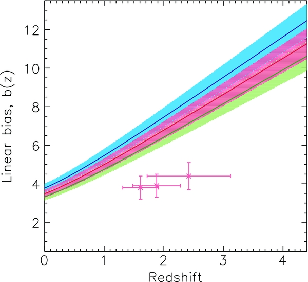
Figure 8. Redshift-dependent best-fit linear bias b(z) for three realizations of the B11 model with 1σ error bounds estimated from our MCMC. Also shown are the best-fit single-value linear biases found in V09 for the BLAST 250, 350, and 500 μm auto-spectra, plotted at median redshifts z = 1.61, 1.88, and 2.42, respectively.
Download figure:
Standard image High-resolution imageOur choice of source model and bias parameterization is likely affecting b(z). The B11 model contains two distinct classes of IR sources, "normal" and "starburst," with substantially different luminosities, which is not accounted for in our b(z) parameterization. Also, the B11 model does not match observational constraints equally well across the whole wavelength range probed by ACT and BLAST; for instance, it underpredicts Poisson power and number counts compared to BLAST and South Pole Telescope (SPT) measurements at 500 and 1360 μm (see Section 5.6 of Béthermin et al. 2011, as well as Figure 9 of this paper). An underprediction of dI/dz would result in a higher bias to compensate.
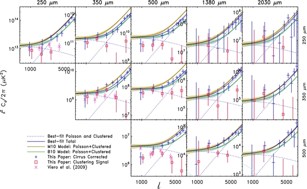
Figure 9. BLAST × BLAST (250–500 μm) and ACT × BLAST (1380–2030 μm) power spectra in ℓ2Cℓ/2π. Data, which have had Galactic cirrus power removed, are shown as blue crosses. Red squares are the same data after removal of the Poisson term, and after logarithmic binning, with log(Δℓ) = 0.2, and represent the contribution to the total power spectrum from clustering. Pink exes are the clustered term data from V09. The blue dotted lines rising to larger ℓ are the best-fit Poisson terms, and the approximately horizontal blue dotted lines are the best-fit clustering terms, which are determined by the z-dependent bias, as described in Section 6. Also plotted are the phenomenological models of B11 and M11, in green and brown (with shaded error regions), respectively. Poisson levels are calculated after truncating the counts at 300, 250, 170, 20, and 20 mJy at 250, 350, 500, 1380, and 2030 μm, respectively. Error regions are calculated with Monte Carlos. Both the models agree at some effective wavelengths, but disagree at others, so that neither describes the data fully. The M11 model also somewhat overpredicts the CIB at BLAST wavelengths, which is consistent with the behavior of the model Poisson term here. Note that the vertical scale is different for each panel. The cirrus-corrected data here are given in Table 2.
Download figure:
Standard image High-resolution image7. DISCUSSION
We compare the models of B11 and M11 (described in Section 2.3) to our results. Poisson levels are calculated from the number counts using Equation (4), where the values of Scut are chosen to mimic those used in the analysis, i.e., Scut = 500, 250, and 170 mJy at 250, 350, and 500 μm, respectively.
Model predictions of B11 and M11 are shown in Figure 9 as green and brown lines with shaded error regions, respectively. Both models agree at some effective wavelengths, but disagree at others, so that neither appears to fully describe the data. The M11 model also somewhat overpredicts the CIB at BLAST wavelengths, which is consistent with the behavior we see for the model Poisson term. On the other hand, as already mentioned, the B11 model underpredicts Poisson power and number counts compared to BLAST and SPT measurements at 500 and 1360 μm, which again is consistent with the behavior of the Poisson term of the model in Figure 9.
The Poisson and clustered power amplitudes are plotted as a function of effective wavelength, defined as  , in Figure 10. Also included are measurements made by the following experiments: AKARI at 90 μm (Matsuura et al. 2011); Spitzer at 160 μm (Lagache et al. 2007); BLAST at 250, 350, and 500 μm (Viero et al. 2009); ACT at 1380, 1673, and 2030 μm (Dunkley et al. 2011); SPT at 1363, 1629, and 1947 μm (Hall et al. 2010); and the FIRAS modified blackbody (T = 18.5, β = 0.64), which is shown as a dotted line.
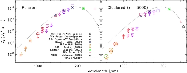
Figure 10. Cℓ vs. wavelength for observations and models. From left to right, the actual or effective wavelengths,  , (in μm) are 2030, 1673, 1380, 1007, 843, 831, 712, 695, 587, 500, 418, 354, 350, 296, 250, 160, 100, and 90. Best-fit Poisson (left panel) and clustered (at ℓ = 3000, right panel) Cℓ from measurements are shown as squares (auto-spectra) and diamonds (cross-spectra), respectively, and our measurement of IRIS galaxies is shown as red crosses. Open circles represent the prediction for the clustered power at the ACT wavelengths from the best-fit, redshift-dependent bias model. Uncertainties are omitted for visual clarity, but are generally smaller than the size of the symbols due to the large dynamic range in Cℓ. The geometric mean of the cross-band spectra, defined as
  , are shown as downward-pointing arrows. Measurements from other experiments are ACT (Dunkley et al. 2011, yellow asterisks); BLAST (Viero et al. 2009, black exes); Spitzer (Lagache et al. 2007, green asterisk); SPT (Hall et al. 2010, yellow triangles); and AKARI (Matsuura et al. 2011, black triangle). The FIRAS modified blackbody (T = 18.5, β = 0.64) is plotted as a dotted line. As was seen in Hall et al. (2010; Figure 5), FIRAS describes the data short of 500 μm, but overpredicts the measurements at millimeter wavelengths. The ratio of the measurement (diamonds) to the geometric mean (downward-pointing arrows) represents the level of cross-correlation between bands.
Download figure:
Standard image High-resolution imageThe degree of correlation between widely spaced wavelengths is of interest both in determining the redshift distribution of sources, and for modeling the IR source power as a CMB contaminant. To assess the correlation, the geometric means at each effective cross-band wavelength, defined as  , are shown as a downward-pointing arrow. Since we do not measure Cλℓ at λ = 1380 and 2030 μm, we rely on measurements by Dunkley et al. (2011) for those bands when calculating the geometric means. The ratios of the measurements to the geometric means,
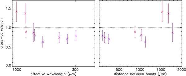
  , then represent the levels of cross-correlation between bands. These are shown in Figure 11 for the Poisson power as a function both of effective wavelength and of distance between bands. Correlation is seen between all the frequencies and does not fall significantly as a function of increased band separation, suggesting a tight redshift distribution for the overlapping population. This behavior is consistent with Hall et al. (2010) and Dunkley et al. (2011), who found that the 1000–2000 μm bands are correlated at close to the 100% level.
Figure 11. Left panel: cross-frequency correlation vs. effective wavelength for Poisson. Cross-frequency correlation is defined as Cλλ'ℓ/(Cℓλ Cλ'ℓ)1/2, i.e., the ratio of the measurement (diamonds in Figure 10) to the geometric mean (downward-pointing arrows in Figure 10). Note that, as in Figure 10, the ACT × BLAST Poisson level geometric means are calculated from auto-frequency correlation levels derived with the ACT × BLAST mask. From left to right, the actual or effective wavelengths,  , (in μm) are 2030, 1673, 1380, 1007, 843, 831, 712, 695, 587, 418, 354, and 296. The horizontal line at unity represents 100% cross-correlation. Right panel: cross-frequency correlation vs. distance between bands. Correlation is seen between all the ACT and BLAST frequencies.
Download figure:
Standard image High-resolution image
8. CONCLUSION
We present measurements of the auto- and cross-frequency correlations of BLAST (250, 350, and 500 μm) and ACT (1380 and 2030 μm) maps. We find significant levels of correlation between the two sets of maps, indicating that the same DSFGs that make up the unresolved fluctuations in BLAST maps are also present in ACT maps. Furthermore, we confirm previous BLAST analyses (Viero et al. 2009) for a different field and with an independent pipeline, and extend the analysis by including BLAST × BLAST cross-frequency correlations.
We fit Poisson and clustered terms at each effective wavelength simultaneously, which we achieve by adopting a model for the sources (Béthermin et al. 2011), assuming a parameterized form for the z-dependent bias and using an MCMC to minimize the χ2. Using this model we detect a clustered signal at 4σ, in addition to a Poisson component. The best-fit bias is one that increases sharply with redshift and is consistent with what was found by Viero et al. (2009).
We compare phenomenological models by Béthermin et al. (2011) and Marsden et al. (2011) to the data and find rough agreement at numerous effective wavelengths. But we also find that neither model quite reproduces the data faithfully. Thus, we expect this measurement and others like it will ultimately provide powerful constraints for the redshift distribution and SEDs of future versions of the models.
Though we find convincing evidence for correlated Poisson and clustered power from DSFGs, the levels of precision needed to robustly remove these signals from CMB power spectra demand better measurements still. This is particularly true of the clustering term, whose contribution to the power spectrum in ℓ2Cℓ peaks at ℓ ∼ 800–1000, which is also the region in ℓ-space typically targeted in searches for the SZ power spectrum. Since the clustered term should scale independently of the Poisson term, the measurement becomes increasingly important to determine precisely. Future studies combining Herschel/SPIRE with ACT, SPT, and Planck will go a long way toward solidifying this much needed measurement.
BLAST was made possible through the support of NASA through grant Nos. NAG5-12785, NAG5-13301, and NNGO-6GI11G, the NSF Office of Polar Programs, the Canadian Space Agency, the Natural Sciences and Engineering Research Council (NSERC) of Canada, and the UK Science and Technology Facilities Council (STFC). C.B.N. acknowledges support from the Canadian Institute for Advanced Research.
ACT was supported by the U.S. National Science Foundation through awards AST- 0408698 for the ACT project, and PHY-0355328, AST- 0707731, and PIRE-0507768. Funding was also provided by Princeton University and the University of Pennsylvania. Computations were performed on the GPC supercomputer at the SciNet HPC Consortium. SciNet is funded by the Canada Foundation for Innovation under the auspices of Compute Canada; the Government of Ontario; Ontario Research Fund–Research Excellence; and the University of Toronto. J.D. acknowledges support from an RCUK Fellowship. S.D., A.H., and T.M. were supported through NASA grant NNX08AH30G. A.K. was partially supported through NSF AST-0546035 and AST-0606975 for work on ACT. E.S. acknowledges support by NSF Physics Frontier Center grant PHY-0114422 to the Kavli Institute of Cosmological Physics. S.D. acknowledges support from the Berkeley Center for Cosmological Physics. We thank CONICYT for overseeing the Chajnantor Science Preserve, enabling instruments like ACT to operate in Chile; and we thank AstroNorte for operating our scientific base station. Some of the results in this paper have been derived using the HEALPix (Górski et al. 2005) package.
The authors thank Matthieu Béthermin and Guilaine Lagache for their help.
APPENDIX A: UNIT CONVERSION
The flux density unit of convention for infrared, (sub)millimeter, and radio astronomers is the Jansky, defined as

and is obtained by integrating over the solid angle of the source. For extended sources, the surface brightness is described in Jy per unit solid angle, for example, Jy sr−1, (as adopted by BLAST), or Jy beam−1 (e.g., SPIRE). Additionally, the power spectrum unit in this convention is given in Jy2 sr−1.
CMB unit convention is to report a signal as δTCMB; the deviation from the primordial 2.73 K blackbody. To convert from Jy sr−1 to δTCMB in μK, as a function of frequency:
(Fixsen 2009). Because the BLAST bandpasses have widths of ∼30% (Pascale et al. 2008), and because the CMB blackbody at these wavelengths is particularly steep (falling exponentially on the Wien side of the 2.73 K blackbody), the integral of δBν/δT over the bands is weighted toward lower frequencies; an effect that becomes dramatically more pronounced at shorter wavelengths. Thus, the effective BLAST band centers in δT are ∼264, 369, and 510 μm, leading to factors of conversion from nominal of ∼2.46, 1.75, and 1.13, respectively.
Lastly, the CMB power spectrum is conventionally reported versus multipole ℓ, while in the (sub)millimeter the convention is to report it versus angular wavenumber, kθ = 1/θ, which is also known as σ in the literature, and is typically expressed in arcmin−1. In the small-angle approximation the two are related by ℓ = 2πkθ.
APPENDIX B: POWER SPECTRUM UNCERTAINTIES
The contents of each map used for cross-frequency correlations can be considered as a sum of two parts: one with a finite cross-correlation and the other with vanishing cross-power spectrum. The former contributes to the signal in the cross-power spectrum, while the latter contributes to the uncertainties. Therefore three terms contribute to the power spectrum uncertainties: sample variance in the signal due to limited sky coverage, the noise, and a non-Gaussian term due to the Poisson-distributed compact sources and galaxy clusters. The diagonal component of the ACT × BLAST cross-spectrum variance can be written as the sum of these terms, in order
where  , estimates the average power spectrum of the noise; the superscripts (1) and (2) label the maps (1 for ACT, 2 for BLAST); nb counts the number of Fourier modes measured in bin b (that is, the number of pixels falling in the appropriate annulus of Fourier space); fsky is the patch area divided by the full-sky solid angle, 4π sr; and
  is the mean cross-spectrum. The last term, σ2P, arises from the Poisson-distributed components in the maps (i.e., unresolved compact sources and clusters of galaxies) and is given by the non-Gaussian part of the four-point function as described in Fowler et al. (2010) and Hajian et al. (2010). For purposes of the covariance calculation, we assume that the spatial distribution of these objects is uncorrelated. This term is constant with ℓ.
The noise terms in the ACT and BLAST maps are given by
where CRGb is the power spectrum of the radio galaxies in the ACT maps and NAb and NBb are the noise spectra in ACT and BLAST, respectively. The noise terms, Nb, are dominated by the atmospheric noise on large angular scales and by detector noise on the smallest scales (Das et al. 2011). The CMB is a major source of noise for this study out to ℓ ∼ 2500, especially for the 148 GHz data. Radio galaxies only contribute to the uncertainties through the fourth moment of the field. They do not bias the signal. The effect of the radio galaxies is stronger at 148 GHz and is negligible at 218 GHz. Therefore, we mask the brightest radio galaxies in the 148 GHz map to reduce the uncertainty on the cross-power spectra.
The uncertainties on BLAST × BLAST power spectra are computed using a similar analytic estimate, given in Equation (9) of Fowler et al. (2010) with nw = 6 cross-spectra per map.
As a sanity check, we compare our analytic estimate of the error bars with the standard deviation of the power spectra computed from patches of the sky. We divide the data into four patches of equal area and with them compute four independent cross-power spectra. We use the variance of the measurements at each ℓ bin as a measure of the error on the power spectrum. This method agrees well with the analytic estimate of the errors; however, due to the small area of the sky used in this analysis, both analytic and patch-variance estimates of the error bars have uncertainties which are limited by fsky. Thus, we conservatively use the greater of the analytic and patch variances as an estimate of the uncertainty of the power spectrum. We test the effect that this choice of error bars has on our results in Section 6.1.
When fitting parameters, we take the joint likelihood function to be diagonal as the off-diagonal elements are small (Das et al. 2011).
Footnotes
- 26
ACT Collaboration papers are archived at http://www.physics.princeton.edu/act/ .
- 27
BLAST results and publications can be found at http://blastexperiment.info/ .
- 28
- 29
HCON refers to each individual observation at three different epochs. For more information, and publicly available maps, see http://www.cita.utoronto.ca/mamd/IRIS/.
- 30