

Abstract
This work aims to make three-dimensional (3D) tomographic techniques more flexible and accessible to in-situ measurements in practical apparatus by allowing arbitrary camera placements that benefit applications with more restrictive optical access. A highly customizable, in-house developed tomographic method is presented, applying smoothness priors through Laplacian matrices and hull constraints based on 3D space carving. The goal of this paper is to showcase a reconstruction method with full user control that can be adopted to various 3D field reconstructions. Simulations and experimental measurements of unsteady premixed CH4/air and ethanol (C2H5OH) diffusion pool flames were evaluated, comparing arbitrarily placed cameras around the probed domain to the more commonly used in-plane-half-circle camera arrangement. Reconstructions reproduced expected topological field features for both flame types. Results showed slight decrease in reconstruction quality for arbitrarily placed cameras compared to in-plane-half-circle arrangement. However, at lower numbers of camera views (Nq ⩽ 6) arbitrary placement showed better results. The introduced methodology will be useful for optically limited setups in terms of handling a priori information, camera placement and 3D field evaluation.
Export citation and abstract BibTeX RIS

Original content from this work may be used under the terms of the Creative Commons Attribution 4.0 license. Any further distribution of this work must maintain attribution to the author(s) and the title of the work, journal citation and DOI.
1. Introduction
Advancement in areas of science and technology look for constant improvement and development of measurement techniques to cover both specific problems and to increase flexibility and applicability. Research in combustion related areas such as modeling, device performance or pollutant reduction require detailed experimental flame studies. Improvements can lead to better efficiency in many energy conversion processes and allow for new alternative fuels to be utilized. Studies of flame position and topology, that is crucial for determining heat transfer and flame quenching, is important together with other processes such as ignition or stabilization, especially for less studied alternative fuels. Similarly, reduction of harmful pollutants including soot and NOx emission is not only important to combat global warming but also to reduce risks to human health [1].
However, the inherent three-dimensional (3D) nature of flames calls for accurate and versatile measurement techniques. Enhanced 3D flame information can, for example, help to further improve existing burner devices and their designs. Multiple well-established techniques exist for acquiring 3D flame information but many of these techniques produce time averaged or spatially interpolated information from multiple planar measurements such as two-dimensional (2D) laser-induced fluorescence imaging [2, 3]. Solutions for time and spatially resolved measurements utilizing scannable lasers and high-speed cameras exist, but such equipment is expensive and its application in turbulent flame conditions can be a challenge. Therefore, alternative non-intrusive diagnostic techniques, that have the potential to allow for both spatially and temporally resolved 3D flame information is of high interest.
A 3D tomographic reconstruction is one such measurement technique that has been applied in multiple fields such as medicine, chemistry, biology, and fluid dynamics. Typically, this approach is employed to 3D geometries, movements, flow fields and species distributions. Although the presented approach with arbitrary camera positions can be universally applied, 3D flame visualization is here being used for proof-of-concept. Volumetric flame field measurements utilizing tomographic methods have seen an increase of use within the field of combustion diagnostics due to its non-intrusive nature and ability to estimate 3D flame information [4]. Further, combination with other measurement techniques such as laser absorption spectroscopy [5, 6], particle image velocimetry [7] schlieren techniques [8, 9] or volumetric laser-induced fluorescence [10â12] has proven fruitful. The technique allows improvements on 3D measurements focusing on flame features such as flame position, topology, species location, acoustic oscillations, soot formation, and soot volume fraction for not only laminar, but also unsteady and turbulent flames.
Spatially reconstructing 3D flame chemiluminescence (CTC) fields emitted from different excited species during combustion, such as CO*, C2*, CH*, and OH*, can greatly help investigate flame properties like flame propagation, geometry, wrinkling, curvature, surface density and identification of recirculation or precession zones. Especially the study of CH* and OH* is important, as they are known markers for reaction and post flame zone respectively. Floyed et al initially introduced computed tomography of CTC by reconstructing a premixed CH4/air flame in three dimensions using multiple camera views and also extended it to reconstruction of CH* field in a CH4 and O2 matrix burner flame [13, 14]. Combined with high-speed imaging, the technique has been used to acquire temporally resolved OH fluorescence fields [10] and measurements of combustion intermediates such as polycyclic aromatic hydrocarbons and CH2O [15]. A 3D temperature measurements have likewise been performed combining the technique with two-line OH excitation [11]. Measurements of 3D soot volume fraction in turbulent jet diffusion flames were studied by Meyer et al [16] showing the versatility of the technique.
At the heart of the tomographic technique lies an inverse problem and one of the most used solvers, in the field of combustion diagnostics, is the algebraic reconstruction technique (ART), known for allowing easy implementation of a priori information in between iterations [13, 17]. Other algorithms have similarly been utilized due to individual strengths, a few examples include simultaneous ART with increased parallelizability [18], multiplicative ART or its simultaneous counterpart that due to their multiplicative nature always keeps zero intensity values as zero, beneficial in some flame field topologies [10, 16, 19]. Moreover, stochastic methods have sometimes been used for solving the 3D tomographic problem [20].
The general robustness of tomographic methods, when applied in combustion diagnostics, has been investigated through comparisons of flame topology measurements made by 2D planar laser-induced fluorescence and 3D CTC tomography [12, 21]. Moreover, in-depth studies on tomographic reconstructions of a turbulent swirl burner and the effect of projection view number, voxel resolution and in plane camera placement was performed by Mohri et al [4]. These studies showcase good reliability and future promise for technique application in studies of 3D flame properties. However, each application is unique and may present different challenges and trade-offs, thus warranting fully customizable tomographic methods to maintain control.
However, most 3D tomographic flame field studies have been performed in well controlled laboratory environments without much restriction in terms of optical access. Similar to other optical techniques that have been applied in practical environments [22â24], the act of transferring the measurement setup from a laboratory environment to practical devices and performing in-situ diagnostics, can be challenging. One example of such a practical application where in-situ 3D tomographic flame field studies could be performed, requiring flexible camera placements, is the marine engine cylinder head with 24 optical access ports shown in figure 1.
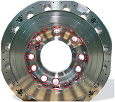
Figure 1. Image of cylinder head for large bore marine engines with 24 optical access ports (marked by red circles). Reproduced with permission from John Hult, MAN Energy Solutions.
Download figure:
Standard image High-resolution imageFactors such as restricted optical access, hindering the placements of cameras at certain positions, reduction in field of view of individual cameras, diminishing sensitivity due to window fouling or image overexposure due to insufficient dynamic range of sensors all contribute to the difficulty.
Work has previously been done looking into tomographic reconstructions with a restricted field of view [25] and over-exposure compensation [26]. In cases where optical access has to be achieved in practical apparatus, the geometry would rarely allow for the in-plane-half-circle camera arrangements that has been used in most previous experimental measurements or mirror arrangements using dual or quad scopes [10, 27]. Instead, arbitrarily placed cameras would most likely be required to accommodate any available optical access. But position of acquired projections will affect the measurement quality as highlighted by Grauer et al [28] when investigating optimal optical path arrangement in absorption tomography. This poses a challenge on equipment size, calibration procedures and reconstruction methods. Studies using endoscopic arrangement, applying fiber bundles, have previously been performed [29, 30]. Such setups could perhaps, with modifications, be suited for arbitrary placement. The effect of variable camera placements on 3D tomographic reconstructions have previously been explored by Cai et al [31] using a single movable camera. Further, Wang et al [32] performed numerical investigations looking at optimizing camera placement in case of constrained optical access. However, the effect on tomographic flame field reconstruction with multiple arbitrarily placed cameras combining simulative and experimental measurements have, to the best of the authors knowledge, not been investigated.
This work aims to enhance applicability of the tomographic technique for in-situ, non-intrusive, volumetric flame measurement based on CTC by facilitating and evaluating the effects of arbitrarily placed cameras. The work also presents options for enhancing reconstruction quality and allow scenario specific customization to the overall tomographic procedure with regard to incorporating prior knowledge, something not always feasible when employing commercial solutions. This comes in terms of hull constraints, based on space carving, and smoothness priors through Laplacian matrices in the reconstruction process. Experimental reconstructions made using small commercially available complementary metal-oxide-semiconductor (CMOS) cameras as well as simulative comparisons between different camera arrangements were conducted. The experimental measurements show premixed CH4/air Bunsen burner flames as well as small ethanol (C2H5OH) pool flames, allowing for both well defined, steady, and unsteady flames to be studied yielding a broader result spectrum, when investigating the effect of arbitrarily placed cameras. This work applies a highly customizable, in-house developed tomographic method, using a preconditioned conjugate gradient (PCG) solver. The goal is to present a reconstruction process that can be fully or partially adopted to various flame field reconstructions and to discuss important aspects regarding reconstructions such as benefits and trade-offs in terms of prior knowledge and camera placements.
2. Method
The general method behind 3D tomographic reconstructions of CTC revolves around the simultaneous acquisition of multiple 2D projection measurements of the probed domain  . Each individual view projection
  is acquired at a different viewing angle and position surrounding the investigated domain and is made up of multiple
  pixel projections
  , illustrated in figure 2. In this work the continuous domain
  is spatially discretized into
  voxels for computational purposes.
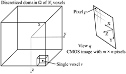
Figure 2. Illustration of 2D view projection and probed domain  , discretized into
  voxels.
Download figure:
Standard image High-resolution image2.1. Principle of reconstruction model
The studied intensity within the domain  at locations
  can be described as a continuous field
  . Flame intensity distribution can be mapped to the projection measurements
  , acquired by the optical setup, through a Fredholm integral equation of the first kind given by the radiative transfer equation (RTE) [33],
where  is the continuous flame field and
  is a projection measurement from view
  and pixel
  . Furthermore, a smoothness requirement, corresponding to a smoothing spline [34, 35], was applied in this work to the flame field by introducing a penalty term as
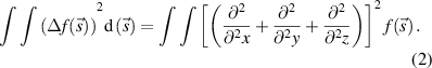
Minimizing the second derivative throughout the flame field, resulting in more continuous solutions, which is physically expected in the studied flames while also alleviating any negative effects due to an ill-posed problem. This allows the final reconstruction problem to be stated as
where,  is the weight of the penalty term and the minimization finds the reconstruction that best balances observational measurements against the applied smoothness requirement. The parameter
  can either be found empirically by trial and error or estimated [36].
Discretization of the studied flame field into a voxel scalar field allows the RTE integral, seen in equation (1), to be approximated as a finite sum over the flame field, yielding a projection approximation of each intensity measurement  as
as
where  is a voxel,
  that voxel's contribution to the projection
  and
and  defining a line-of-sight projection of said voxel
  . Equally, the smoothness prior in equation (2) can be represented by a sparse discrete Laplacian matrix:
where  ,
,  and
and  are one-dimensional (1D) discrete Laplacian.
  ,
,  and
and  are identity matrices of applicable size. Here each 1D discrete Laplacian applies a homogenous Dirichlet boundary condition which results in a final 3D discrete Laplacian with homogenous Dirichlet boundary condition for all boundaries specified by

with  being the boundary of the domain. The continuous problem can then be reformulated in a discretized form [37] as follows

Here  is a projection matrix containing all linear voxel projections and
  is the unknown field vector i.e. the discretization of
  . The discretized reconstruction of the probed domain
  is given by the solution to the minimization problem in equation (7), this is a quadratic problem with known closed form solution [35]:

which is best solved using iterative methods [38] to avoid costly matrix operations.
An alternative interpretation of the latter part of the discretized system in equation (7) is as a prior latent Gaussian field [39] with precision matrix given by  for the domain
  and observations given by the discretized integral in equation (4). The resulting model is

where  are independent observational and discretization errors with variance
  for each pixel and
  is a smoothness weight. The posterior for the discretized domain
  , conditional on observations and parameters is then given by
with the conditional expectation being

Taking  this becomes identical to the optimal reconstruction in equation (8). Note that individual values of
  and
and  are not needed for the reconstruction. An advantage of formulating the model in a statistical framework is the ability to quantify the uncertainty in the reconstruction as

This variance requires individual values for  and
and  and computation of the matrix inverse is likely to require iterative and/or approximate methods [40]. Investigation of the uncertainties is outside the scope of this paper, but the theoretical results and possible numerical methods are provided here for completeness.
2.2. Principle of imaging model
The mapping of 2D camera projection measurements to each respective voxel was built around the pinhole camera model introduced by Tsai [41], that is a highly used model in the field of computer vision. This produced a versatile way of tracing camera rays as well as reducing barrel or pincushion distortions on the camera images [42, 43]. This model computes two matrices, seen in equation (13), based on calibration measurements. One intrinsic matrix  with information regarding principal point
  , camera focal length
  , and camera axis skew
  . The second is the extrinsic matrix
  , a rigid transformation matrix with the camera rotation
  and translation vector
  :
:
These two matrices facilitate the relationship between a point  in 3D space expressed in homogeneous coordinates located in the probed domain
  and a projection point
  in the detection cameras pixel domain:

where  is a scaling factor. This method allows for high flexibility when it comes to camera placements which is beneficial for arbitrary placed cameras to accommodate limited optical access. Each individual voxel
  in the discretized domain is sampled multiple times by projection of randomly placed points from within the voxel onto the camera sensors, similar to methods used by Liu et al [25] and Yu et al [25, 44]. This yields intensity contribution weights
  from each voxel
  to each sensor measurement
  . Voxels tend to be larger than camera pixels, although this depends on voxel size, camera distance and resolution of the cameras used; as a result, each voxel can project to more than one pixel. Intensity contribution weights
  are given by the number of sample points projected onto a specified pixel in relation to the total number of sample points used. These contributions can then be reshaped into a sparse projection matrix
  .
.
This work took advantage of paraxial approximation previously used in [4, 45], namely assuming that the angle between the optical axis of each projection ray is small, granting close to orthographic projections of each voxel due to parallel rays. This approximation greatly speeds up computation time and is deemed valid if the distance between the lens and the probed domain is not too small. Aliasing effects due to domain discretization can be a problem, resulting in unwanted frequency patterns in the projection mapping. In this work aliasing and the resulting reconstruction artifacts were reduced by randomly moving each voxels sampling coordinates slightly before projection, thus reducing effects caused by the discretization structure.
The projection model described in equation (1) is a simplification of the RTE in terms of scattering, self-absorption, and background intensity. The experimentally studied flames were first premixed CH4/air flames, such flames can be considered optically thin, since they have very low soot production. Small ethanol pool flames were later studied and similarly showed a low soot production albeit more than the premixed ones. Having a small flame size in all cases and the cameras placed not far from the flame yields low scattering conditions that have negligible effects allowing scattering to be excluded from the model. Self-absorption was neglected due to the main source of emission being visible CTC from CH*, mainly from the transition  and this particular transition is judged to suffer negligible self-absorption effects [46, 47]. This same assumption is reasonable for other flame CTC sources in the visible region, in comparison to OH which is known to have large self-absorption [14, 46]. However, it is important to evaluate every experimental situation individually.
Many inverse problems, such as tomographic flame field reconstruction, are notorious for being ill-posed. Depending on the ratio between the number of optical projection measurements and domain voxels the resulting linear system can be either underdetermined or overdetermined. Flame tomography problems also tend to be ill-conditioned due to domain discretization and effects from such errors will be amplified in the measurements  [8, 33]. Therefore, adding a priori information and boundary conditions to the reconstruction process limits the possible solutions to those that produce more correct estimates of the flame field. The application of smoothing in flame reconstructions, based on the assumption of a continuous field, helps in this regard. For more complex fields such as turbulent flames that require very high temporal and spatial resolution the same would be true however reconstructions could perhaps suffer a trade of between resolving finer spatial features or having a more overall correct flame field estimate. Solutions to this could involve adding more projections or applying more flexible smoothing models that allow for varying dependence strength between voxels [48], but this might add complexity to the reconstruction due to the need for additional parameter estimation that control the non-stationary smoothing. In this work, to further enhance quality and computational speed, a hull-constraint, based on space-carving, was applied to the probed domain prior to reconstruction [49â51]. The space-carving worked by projecting each voxel onto all cameras and if any voxel projects to a total pixel area with zero intensity in any individual camera that voxel is removed from the domain. This removes voxels that are known to have zero intensity prior to the reconstruction which reduces the system size while retaining the overall flame shape. Zero intensity voxels close to the flame are kept, giving flexibility in the systems solution process. In terms of memory requirements, the sparse smoothing matrix
  is a large
  -by-
-by- matrix but the number of non-zero elements is small. With the smoothing operator only including the six direct voxel-neighbors every row of the
  matrix will only contain seven non-zero elements (the voxel itself and the six neighbors). Storing such a sparse matrix requires around 250 Mb of memory, depending on
  . The final sparse projection matrix
  will be
  -by-
-by- mapping the
  voxels to the pixels in all image planes. Since each measurement represents a camera ray going through the domain volume each row of
  has roughly
 ![$\sqrt[3]{{{N_v}}}$](https://content.cld.iop.org/journals/0957-0233/33/12/125206/revision2/mstac92a1ieqn76.gif) non-zero elements. In practice, for a case with ten cameras,
non-zero elements. In practice, for a case with ten cameras,  has initially about
  non-zero elements and requires around 1 Gb of storage which then is reduced by space carving. The reduction depends on flame size, but for cases studied here 10%â25% is commonly achievable.
This work applied the preconditioned conjugate gradient (PCG) method to solve the resulting inverse problem mainly due to high computational performance and implementation ease. Non-negativity restriction was achieved by iteration of the PCG algorithm with voxels containing negative intensity in previous results being iteratively removed, although convergence is not guaranteed using this method, simulations and visual inspection of experimental reconstructions showed good results and consistency. The stopping criteria for determining convergence was a tolerance on the relative residuals  . Here the relative tolerance was set to
  and a maximum number of allowed iterations to
  . For all cases, the algorithm terminated based on tolerance after around 55â120 iterations, for larger systems additional iterations may be needed. The method was implemented using MATLAB version 2020b and the computational cost for field reconstruction using this method is divided between two steps. First, the computation of projection matrix
  which only needs to be performed once for each camera setup. In the case of ten cameras, the computational time was around 10â30 s but may increase as it is dependent on the number of voxels
  and camera measurements
  . Secondly, reconstruction involving solving equation (8) using a PCG solver. Here the key step is the computation of forward matrix vector products of the form
  with
with  being the current best guess solution. Important is to never form the complete matrix, since
  will be almost completely dense. Instead, only the relevant matrix vector products
  are computed, lowering both computational time and memory requirements. The computational time for the PCG was around 20â30 s in this work.
3. Experimental setup
Flame measurements were performed experimentally using ten CMOS cameras mounted on holders attached to freely movable aluminum poles around the flame target. The holders allowed for a  yaw and
  pitch rotation, enabling both in-plane-half-circle setups and arbitrary camera arrangements with various viewing directions. The camera orientations and positions used in the experimental arbitrary setup can be seen in table 1 and an illustration of one example setup can be seen in figure 3.
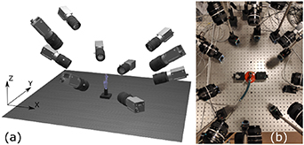
Figure 3. (a) Illustration of an arbitrarily placed camera setup around a burner. (b) Top-down view of experimental setup with similar arbitrary camera placement as illustration.
Download figure:
Standard image High-resolution imageTable 1. List of each cameras yaw rotation, pitch rotation and position used in the arbitrary experimental setup. Acquired by camera calibration.
| Camera # | Yaw (°) | Pitch (°) | Position (X, Y, Z) (mm) | ||
|---|---|---|---|---|---|
| 1 | 91.9 | 68.4 | 23.7, | â257.9, | â99.9 |
| 2 | 150.4 | 45.9 | 217.3, | â101.5, | â227.1 |
| 3 | 115.7 | 47.7 | 113.3, | â196.4, | â211.9 |
| 4 | â159.9 | 51.7 | 215.3, | 87.83, | â159.1 |
| 5 | â123.2 | 46.7 | 144.8, | 204.1, | â222.8 |
| 6 | â85.4 | 64.7 | â3.9, | 263.5, | â114.4 |
| 7 | â65.0 | 49.2 | â83.9, | 231.5, | â219.0 |
| 8 | â37.7 | 55.2 | â153.1, | 144.2, | â154.8 |
| 9 | 49.8 | 48.5 | â129.8, | â162.7, | â200.1 |
| 10 | 13.2 | 47.3 | â194.9, | â34.4, | â203.4 |
The used experimental setup was selected due to being deemed representative of a typical arbitrary setup and also bearing resemblance to the optical access available in the cylinder head for large bore marine engines from MAN Energy Solutions shown in figure 1.
Camera models were Basler acA1920-40gm with monochrome Sony IMX249LLJ-C sensors. Sensor sizes were  by
by  pixels with individual pixel size of
  ×
×  µm. Each camera applied Nikon lenses with a focal length of
  mm using F- to C-mount adapters.
Two flame types were studied, premixed CH4/air Bunsen flames and ethanol as small diffusion pool flames. Example images of each flame at different exposure times are shown in figure 4. The Bunsen burner had an inner diameter of 10 mm. No co-flow or protective shielding was used allowing for somewhat unsteady flames because of ambient motion requiring a shorter exposure to maintain temporal resolution. The ethanol pool flames were burned on 26 mm diameter plates creating wider flames with a little more soot production that were more stable, allowing for longer exposure times.
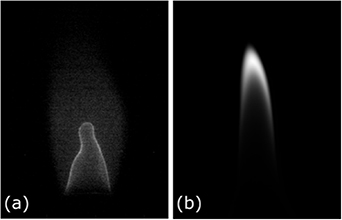
Figure 4. (a) Example image of unsteady premixed CH4/air flame acquired during 200 µs exposure time. (b) Example image of small ethanol diffusion pool flame acquired during 2 ms exposure time.
Download figure:
Standard image High-resolution imageDue to low recorded signal intensity, especially at shorter exposure times in the premixed CH4/air Bunsen flame case, the lenses aperture size was fully opened at a f-number of  to improve the signal-to-noise ratio (SNR) while maintaining sufficient temporal resolution. Varying distance between the flame and cameras due to the arbitrary arrangements made for different depth of fields, however assuming a circle of confusion of 0.03 mm, one of the closer cameras estimates to 22 mm depth of field, enough to cover the volume of interest of both flame cases. Varying camera distances to the probe domain will affect collection efficiency. In this work the effect was judged to be minimal, however in some applications integrating intensity equalization calibration may be needed [10]. Measurements were performed in a dark environment and, where possible, a matt black background was put behind the target flame to enhance image quality while also reducing possible reflections. However, this was not always possible for some camera arrangements. Background images were acquired for each camera with no flame active and subtracted before reconstruction. White field calibration was also performed for each camera.
3.1. Calibration and camera registration
Each camera's orientation and location are required in the imaging model to map voxel projections. This mapping was achieved by computing extrinsic and intrinsic camera matrixes (equation (13)) for each camera through imaging of a calibration target. This work used a checkerboard surface as calibration target, with a square size of 4.05 mm. A minimum of 20 calibration images with unique location and orientation, in relation to each camera, were acquired. The calibration procedure was conducted using the Computer Vision System Toolbox in MATLAB 2020b. During this procedure, image distortions such as barrel and pincushion effects were removed. It should be noted that due to the use of high-quality optics any initial image distortions were observed to be minimal. Finally, multiple images of the calibration target, visible to more than one camera simultaneously, were used to map all cameras to the same coordinate system. Two sets of computed camera locations and orientations acquired from calibration are visualized in figure 5 both for arbitrary camera arrangement (a) and in-plane-half-circle arrangement (b).
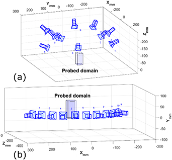
Figure 5. Calibrated camera locations and orientations from experimental arbitrary camera arrangement (a) and in-plane-half-circle arrangement. (b) Probed domain highlighted by the blue box.
Download figure:
Standard image High-resolution imageTo confirm appropriate camera calibration, the reprojection error for each camera was investigated. This is the Euclidian image distance between measured calibration points and the projection of their corresponding estimated points in 3D space from calibration. The mean error was estimated to one pixel for the arbitrary position arrangement in the experimental setup. The effective pixel resolution within the probed domain center was estimated to be  0.01 mm. To increase SNR of the acquired images, image size was reduced by a factor of two resulting in a resolution of
  by
by  pixels and a reduced effective pixel resolution of
  0.02 mm.
4. Simulative study
Simulations were performed to evaluate reconstruction process capabilities with arbitrary camera arrangements as well as the influence of added smoothing prior and hull constraint. The domain of the simulated flame phantom, depicting a hollow Gaussian cone seen in figure 6(a), was discretized into different voxel resolutions with the highest reaching  voxels. The phantom possesses a well-defined structure while still sharing important similarities with an ideal Bunsen flame, such as the hollow interior, allowing straightforward evaluation of reconstruction quality.
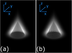
Figure 6. (a) Gaussian cone phantom visualized using final projection method. (b) Gaussian cone phantom visualized using projection method without randomized voxel sampling, aliasing effects are visible.
Download figure:
Standard image High-resolution imageAliasing artifacts due to systematic domain discretization was initially observed in the camera projection model as frequency lines, shown in figure 6(b), resulting in pronounced streak artifacts in the reconstruction domain. Streak artifacts are a common phenomenon in tomography and they were made worse by the aliasing frequency patterns. The implemented routine of randomly moving each voxel's sampling coordinates slightly before projection greatly reduced these aliasing effects as shown in figure 6(a) and in turn streak artifacts in the reconstruction domain diminished.
Slightly shifting voxels in this manner will have minor effects on spatial projection resolution and can be seen as a slight tradeoff between reconstruction resolution and estimation accuracy.
Evaluation for arbitrarily placed cameras was performed by simulating multiple different sets of 20 randomly placed cameras then comparing their individual reconstructions with the original phantom. The allowed camera placements were limited to a half sphere above the flame domain with varying distance to the probed domain center, resulting in similar arrangements as shown in the visualization in figure 3(a) and experimental photo in figure 3(b). Estimation of phantom reconstruction quality was done by looking at two different criteria. The first was root-mean-square-error (RMSE)
where  is the total number of voxels in the reconstruction,
  the simulated phantom and
  the resulting reconstruction. The second was structural similarity index (SSIM), a frequently used index in the field of image analysis that look at dependencies between spatially close voxels [52]
where  is the simulation phantom mean value,
  the reconstruction mean value,
  and
and  the respective variances of simulation phantom and reconstruction,
  the covariance between simulation phantom and reconstruction,
  and
and  are stabilization parameters based on the dynamic range of voxel values.
To investigate the effect of camera view numbers on field reconstruction quality for arbitrary camera arrangements, phantom field reconstructions were made from 50 different camera sets with randomized camera positions. Each camera position in every set where randomized between an azimuth angle of 0°â360° and elevation angle of â45°â45°. Resolution was set to  voxels, similar to resolutions later used in the experimental measurements. Results in terms of RMSE and SSIM are calculated between the full phantom and reconstructed fields are presented in figure 7 with standard deviation based on all 50 different camera sets. In addition, reconstruction results from one in-plane-half-circle arrangement are shown for comparison. Only results produced with between four and 20 cameras are presented as four projections still tend to be able to yield useful field estimates, without too many line artifacts, while a lower number usually results in undesirable quality levels [4].
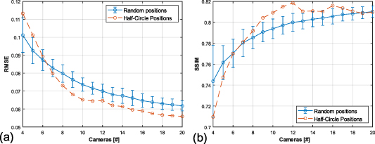
Figure 7. (a) RMSE of phantom reconstructed using simulated randomized camera positions compared to an in-plane-half-circle camera arrangement. (b) SSIM of phantom reconstructed using simulated randomized camera positions compared to an in-plane-half-circle camera arrangement. Error bars represents standard deviation.
Download figure:
Standard image High-resolution imageBetter performance of the in-plane-half-circle arrangement can generally be observed. Most likely due to lower spatial variation between projections, in line with previous studies looking at in-plane camera placement [4]. This confirms that in a well-defined laboratory settings such an arrangement would be preferable. Yet, the difference is not very large, around â¼ , and at lower number of camera views, 4â6, arbitrary positions seem to perform as well or marginally better, up to around â¼
 , where benefits from having input data originating from varied views outweigh the negative effects from increased spatial variation.
Reconstruction results at different voxel resolutions and changing number of camera views from one selected simulated arbitrary camera arrangement are displayed in figure 8. The maximum reconstructed resolution was set to  voxels same as the original phantom resolution. Reconstructed results at lower resolutions were interpolated to match the original phantom resolution to enable comparison. Voxel resolution is shown normalized to the highest resolution and as previously results using between four and 20 cameras are presented.
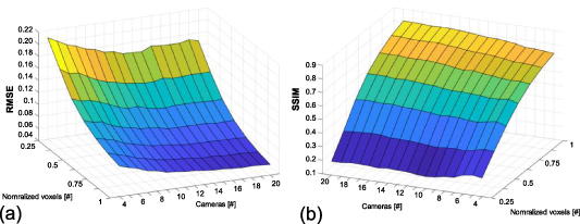
Figure 8. (a) RMSE of simulation phantoms reconstructed with arbitrary camera arrangement. (b) SSIM of simulation phantoms reconstructed with arbitrary camera arrangement.
Download figure:
Standard image High-resolution imageThe expected behavior of better reconstruction estimates with increasing number of camera views at all resolution cases can be observed in figure 8. However, at lower resolution the quality gain from increasing number of camera views is reduced at higher camera numbers, most likely due to the overdetermined problem, with equations heavily outnumbering unknowns and at a point resulting in diminishing quality. Increasing resolution is observed to improve reconstruction quality, due to the higher voxel count, enabling a more accurate field description. However, this improvement will have an upper limit, restricted by the combined information given by the number of projection views, camera resolution, and a priori information.
Figure 9 presents similar reconstruction results of the phantom at a  voxel resolution but now using real experimental camera calibration data from three different arbitrarily as well as in-plane-half-circle arrangements. Figure 9(a) show similar RMSE results as figure 7(a) with the tendency for better reconstructions when applying arbitrary camera arrangements at lower camera numbers. However, this same trend is not seen in the SSIM results in figure 9(b). Further, better estimates yielded with in-plane-half-circle arrangement is supported by the SSIM evaluation but not RMSE evaluation, highlighting the fact that future studies regarding camera mapping and experimental calibration effects would be of interest.
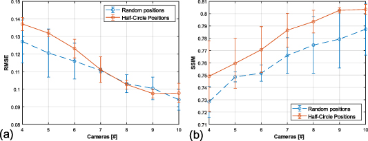
Figure 9. (a) RMSE of phantom reconstruction with different number of cameras for both arbitrary and in-plane-half-circle camera arrangement acquired by real experimental calibration. (b) SSIM of simulation phantom reconstructions with different number of cameras for both arbitrary and in-plane-half-circle camera arrangement acquired by real experimental calibration. Error bars represents standard deviation.
Download figure:
Standard image High-resolution image5. Results and discussion
Laboratory 3D CTC field reconstructions of premixed CH4/air Bunsen burner flames was performed using ten camera views placed at arbitrary positions around the burner, using the geometry shown in figure 5(b). The camera exposure time was set to 200 µs, well below the temporal resolution required to sufficiently freeze the unstable Bunsen flame. Comparisons between original camera images and reconstruction projections at the same view position of a single CH4/air flame measurement are displayed in figure 10. Projection (b) is taken at the same view position as the original camera image (a) that was used in the reconstruction. Similarly, projection (c) corresponds to the original camera image (d), also used in the reconstruction. The hull constraint applied during the reconstruction is visible in projection (b) where intensity originating from above the hull can be observed to accumulate at the top of the reconstructed volume. This is expected and is estimated to have minimal impact to the rest of the reconstruction due to the very low intensities outside the hull. It is well established that projections of a reconstruction acquired at the same view position as a measured camera image used in the reconstruction process will overestimate the quality and resolution of the result. Therefore, this result is intended to showcase the projection method and later results always use projections of reconstructions that do not share a view position with an original camera measurement.
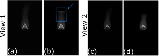
Figure 10. (a) and (c) Original camera measurements of a CH4/air flame used in reconstruction. (b) and (d) Projections of the reconstructed flame made at the same view position as the displayed camera measurements. Effects of applied hull constraint is outlined in (b).
Download figure:
Standard image High-resolution imageThe reconstructed domain was discretized in the x y z dimensions into 100 by 121 by 81 voxels. Flame field reconstructions of the CTC from two different unsteady CH4/air flames are shown in figure 11, depicting each flame's reaction zone at normalized intensity. The part of the flame field facing the reader has been cut away to visualize the ability to capture the expected hollow interior of the Bunsen flames in the reconstructions.
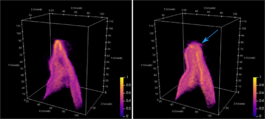
Figure 11. Reconstructed CTC fields depicting the reaction zone of two different experimental premixed CH4/air Bunsen flames. Parts of the field have been removed to show the hollow interior of the Bunsen flames. The luminosity is normalized between 0 and 1.
Download figure:
Standard image High-resolution imageSome minor line artifacts are present in the reconstruction, especially at higher intensity regions such as the top of the flames, highlighted by the arrow, but do not have major impact on the overall flame topology estimation. These results further show that arbitrary camera arrangements, which are more suited for in-situ measurements, can capture individual flame topology of the unsteady Bunsen flame to a satisfactory level in a practical environment.
5.1. Reconstruction convergence
To further test versatility and reconstruction convergence, stable ethanol pool flames were reconstructed using subsets of the ten arbitrarily placed cameras, but with an exposure time of 2 ms increasing the SNR, possible due to the stable nature of the pool flames. Here, a probed domain of 60 by 60 by 200 voxels was applied. Convergence evaluation is important to make sure reconstructions using arbitrary camera arrangements still yield true flame fields estimates. In the following examples, the compared projection viewpoints were not corresponding to any dataset used in the reconstruction process.
Comparison between intensity distributions in two projections made from separate field reconstructions of the same ethanol flame is presented in figure 12. The two field reconstructions are made with different subsets of six cameras each, where two views are shared between the sets. This is akin to the approach used by Meyer et al [16]. The cameras used for reconstruction (1) were 1, 3, 6, 7, 9, 10 and 2, 4, 5, 6, 7, 10 for reconstruction (2). A reference intensity line from field reconstruction using all ten available cameras is shown for comparison.
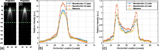
Figure 12. Projections made from two separate field reconstructions (a, 1) and (a, 2) of the same ethanol flame. Intensity is compared between the two projections along one upper and one lower line (light green). (b) Intensity along the upper line for both slices. (c) Intensity along the lower line for both slices. Subsets of six cameras were used, two cameras are shared in-between sets. The projection viewpoint was not part of the reconstruction. The intensity line marked as reference in (b) and (c) corresponds to field reconstruction using all ten available cameras for comparison.
Download figure:
Standard image High-resolution imageThe projections (a, 1) and (a, 2) show similar flame intensity structure and feature size across both lines. However, while the relative intensity is comparable for both projections, the overall absolute intensity can be observed to be consistently lower in reconstruction (1), seen in both (b) and (c). The same intensity difference is observed in comparison between vertical center slices of the same two reconstructions, displayed in figures 13(a, 1) and (a, 2), acquired from the same viewpoint at previous projections in figure 12. Here one can further spot small structural differences such as the minor intensity spike at â¼ voxels in figure 13(c) visible in reconstruction (1) but not visible in (2). The flame intensity structure follows the reference reconstruction for both (1) and (2) but differences in intensity exist for both.
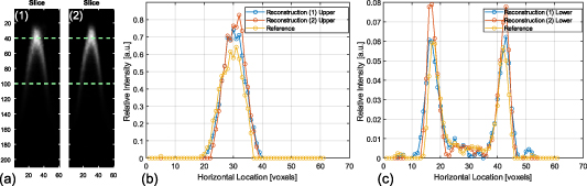
Figure 13. Vertical center cross section slices from two separate field reconstructions (a, 1) and (a, 2) of the same ethanol flame. Intensity is compared between the two slices along one upper and one lower line (light green). (b) Intensity along the upper line for both slices. (c) Intensity along the lower line for both slices. Six cameras were used, two cameras are shared in-between sets. The slice viewpoint was not part of the reconstruction. The intensity line marked as reference in (b) and (c) corresponds to field reconstruction using all ten available cameras for comparison.
Download figure:
Standard image High-resolution imageIt is important to understand the limitations coming with arbitrary camera positions, therefore the same flame field as in figure 12 was again reconstructed, but now using subsets of four cameras each where no camera was shared between the sets. Here cameras 1, 2, 3, 4 was used for reconstruction (1) and 7, 8, 9, 10 for reconstruction (2). This is a low number of projection views and noticeable effects on results are expected. Results show that major structures remain comparable between the reconstructions, but differences are more common and pronounced. Such a difference is notably seen in the lower dashed lines presented in figure 14(c). Here the central intensity decrease, at around â¼ voxels, behaves differently between the two reconstructions. Furthermore, the first reconstruction (1) no longer has consistently higher intensity than the second reconstruction (2), observed in both in figures 12(b) and (c), indicating error in the relative intensity. Also, the intensity differences between the reference reconstruction and both reconstructions (1) and (2) are now larger further suggesting higher error as expected.
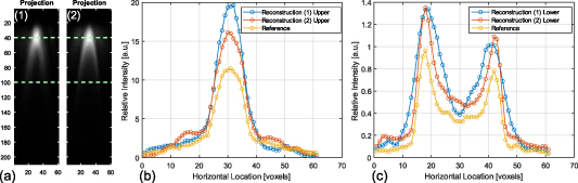
Figure 14. Projections made from two separate field reconstructions (a, 1) and (a, 2) of the same ethanol flame. Intensity is compared between the two projections along one upper and one lower line (light green). (b) Intensity along the upper line for both slices. (c) Intensity along the lower line for both slices. Four cameras were used, no cameras are shared in-between sets. The projection viewpoint was not part of the reconstruction. The intensity line marked as reference in (b) and (c) corresponds to field reconstruction using all ten available cameras for comparison.
Download figure:
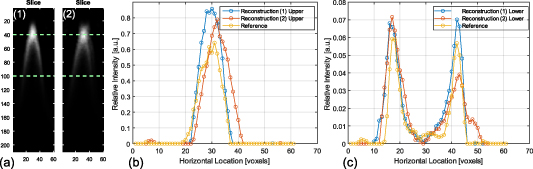
Standard image High-resolution imageFurther reconstruction disparity is more apparent between the vertical slices presented in figure 15. Here even larger flame structures are shown to be affected, seen both in the varying flame position between the slices (a) and in the intensity distributions of the upper dashed lines (b). Similar flame structure still remains between the lower dashed lines (c), but intensity variations can still be observed in the right peak together with artificial broadening.
Figure 15. Vertical center cross section from two separate field reconstructions (a, 1) and (a, 2) of the same ethanol flame. Intensity is compared between the two slices along one upper and one lower line (light green). (b) Intensity along the upper line for both slices. (c) Intensity along the lower line for both slices. Four cameras were used, no cameras are shared in-between sets. The slice viewpoint was not part of the reconstruction. The intensity line marked as reference in (b) and (c) corresponds to field reconstruction using all ten available cameras for comparison.
Download figure:
Standard image High-resolution image
The observed relative intensity difference visible in figure 12 is believed to be the result of using only six cameras, still relatively few camera views and the difference is expected to disappear with increased number of cameras. However, reconstruction of the field structure was similar, promising acceptable qualitative 3D measurements with relatively low numbers of arbitrarily placed cameras.
6. Conclusion
This work presents both simulations and experimental studies on tomographic field reconstructions using arbitrarily placed camera views in combustion diagnostics. Arbitrary camera placements allow for flexible experimental setups beneficial for in-situ measurements and applications suffering from limited optical access, such as the marine engine cylinder head shown in figure 1. An in-house developed, highly customizable method was applied to solve the tomographic inverse problem allowing full control over regularization weights, constraints, and priors to accommodate specific needs in various applications. This work applied prior knowledge in the reconstruction process in terms of smoothness priors through 3D Laplacian matrices and hull constraints based on 3D space carving.
Simulations was performed using a 3D Gaussian cone phantom. Resulting reconstruction results showed that arbitrarily placed cameras will provide slightly less accurate field estimations than the more common in-plane-half-circle arrangements with the same number of cameras used. However, these differences, around â¼ , are minor and quality is still deemed sufficient for accurate combustion studies. Results also indicate that arbitrary camera placement is beneficial when using lower number of camera views (Nq ⩽ 6) where improvements up to â¼
 can be observed.
Furthermore, 3D CTC fields of unsteady premixed CH4/air Bunsen flames were experimentally reconstructed using ten arbitrary placed CMOS cameras. The 3D reconstructed flame fields showed good agreement with the expected field topology of such flames, accurately capturing the expected hollow cone shape.
Reconstructions of more stable ethanol pool flames, by different camera subsets, were compared to look at technique versatility and ability of convergence to true flame field estimates when applying arbitrary camera positions. The obtained results depict accurate flame features and good agreement of field intensity between reconstructions when using six cameras in each subset, with two cameras shared in-between sets. However, reducing camera numbers to four in each subset, with no cameras shared between sets, showed the expected deterioration of reconstruction quality in the form of larger differences between the two compared fields both in terms of intensity and flame structures.
This work aims at making 3D tomographic techniques more accessible to in-situ measurements in practical apparatuses which often are optically access limited. Optimal reconstruction and experimental parameters will vary between applications and needs to be individually evaluated. Therefore, the introduced methodology for 3D tomographic studies using arbitrarily placed cameras is useful for in-situ measurements and practical setups in terms of handling a priori information, camera placement and 3D flame field reconstruction evaluation.
Acknowledgments
This work was financed by the Centre for Combustion Science and Technology (CECOST), funded by the Swedish Energy Agency.
Data availability statement
The data that support the findings of this study are available upon reasonable request from the authors.