
Abstract
Sound is an interesting topic for physics lessons at all ages. However, it is difficult to illustrate this ubiquitous phenomenon and many models do not adequately represent the properties of sound and thus promote unwanted conceptions. The experiment presented here avoids this by visualising sound itself with the help of the schlieren technique. For this purpose, an easily reproducible variant of a schlieren setup is presented. The simple setup is described in detail.

Original content from this work may be used under the terms of the Creative Commons Attribution 4.0 license. Any further distribution of this work must maintain attribution to the author(s) and the title of the work, journal citation and DOI.
1. Introduction
Sound surrounds us in our everyday life and stimulates constantly one of our senses. It is a physical phenomenon that gives us orientation, enables communication and enriches us with the aesthetic experience of music, hence it is of crucial importance to many of us. But even though it is so ubiquitous, its physical properties are rather difficult to experience, e.g. the periodic changes in air pressure, or the longitudinal displacement of the air particles from their neutral position. This is why the subject is afflicted with a wide range of misconceptions and questionable modes of explanation (Linder 1993, Eshach and Schwartz 2006, Hrepic et al 2010). And precisely for this it is a not negligible teaching topic. Even if it is not so easy to address it in class, because the subject is very diverse and can nevertheless become very complex in depth (Linder 1993). When teaching sound, topics such as mechanical waves and other important concepts such as pressure or density also become an issue. The rich and diverse contents within the topic sound provides a good basis for introducing more complex classical and modern topics in physics (Eshach and Schwartz 2006, Hrepic et al 2010).
1.1. The students' perspective on sound
The subject of sound is an interesting teaching topic for schoolchildren in different age groups. Younger students can learn about different ways of producing sound and explore the subject of mechanical waves and the resulting attachment to a medium. The older the students are, the more they can then focus on individual wave properties of sound and associated phenomena such as beat or interference. This can even include mathematical descriptions of a sound waves and frequency analysis using Fourier transformation. The field is also a promising entry to more advanced topics in modern physics, such as the wave theory of light and Maxwell's equations.
But how are physical properties of sound experienced and discerned? One of the most significant properties of sound is that it is a density wave. And waves are, as just mentioned, one of the central concepts of physics and thus also in physics education. To introduce to the physics of waves and some of it is main properties wave pools are often used as an illustrative analogy. But this analogy must be considered with caution if transition to other wave phenomena like electromagnetic waves or density waves is desired. Because students tend to quickly transfer properties of water waves to other wave phenomena like sound (Linder 1992). The problem with this analogy is that water is a very dispersive medium for surface waves. Water waves accumulate the further away they are from the source because group and phase velocities are not the same. This is never true for airborne sound. Both, the attribution of dispersive properties to sound and the restriction of sound propagation to one plane (as would be the case with a surface wave), are common statements from students about sound (Linder 1992). And this analogy is not only promoted by students themselves, but because density waves in particular are difficult to visualise and make tangible for students visual aids such as singing bowls are, particularly with younger students, frequently used. But as early as 1963, (Feynman et al 2010) noted:
'[Water waves] are the worst possible example, because they are in no respects like sound and light...'
Beside the wave issues, previous studies showed that the entity-based interpretation of sound is the most prominent (Hrepic et al 2010, Eshach 2014). This was elaborated particularly in the research approach of the substance scheme of sound (Eshach 2014). Students perceive sound as an entity which has corresponding properties that should be attributed to a material substance. These properties include, e.g. that it has a surface and a volume, that hearing is influenced by the number or size of sound particles, or that sound can propagate in a vacuum (Hrepic 2002). The identification of sound with matter properties also appears in all known published studies dealing with conceptions about sound (Linder and Erickson 1989, Wulf and Euler 1995, Hrepic et al 2010). When sound is perceived as an entity, a crucial physical characteristic is missed: sound is a mechanical wave and therefore it does not transport matter but energy. With this entity idea, sound is decoupled from its propagation medium, usually air.
1.2. The merits of a new experiment
So the question is, what could be a helpful model or visualisation in order to generate a physically correct image of sound? Most of the common conceptual models for sound, such as slinky springs or water waves, have the potential to shape not physically correct ideas (Linder and Erickson 1989). A new experiment or model, which on one hand makes clear that, as a mechanical wave, sound is an energy phenomenon which is part of a medium and therefore needs a medium that it can affect. But on the other hand does not support the image of a surface-bound, dispersive and transversal wave in respect to the wave character, is thus beneficial for a physics lesson on sound.
2. The experimental technique: schlieren imaging
An experiment, which seems to tackle these issues is a schlieren imaging setup (Crockett and Rueckner 2018). This setup enables the user to see slight differences in the density of an optical transparent medium, e.g. air, which could be a result of pressure variations induced, e.g. by an ultrasound wave.
2.1. The general idea of schlieren imaging
Schlieren imaging or photography is a very old and well known technique (Korpel et al 1987). With the help of a schlieren setup it is possible to transfer the information about differences in phase of light into a difference in amplitude, which makes them experienceable for the human eye. For using a schlieren setup the investigated medium must be transparent, like air is. Slight changes in density lead to a corresponding change in the refractive index in this area. Especially with air there is always a difference in density because it is inhomogeneous, e.g. due to turbulence and thermal convection.
And this bends the travelling light ray to another direction, following Snell's law of refraction (Settles 2001). For air the relationship between the refractive index n and density ρ is linear, with K being the refractivity constant (Bershader et al 1976):

With such a setup you can observe flow dynamics due to changes in pressure or temperature in a most impressive way (Crockett and Rueckner 2018). Schlieren photography is used to visualise processes in various transparent media. These processes generate refractive index gradients due to temperature or pressure changes of the same medium or due to concentration variations of components in mixtures and solutions. These refractive index differences then become visible either as grey tones, as can be seen in figure 1, where hot air is rising from a candle, or even in colour, depending on the setup. There are many different applications for this technology, and there are constantly new approaches being added. In solids, such as glass, design flaws can be made visible, in fluids convective boundary layers can be observed, or in gas, air flows can be observed, e.g. to detect gas leaks. For all these processes schlieren photography is a powerful technique (Settles 2001).
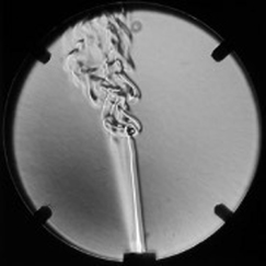
Figure 1. Schieren image of rising heated air from a candle.
Download figure:
Standard image High-resolution imageThe result of schlieren imaging is an image that at first glance looks a lot like a shadowgram and 'schlieren and shadowgraph methods are closely related' (Settles 2001, p 29). But unlike a shadowgram is schlieren image an optical image formed by a lens or something similar. To create this image you need a knife edge that cuts off the refracted light. The intensity of illumination of the image depends on the first spatial derivative of the refractive index and not on the second spatial derivative as it is the case with shadowgraphy. And most importantly, schlieren imaging has a higher sensitivity (Settles 2001).
2.2. Schlieren imaging of sound
The idea of using a schlieren system to make sound visible has existed almost as long as the idea of the schlieren setup itself. Toepler, also the name giver of this technique (Settles 2001), visualised a shock wave in 1866 (Korpel et al 1987). By then the observed shock wave was confused with actual sound (Hargather et al 2010). In 1935 developed Raman and Nathe a mathematical theory for the diffraction of light by high frequency soundwaves, describing the working principle of an acousto-optic modulator (AOM), by calculating that sound leads to a refractive index gradient that refracts light, which is also necessary to make ultrasound visible in a schlieren system (Raman and Nagendra Nathe 1935).
In 1976 did Bershader et al a calculation to see if airborne sound could be made visible using a schlieren setup (Bershader et al 1976). Using the following equations (2) and (3), they came to the conclusion, that a sound of f = 1000 Hz could not be made visible without exceeding the threshold of pain, with a sound pressure level of SPL = 82 dB (Bershader et al 1976):
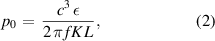
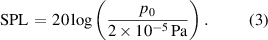
Using a sound pressure p0 defined by the speed of sound of c = 340 m s−1, K being the so-called 'Gladstone–Dale constant' (Bershader et al
1976, p 605), which is depending on the frequency of the light source but can be considered approximately constant, especially in this context, and is assumed for air with 2.3 × 10⁻⁴ m3 kg−1, L is the width of disturbance in direction of the optical axis and was chosen to be 0.1 m, and  the angular deflection (Bershader et al
1976). So unfortunately a schlieren setup cannot visualise audible sound (Crockett and Rueckner 2018). But using equations (2) and (3) one can easily see, that with increasing frequency the sound pressure level will drop accordingly. In 2010 Hargather et al came to the same conclusion, when they investigated the limits of such a setup. They reasoned that the refractive index gradient generated by the sound wave becomes larger with the increase of frequency of sound, when the acoustic power level is kept constant (Hargather et al
2010). This is also the reason why no audible sound is made visible in the setup presented here, but was limited to ultrasound. The first sound wave in air was made visible with a frequency between 200 and 20 kHz in 1977 by Bucaro and Dardy using schlieren technique (Bucaro and Dardy 1977). Since then, many of the components necessary for such a system have become more accessible to the general public, or there are inexpensive high-performance alternatives, such as LEDs. Crockett and Rueckner (2018) have also taken advantage of this in their setup, in which they were able to realise a simple schlieren setup for the visualisation of sound.
the angular deflection (Bershader et al
1976). So unfortunately a schlieren setup cannot visualise audible sound (Crockett and Rueckner 2018). But using equations (2) and (3) one can easily see, that with increasing frequency the sound pressure level will drop accordingly. In 2010 Hargather et al came to the same conclusion, when they investigated the limits of such a setup. They reasoned that the refractive index gradient generated by the sound wave becomes larger with the increase of frequency of sound, when the acoustic power level is kept constant (Hargather et al
2010). This is also the reason why no audible sound is made visible in the setup presented here, but was limited to ultrasound. The first sound wave in air was made visible with a frequency between 200 and 20 kHz in 1977 by Bucaro and Dardy using schlieren technique (Bucaro and Dardy 1977). Since then, many of the components necessary for such a system have become more accessible to the general public, or there are inexpensive high-performance alternatives, such as LEDs. Crockett and Rueckner (2018) have also taken advantage of this in their setup, in which they were able to realise a simple schlieren setup for the visualisation of sound.
2.3. A simple schlieren setup for school
Following the structure of Crockett and Rueckner (2018) a structure is now presented here which can also be realised outside of laboratories and especially with materials mostly found at school or at home. However, it is possible to approach this already quite simple structure in an even simpler and more rudimentary way, if the intention is to realise a simple experiment for school. Of course, this way one makes compromises in the quality of the pictures. This is especially noticeable on the photos. Live and in motion this experiment is very impressive, sample videos are available at: https://doi.org/10.25835/0040199.
A scheme of the single mirror off-axis schlieren system is shown in figure 2. The whole setup can be reproduced with relatively simple equipment, which is present in most of the physics and media collections in school, or they can be purchased at a reasonable price (a detailed list and explanations can be found in appendix
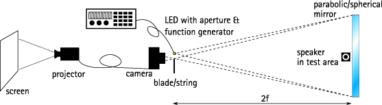
Figure 2. Scheme of the simple single mirror off-axis schlieren system. A detailed description of the particular components can be found in the appendix.
Download figure:
Standard image High-resolution imageIn principle the presented experiment is just a simple schlieren setup, which can also be used to visualise, e.g. the flow of cold or hot air (as can bee seen in figure 1). A detailed description of how this structure can be built up in steps is given in appendix
The heart of the structure is the concave mirror, which should have a long focal length, as this increases the sensitivity of the setup (Crockett and Rueckner 2018). Since the price for such a mirror increases significantly with the diameter, one has to consider how much needs to be displayed. For demonstration purposes it is nice if the length of one hand fits in front of the mirror. As a point light source a normal LED with high luminous intensity is used. It does not need to be a High Power LED as in the setup of Crockett and Rueckner (2018), even though the quality of the image would of course improve with a High Power LED and a diffuser. A normal LED covered with aluminium foil with a small hole punched into it works also fine enough. This is crucial because the tinier the light source is, the higher the sensitivity, because the deflection of the light will also be very small (Crockett and Rueckner 2018). But it should not be too small, because the image brightness should still be sufficient.
The sound source is taken from an experiment kit for schools. This has two advantages: it can be considered harmless for humans and it is immediately ready for use. With a frequency of 40 kHz, which corresponds to a wavelength of 0.86 cm in air, the pattern is big enough to be discernible (see figure 3).

Figure 3. Schlieren image of ultrasound emerging from the loudspeaker on the right. The left picture shows a single tone, and the right picture shows the interference pattern caused by sound coming out of two loudspeakers. Unfortunately, the pattern cannot be seen so well if the picture is printed out. A better impression is given in the videos, which can be found at the following address: https://doi.org/10.25835/0040199.
Download figure:
Standard image High-resolution image
To make this event, which is too fast for the human eye, perceptible, a very old but effective optical trick is used, stroboscopic illumination. To do this, the LED is connected to a function generator that pulses the LED at the frequency of the sound source. This optically stops the propagating density differences, which are due to the sound. By varying the pulse frequency of the light source and ,e.g. choose a slightly lower frequency, 1 or 2 Hz is enough, it will look like the sound wave is slowly moving forward. Of course this also works in the opposite direction, then the sound wave goes backwards, which is rather irritating.
With this structure an airborne sound wave was made visible. All in all, the structure described here can be implemented quickly and easily and is described in detail in appendix
3. Possible applications
The possibilities that this experimental setup offers are endless and here can only be given a small insight into them, examples can also be seen in the videos mentioned before. The biggest benefit of this experiment is the possibility for students to observe their own direct interaction with sound. And this is crucial for a good learning environment (Vosniadou 2002).
3.1. Application for older students
Especially for older students, this experiment offers a wide range of possible applications which, at least in Germany, can be justified by the curricular guidelines. Because there it is specified for the senior classes that vibrations and waves must be treated in the first year of the qualification phase (Frenzel et al 2017).
In this topic, properties such as the propagation and wavelength of harmonic waves can be characterised with the help of the experiment. With a transparent ruler, e.g. the wavelength could be measured directly on the mirror itself. Our measurement resulted in a wavelength of 0.82 ± 0.077 cm, which means that the theoretical wavelength of 0.86 cm is within the measuring range. Other properties of mechanical waves, such as reflection and diffraction, can also be observed well with this method. Especially since the sound is ultrasound and the wavelength is therefore a pleasantly small size, it is much easier than with audible sound. Reflection can be used, e.g. to examine different materials to see what they do with ultrasound and how sound can be reflected in general. The behaviour of sound behind a boundary can also be studied impressively. To achieve the best possible effect, it is advisable to fix the various boundary surfaces in such a way that no unnecessary movements interfere with the observations and the air heated by the hand does not disturb the image. It is also conceivable to consider interference effects with two sound sources (as shown in figure 3 on the right). Even standing waves can be demonstrated. Only the refraction would be more difficult to realise. Of course, longitudinal waves can be compared with transverse waves in an excellent way.
Another interesting aspect in the context of this setup is the relationship between pressure, density, refractive index and the resulting deflection (Snell's law) in this experiment. From this understanding it can be concluded that sound is a pressure wave.
3.2. Application for younger students
The schlieren setup offers the potential to deal with the topic of sound on different levels of experience even with younger children. Younger students can experience with the help of the structure that sound is a part of the air and not a thing that floats through it.
We tested the experiment in two different elementary schools and studied it there with different pairs of elementary school students, with an age between 8 and 10. And even though ultrasound cannot be heard by the students and therefore they lack this sensory experience they made the connection of sound and air.
We have gradually approached the experiment. We first showed that the setup makes it possible to see air. The children could observe their hand movements in front of the mirror on the screen. This also made it clear to them that the screen directly shows what happens in front of the mirror. The experiment therefore offers a good opportunity, especially for younger children, to learn about air and various properties and states of air. Only after that did we bring sound into the playing field. We tried to bypass the inaudibility of ultrasound with a bat model to establish a connection between ultrasound and audible sound, which worked for most of the children. Since the density changes caused by sound are much smaller than those caused by the heated air of a hand, we initially did not let the students near the mirror here. But this did not lessen their enthusiasm and fascination. But the connection to air was still given by their own previous interaction.
4. Conclusion
It could be shown that a schlieren experiment to visualise sound can be simplified, so that it can be set up and demonstrated with less material and without problems outside of laboratories, e.g. in elementary or secondary schools. This also reveals another important finding: this experiment is not only suitable for older students, but is also accessible to primary school students. It offers all age groups a starting point for a more realistic understanding of the physical properties of sound. Regardless of the age group with which the experiment is to be carried out, this structure makes it possible to emphasise the connection with the transport medium air and shows the wave character without unnecessarily strengthening the analogy to water waves. Together with the aesthetic appeal of this experiment, which easily fascinates students, this is an experiment that will enrich the physics classroom, as it can make sound visible in a very impressive way.
Acknowledgment
We would like to thank everyone who contributed to this schlieren project. In particular, we would like to thank C Schomaker, V Fontanella and the two involved elementary schools and teachers for their support, as well as the reviewers who improved the article with their helpful comments and the TIB for funding the open access of this article.
Supplementary materials
Three sample videos of the experiment and the setup can be downloaded at: https://doi.org/10.25835/0040199. They show the ultrasound wave with the frequency of 40 kHz coming from the speaker on the right, how the ultrasound of 40 kHz coming from the right being reflected, absorbed or deflected by an obstacle and two speakers showing an interference pattern and the third video shows a step by step description of how to proceed if you want to reproduce the schlieren setup.
Authors contributions
S V designed the experiment with some contributions of G F and conducted the surveys in the elementary schools. The theoretical background was discussed together. S V prepared the paper, with significant contributions from G F.
Ethical statement
The interviews with the children in this study were conducted in accordance with the ethics policy. The implementation of the study was previously approved by the Lower Saxony state school authority (reference H1Rb-81402-(03/2019)).
Appendix A.: Detailed description of assembling the structure
The following list is a step by step description of how to proceed if you want to reproduce the setup.
A.1. Light source—LED
- The point light source is placed at twice the distance of the focal length from the mirror.
- The easiest way to do this is to use a small mobile light and find the position where light source and its sharp image are at about the same distance and height. That is where the LED should be positioned.
- The LED is mounted on a tripod with a crank so that the position and angle can be readjusted more easily.
- The LED is pulsed by a function generator with the frequency of the sound.
- With a piece of cardboard the reflected image of the LED is checked for three things:
- The image should be at the same distance (2 f) as the LED. If not, this can be changed by varying the distance between LED and mirror a bit.
- The image should be at the same height as the LED. If not the height should be adjusted.
- The image should be evenly illuminated. If this is not the case, the LED should be readjusted by tilting it on the tripod.
- Now, the LED is covered with aluminium foil or pinhole with a small hole punched into it.
A.2. Camera
- Behind the now very small reflected light spot at height and distance of the LED but slightly displaced, you then place the camera.
- The camera has to be positioned in an angle and height, so that you can see the mirror completely illuminated.
- Here you also might have to adjust the exposure compensation.
- With a long-focal zoom lens you can zoom until the mirror fills the whole picture.
- For demonstration purpose the image of the camera can be transmitted on a screen (e.g. via a projector or computer).
A.3. Knife edge or wire
- Exactly where the small reflected point of the LED is visible, a wire or knife edge is positioned.
- The wire or knife edge should be set in a 45° angle and cut the light spot in half (for the knife edge) or cover most of the image, about 90%–95% (for the wire). In this way both the horizontal and the vertical refractive index differences are detected. By using a very thin wire (e.g. an e-tone guitar string), the positive and negative refractive index changes are also detected, which can improve the overall sensitivity of the setup (Crockett and Rueckner 2018).
- Now you can see that the image from the mirror has darkened considerably.
- Optimally, of course, a completely black background would be ideal, so that all stray light is blocked, but this is unrealistic and not necessary.
- In order to check if everything is correctly adjusted, it is recommended to place a burning candle in front of the mirror. This way you should be able to see the impressive streaks or schlieren that should be clearly visible due to the strong temperature differences. But also the slightly warmer air rising from a hand should be visible now.
A.4. Loudspeaker or ultrasonic source
- Now only the last step is missing, the ultrasound source has to be positioned in front of the mirror.
- The sound wave should be visible and depending on the chosen offset of the stroboscopic illumination standing still or moving back or forward.
Appendix B.: List of utilised components
In table B1 is a list of all materials used for the schlieren setup. It is likely that many components are already available in the physics collection of a school (e.g. function generator, ultrasound speaker and camera) and therefore do not have to be purchased especially for this setup. The materials presumably present are marked with *. The biggest expense is probably the mirror. Here you can possibly also find used or small mirrors, which are lower in price.
Table B1. On the left side are the components to be purchased for the schlieren system with the required specifications. On the right side of the table, the components used here are listed with the corresponding specifications and prices, even if many of them did not have to be purchased anew. The materials presumably present are marked with * and a second total price without these components is also shown.
| Component | Specifications | Estimated price | Used component | Specifications | Price |
|---|---|---|---|---|---|
| Mirror | Spherical/ parabolic | 40–600 € | Primary mirror of a Newton telescope | Parabolic | 500 € |
Focal length: 
|
 mm mm | ||||
| Diameter d: 100-400 mm | d = 300 mm | ||||
| LED | Luminous intensity:  mcd mcd | 1–8 € | Tru Components 1557 176 LED | I = 40 000 mcd | 1.50 € |
| Forward voltage: U = 3.1 V | |||||
| Current: I = 30 mA | |||||
| Camera* | Lens focal length  : 100-200 mm : 100-200 mm | 200–1000 € | Canon EOS Rebel T2i |
 : 18–135 mm : 18–135 mm | 250 € |
| Tripods* for LED & camera | 10–50 € | Bresser TR-672AN Traveler Stativ | 50 € | ||
| Function generator* | Signal frequency 
| 100–400 € | Rigol DG1022 |
 MHz MHz | 320.11 € |
Frequency resolution  Hz Hz | Δf = 1 µHz | ||||
| Signal shape: rectangular | |||||
| Wire* or | diameter d : 0.3–0.7 mm | 1–10 € | E-guitar string | d = 0.5 mm | 4 € |
| Knife edge* | Sharp edge | 1–10 € | Kitchen knife | 4 € | |
| Ultrasound speaker* | frequency fS: 25-50 kHz | 100–1000 € | School kit by 3B Scientific Physics: SEG Ultraschall | fS = 40 kHz | 614,04 € |
| Sound pressure level (SPL): 110 dB at 10 V | |||||
| Total costs: | 452–2668 € | Total costs: | 1739.65 € | ||
| Total costs*: | 41–608 € | Total costs*: | 501.50 € |
Biographies
Sonja Isabel Veith studied physics at Leibniz University Hannover and works there as a research assistant at the Institute for Special Education. Her work focuses on science and technology education. For her PhD, she is researching students' perceptions of sound.
Gunnar Friege has a degree in physics and both teacher degrees in physics and mathematics. He received his PhD at the University of Kiel in 2001. Since 2008 he has been a full professor of physics education at Leibniz Universität Hannover. Problem solving, multimedia, inquiry learning and informal learning are among his research interests.