


Abstract
We develop an ab initio time-dependent wavefunction based theory for the description of a many-body system of cold interacting bosons. Like the multi-configurational time-dependent Hartree method for bosons (MCTDHB), the theory is based on a configurational interaction Ansatz for the many-body wavefunction with time-dependent self-consistent-field orbitals. The theory generalizes the MCTDHB method by incorporating restrictions on the active space of the orbital excitations. The restrictions are specified based on the physical situation at hand. The equations of motion of this time-dependent restricted-active-space self-consistent-field (TD-RASSCF) theory are derived. The similarity between the formal development of the theory for bosons and fermions is discussed. The restrictions on the active space allow the theory to be evaluated under conditions where other wavefunction based methods due to exponential scaling in the numerical effort cannot, and to clearly identify the excitations that are important for an accurate description, significantly beyond the mean-field approach. For ground state calculations we find it to be important to allow a few particles to have the freedom to move in many orbitals, an insight facilitated by the flexibility of the restricted-active-space Ansatz. Moreover, we find that a high accuracy can be obtained by including only even excitations in the many-body self-consistent-field wavefunction. Time-dependent simulations of harmonically trapped bosons subject to a quenching of their noncontact interaction, show failure of the mean-field Gross-Pitaevskii approach within a fraction of a harmonic oscillation period. The TD-RASSCF theory remains accurate at much reduced computational cost compared to the MCTDHB method. Exploring the effect of changes of the restricted-active-space allows us to identify that even self-consistent-field excitations are mainly responsible for the accuracy of the method.
Export citation and abstract BibTeX RIS

Original content from this work may be used under the terms of the Creative Commons Attribution 3.0 licence. Any further distribution of this work must maintain attribution to the author(s) and the title of the work, journal citation and DOI.
1. Introduction
Since the first realizations of Bose–Einstein condensates (BEC) [1–3], the experimental and theoretical investigation of trapped cold atoms has attracted much attention. It is nowadays experimentally possible to design and control systems with a specific number of atoms [4–6] trapped in various potential shapes [7, 8] and dimensions [9], with tunable inter-particle interactions [10, 11], and to provide a controllable transition from a few- to a many-particle system. Such a detailed control of cold atom systems has opened the possibility to simulate various physical systems [12] from solid-state physics [13] to black-holes analogs [14] through matter–light interaction [15] and electrons dynamics in molecules [16].
Various theoretical models [17] have been used so far to describe static and dynamical properties of many-boson systems, among which, a handful are exactly solvable. One of the most prominent models was introduced by Lieb and Liniger [18, 19], to describe a system of spinless bosons interacting through a two-body contact interaction: using the Bethe Ansatz and periodic boundary conditions the resulting Schrödinger equation can be solved exactly for any interaction strength and an arbitrary number of bosons. Unfortunately, this model is exactly solvable only without a trapping potential. In one spatial dimension and in the limit of infinite interaction strength, the Tonks-Girardeau model use the Fermi-Bose mapping to map the wavefunction of bosons into a fermonic wavefunction of non-interacting fermions with frozen parallel spins [20]. This mapping provides the exact solution for the ground-state of the system for arbitrary trapping potentials and remains valid also for the excited states, as well as non-equilibrium solutions also for any external potential [21]. In the case of non-interacting bosons or more generally in the Gross-Pitaevskii (GP) limit, i.e.,  and
and  , with N the number of bosons and λ the interaction strength, the GP equation or its time-dependent (TD-GP) analog provides the exact description of the system. In this situation, the exact wavefunction of the system is described by a single product of single-particle functions and the interactions between the particles are correctly described by the mean-field approach. The above models assume that the bosons interact through a pair-wise contact potential. Considering other types of interaction potentials between the particles, other models can be solved exactly with an external potential. One model uses an inverse-harmonic interaction between the particles and can be solved exactly with a harmonic trapping potential [22], while an other model considers a harmonic interaction potential [23, 24]. The latter model has the peculiarity that it can be solved exactly numerically also for time-dependent Hamiltonians with a time-dependent trapping potential or a time-dependent interaction potential for bosons [25, 26] and fermions [27].
These exact models, unfortunately, do not cover the large variety of interaction or trapping potentials that are encountered in experiments. Nonetheless, they are of primary interest as they provide a unique way to benchmark numerical methods and approximations. The GP equation can be simplified when the potential and interaction energies are much larger than the kinetic energy, giving rise to the Thomas-Fermi approximation when the kinetic energy is neglected [28]. On an other hand, to overcome the lack of correlation in the GP theory and to take into account a small depletion of the BEC, i.e., to account for atoms which are not in the condensate, a perturbative expansion of the particle number in the condensate leads to Bogoliubov theory [29–31]. In the specific case of periodic trapping potentials, such as optical lattices [9], for weak contact interactions and deep lattices the Bose–Hubbard model (BHM) [32] is obtained by expanding the Bose field operator in term of the Wannier functions of the lowest Bloch band and neglecting the tunneling between nonconsecutive sites and interactions between different sites. The BHM and its various extensions have been extensively and successfully used to describe the ground state of trapped atoms in optical lattices and their dynamics [33]. A more general and efficient numerical approach than the BHM to deal with optical lattices is the density-matrix renormalization group method [34–36] based on the matrix product states Ansatz [37]. The method has been used to provide accurate results for ground and exited states of the system, and more recently has been used to investigate time-dependent systems [38–40]. The second wide-spread and promising numerical method to study trapped atoms is the quantum Monte Carlo (QMC) approach. It includes, among others, the variational Monte Carlo (VMC) [41] and the diffusion Monte Carlo (DMC) [42–45] methods, which used a Bijl-Jastrow decomposition of the wavefunction [46, 47], but are, however, not applicable to time-dependent systems.
Along with the above theory developments it has been a long standing idea to explore quantum chemistry methodologies to describe a time-independent system of trapped cold atoms. This idea was, to the best of our knowledge, introduced by the work of Esry [48], applying the mean-field Hartree–Fock (HF) theory and the configuration interaction (CI) method up to double excitations (CISD) to harmonically trapped bosons. The HF method for bosons can be viewed has a variant of the GP theory but has the advantage that it provides a set of optimized virtual orbitals, i.e., non-occupied orbitals, that can be subsequently used in a CI expansion of the wavefunction. The CI expansion corrects the lack of correlation between the particles, not included at the HF level. The CI method is in principle exact but requires a severe truncation of the CI expansion to be numerically tractable. Later, Streltsov et al [49] introduced the multiconfigurational Hartree theory for bosons (MCHB), which is an extension of the multiconfiguration self-consistent field (MCSCF) method introduced for fermions and widely used in electronic-structure calculations in atoms and molecules [50]. The MCHB method uses a CI expansion Ansatz for the many-body wavefunction in which both the coefficients of the expansion and the orbitals are variationally optimized, providing better accuracy with substantially less configurations and orbitals. The coupled-cluster (CC) method was originally introduced in nuclear physics [51, 52] and subsequently extended to describe electronic wavefunctions in atoms and molecules [53]. This framework was also extended to bosons up to double excitations (CCSD) by Cederbaum et al, and successfully applied to various particle numbers and interaction strengths [54].
Over the past decade, numerous numerical methods were developed [55–60] to tackle the problem of time-dependent multi-electron dynamics induced by laser pulses that are strong or short or both [61–63]. In short, the various successful methods used so far to investigate static properties of atoms and molecules have been extended to solve the time-dependent Schrödinger equation including a time-dependent operator. Among these methods, the multiconfigurational time-dependent Hartree–Fock method [64–67] variationally optimizes a set of time-dependent orbitals and CI coefficients, following the idea of the multi-configurational time-dependent Hartree (MCTDH) method [68, 69], originally introduced to describe molecular dynamics. The MCTDHF method was extended to identical bosons, within the framework of the MCTDH for bosons MCTDHB [70], in which the indistinguishability is taken into account using permanents instead of Slater determinants. Further developments include the case of particle mixtures of different type of bosons and fermions [71, 72], dynamics described by Hubbard Hamiltonians [73] and bosons with internal degrees of freedom [74]. The fundamental concept of using a set of time-dependent single-particle functions or orbitals to expand the total wavefunction offers the possibility to use substantially less orbitals than in the case of time-independent orbitals, because the former basis optimally adapts during the evolution of the system. Recently, the framework of the multi-layer (ML) MCTDH method [75–77] was extended to systems of bosons and mixtures of them [78, 79]. The method uses a ML expansion to reduce the size of the wavefunction in comparison to the MCTDHB method for multi-species or multi-dimensional systems. It is particularly effective for systems which can be subdivided in strongly interacting subsystems while the individual subsystems interact only weakly with each other. In the case of a one-dimensional system consisting of only a single type of particles, the ML-MCTDHB and MCTDHB wavefunctions are identical [80].
The MCTDHB method sheds new light on the dynamics of trapped cold atoms, especially when fragmentation occurs and more than one orbital is populated—a situation which cannot be described by the TD-GP theory. Fragmentation occurs in different systems such as during the dynamics at a Josephson junction [81], which is a universal phenomenon [82], and cannot be described, even qualitatively, using the TD-GP or BH theories. In double-well trapping potentials, fragmentation of the BEC is also obtained for the ground-state [83] for large barrier height between the two wells and the GP theory fails to describe the variance of position and momentum operators [84]. Multiconfigurational methods are also required to accurately describe the formation and dynamics of fragmented states with repulsive or attractive interactions between the particles [85–87] and tunneling of a many boson system to open space [88] or tunneling of trapped vortices [89]. Using time-dependent orbitals reduce the number of orbitals and thus the number of configurations required to describe accurately time-evolving systems in comparison with methods with time-independent orbitals. Nevertheless, simulations using such full-configurational wavefunctions remain a difficult task due to the exponential scaling of the configurational space, i.e., the dimensionality determined by the number of ways to arrange N particles in M orbitals, especially for bosons.
This challenge leads us to the quest for a theory which maintains the appealing properties of the time-dependent orbitals based methods mentioned above, but is free from the exponential scaling problem. One such theory uses the concept of a restricted active-space (RAS), well-known in quantum chemistry, where it was applied with time-independent molecular orbitals [90]. The RAS based method was successfully extended to time-dependent orbitals in the time-dependent RAS self-consistent-field method (TD-RASSCF) to deal with electron dynamics in atoms [91, 92]. Introducing a RAS scheme by fixing the promotion of the electrons between three sets of orbital spaces can considerably reduce the number of configurations. In addition, the theory includes, as limiting cases, the TD Hartree–Fock (HF), the TD complete active space self-consistent field (TD-CASSCF) [59] and the MCTDHF frameworks. Successful applications of the TD-RASSCF method include calculations of the ground-states (GS) of atoms, and time-dependent dynamics in the presence of strong laser fields to describe, for instance, high-order harmonic generation [91–93]. The aim of this work is to extend the TD-RASSCF theory to systems of spinless interacting bosons. To follow the generic naming introduced for the MCTDH methods, we call this method TD-RASSCF-B where the additional B stands for bosons and we will refer to the original TD-RASCSF method for fermions [91, 92, 94] as TD-RASSCF-F to avoid any confusion concerning the particles considered. We derive the working equations of the TD-RASSCF-B method and we present the general set of working equations for the TD-RASSCF method where the type of particles, i.e., bosons or fermions, plays a role in the symmetry of the creation and annihilation operators, only. The applications of the method to compute the GS energy of trapped bosons show that the TD-RASSCF-B theory provides very accurate results, in comparison to MCTDHB, while the expansion of the wavefunction is considerably reduced. Moreover, the MCTDHB accuracy can be overtaken by using large numbers of time-dependent orbitals while the number of configurations remains small thanks to the considered RAS. The TD-RASSCF-B theory can be evaluated in situations where other accurate wavefunction based methods cannot. In addition, and very importantly, the theory allows an identification of the types of excitations that are important in obtaining accuracy. For the GS calculations, it is hence important to allow a few particles to move in many orbitals, representing physically a situation where a small number of particles are outside the condensate, but move relatively fast. For the GS we find that accurate results can also be obtained by including only even excitations in the RAS scheme. Insights, that may seem natural, and are now supported by ab initio theory. The investigation of the breathing dynamic of a BEC confined to a harmonic trap illustrates how the TD-GP theory fails to describe the time-evolution of the system within a fraction of a harmonic oscillation period, while various examples of the TD-RASSCF-B method either qualitatively or quantitatively reproduce the exact dynamics obtained using the MCTDHB method, depending of the choice of the excitation scheme. In particular, we find that very accurate results can be obtained retaining only even excitations in the RAS scheme, again an example of physics insight obtained by the flexibility of the TD-RASSCF-B theory.
The paper is organized as follows. In section 2.1 we introduce the TD-RASSCF-B Ansatz for the wavefunction and in section 2.2 we derive the equations of motion for the set of coefficients and orbitals, and highlight the similarity of the formulation for bosons and fermions. In section 3 the method is applied and compared to the MCTDHB method to study the static properties of a system consisting of N = 100 bosons trapped in a harmonic potential. The applicability of the method to time-dependent systems is illustrated by two examples of breathing dynamics following a sudden quench of the two-body interaction in section 4. Finally, in section 5 we conclude and provide perspectives to future work. In the appendices
2. Theoretical framework
2.1. Ansatz for the many-body wavefunction
For the energy regime of interest, the time evolution of a system composed of N bosons is governed by the time-dependent Schrödinger equation:

with  the many-body Hamiltonian of the system and
  the N-particle wavefunction. Hereafter we set
  , unless explicitly specified. We can approximate the wavefunction using linear combinations of suitably symmetrized sets of products of time-dependent single-particle functions
  . In the following, the single-particle functions are denoted orbitals. To take into account the indistinguishability of the bosons, the total wavefunction is expressed in terms of permanents. For a given number of bosons and orbitals the multi-configurational wavefunction is constructed by taking into account all the possible arrangement of the particles in the given orbitals, each arrangement being called a configuration
  ,
,

This Ansatz converges to the exact wavefunction when the number of orbitals increases to infinity. The configurational space, i.e., the number of coefficients  , increases exponentially with respect to the number of orbitals and often makes a numerical treatment impossible, even for a small number of orbitals. In the case of a system of N bosons and M orbitals, the dimension of the full-configurational Fock space
  can be evaluated as,

In the case of the TD-RASSCF-B method, we introduce two orbital spaces,  and
and  , such that
  , with M1 and M2 the number of orbitals in
  and
and  , respectively (see figure 1). The
  subspace must include enough orbitals such that it can accommodate all the particles. For bosons one orbital, i.e.,
  is the lower bound, and there is no restriction concerning the upper bound. In this subspace all the configurations are used to construct the total wavefunction. Concerning the
  -space, particles are promoted from
  to
to  according to a specific excitation scheme, which restricts the maximal number of particles promoted from
  to
to  . This number is chosen at will and the restriction of the configurational space provides a way to constrain its size, defining the Ansatz for the TD-RASSCF method as,

where the configurations are drawn from the space  subject to restrictions. To evaluate the size of the space
  , we introduce
  the highest number of bosons in
  and consider a RAS scheme allowing all occupations of
  from 0 to
  . The dimension of the space
  of equation (4), is then given by

Here, the first term is the total number of configurations obtained with the N bosons in the M1 orbitals and no particle in  . The second term in equation (5) takes into account the configurations resulting from the excitation of k bosons in
  , with
  . The total number of configurations with k bosons in
  is obtained as a product of the possible arrangements of k bosons in M2 orbitals and
  bosons in M1 orbitals, see also appendix
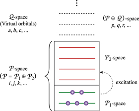
Figure 1. Division of the single-particle Hilbert space within the TD-RASSCF-B framework. The  -space orbitals, used to expand the wavefunction, are divided in a
  and
and  space between which the particles can be excited through a specific scheme chosen at will. The orthogonal complement of virtual (i.e., unoccupied) orbitals is referred to as the
  -space. The indexes
  are used to label the orbitals of the
  -space, the indexes
  to label the orbitals of the
  -space and the indexes
  are used for orbitals in either the
  - or
- or  -space.
Download figure:
Standard image High-resolution imageThe TD-RASSCF-B Ansatz has some interesting properties. First, if only  orbitals are used, i.e.,
  and
and  , then the TD-RASSCF-B and MCTDHB Ansätze are equivalent with the same number of configurations, as seen be replacing M1 by M in equation (5). Note that this is also true for
  and
and  . Moreover, if only a single time-dependent orbital is considered, i.e.,
  and
and  , the RAS wavefunction includes a single configuration with all particles in one orbital, which is equivalent to the time-dependent GP wavefunction. Thus the theoretical framework of TD-RASSCF-B is very general and holds, as limiting cases, the GP and MCTDHB theories. The TD-RASSCF-B wavefunction is built from a set of time-dependent coefficients
  and orbitals
  . To describe its dynamics, we need a set of equations of motion (EOM), which provides the time-evolution of the coefficients and orbitals through their time-derivatives
  and
and  . The
. The  -space is a subset of the total single-particle Hilbert space and we can define its orthogonal complement,
  , collecting the virtual orbitals, as depicted in figure 1. While in the case of time-independent orbitals these two subspaces remain fixed, in the case of time-dependent orbitals the
  -space is variationally optimized at each time and both
  - and
- and  -space are time-dependent. We can define
  and
and  , the time-dependent projectors onto the subspaces
  and
and  , respectively, with the property
  , the identity operator. The role of the
  -space emanates from the time-derivative of the
  -space orbitals, that can be written as,

with one contribution from the  -space and one contribution from the
  -space. In the following we establish the EOM of the TD-RASSCF-B theory, providing the time-derivative of the expansion coefficients in section 2.2.1 and the time-derivative of the orbitals (section 2.2.2) through the
  - and
- and  -space contributions given in sections 2.2.2.1 and 2.2.2.2, respectively.
2.2. Derivation of the working equations
The EOM for the TD-RASSCF-F theory have been already established in [91, 92]. In the following we provide the derivation of the EOM in the case of the TD-RASSCF-B method, and highlight the similarities and differences with respect to the TD-RASSCF-F theory. Starting from the Lagrangian formulation of the time-dependent Schrödinger equation [95], we define the action functional using the TD-RASSCF-B Ansatz, equation (4), as,

with  and
and  the Kronecker delta function. The Lagrange multipliers,
  , ensure that the orbitals remain orthonormal for all time t. In the following the indexes
  are used to denote the orbitals of the
  -space, the indexes
  denote the orbitals of the
  -space and
  are used for either
  - or
- or  -space orbitals, see also figure 1. For our purpose, we consider only one- and two-body operators, such that the Hamiltonian can be expressed in the framework of second quantization as

with  (
( ) the annihilation (creation) operator of a particle in the orbital
  (see also appendix
 ![$[{\hat{b}}_{p},{\hat{b}}_{q}^{\dagger }]={\hat{b}}_{p}{\hat{b}}_{q}^{\dagger }-{\hat{b}}_{q}^{\dagger }{\hat{b}}_{p}={\delta }_{{qp}}$](https://content.cld.iop.org/journals/1367-2630/19/4/043007/revision1/njpaa6319ieqn85.gif) , for bosons and the anti-commutation relation,
, for bosons and the anti-commutation relation,  , for fermions, see for instance [96]. The matrix elements of the one-body and two-body operators in the basis of the time-dependent orbitals, are expressed as

and

respectively. In the following, the explicit time dependence of the operators, coefficients and orbitals is dropped for brevity.
According to the time-dependent variational principle [95, 97], the best approximation using the wavefunction Ansatz is obtained by seeking stationarity of the action S, i.e.,  , for any variation of the parameters and with the boundary condition
  . The variation of the action gives,

where the boundary condition is used to remove the additional term  resulting from the action of
  on
on  instead of
  , see [97]. The variation of the wavefuntion is explicitly written as [91],

We can now proceed with the stationarity condition of the action with respect to the parameters  ,
,  and
and  to obtain the EOM of the TD-RASSCF-B method.
2.2.1. Equations of motion for the coefficients
The variation w.r.t the Lagrange multipliers leads to the conservation of the orthonormality of the orbitals. We then consider the variation of the action functional with respect to the expansion coefficients. The action S depends on the expansion coefficient  only through the bra
  of the first expectation value in equation (11). Thus, the stationarity condition,
  , readily leads to
  . Moreover, the derivative of the wavefunction with respect to time reads,

with  , which results from the time-derivative of the orbitals used to build the configurations in
  . Hereafter, the operator in bracket in equation (13) will be called
  , i.e.,

for brevity. We can now rewrite the stationary condition  using the explicit form of
  , equation (13), as

or equivalently, using the expressions of  and
and  ,
,

The indexes in the summations are now restricted to the  -space. It is clear that if either annihilation or creation operators act on an orbital of
  , the inner product with all RAS configurations
  vanishes. The EOM for the expansion coefficients, the amplitude equation (16), are identical to those obtained for fermions in the TD-RASSCF-F theory, see [91, 92], and those of the MCTDHB [70] and MCTDHF [98] theories. It is worthwhile to keep in mind that the action of the creation and annihilation operators differs for fermions and bosons. The
  matrix elements in the amplitude equations (equation (16)) describe the rotation of the orbitals into one another and are also present in the EOM of the MCTDHB/F methods. In these latter cases, besides to be elements of an anti-Hermitian matrix, there are no constraints on the
  and their values are usually set to zero. The same is true in the TD-RASSCF-B/F methods for equivalent orbitals, i.e., for pairs of orbitals which belong to the same
  -space (i = 1, 2). For orbitals which do not belong to the same
  -space, the
  matrix elements must be evaluated, as discussed in [91, 92] and in sections 2.2.2.3 and 2.2.2.4.
2.2.2. Equations of motion for the orbitals
Seeking stationarity of S with respect to a variation of an orbital  , i.e.,
  , gives

with  . The index q in the above equation runs over all the orbitals, i.e., the orbitals of the
  -space and the
  -space, see figure 1. The EOM for the orbitals of the
  - and
- and  -space are obtained by projecting equation (17) on either an orbital of the
  -space,
  , or of the
  -space,
  , as done in the following.
2.2.2.1. Equations of motion for the  -space orbitals

Starting with the EOM for the  -space orbitals, we multiply equation (17) from the left with an orbital
  belonging to the
  -space and obtain,

where we used the orthogonality between the orbitals of the  and
and  spaces to get rid of the Lagrange multipliers. Moreover the inner product
  vanishes because in all configurations
  the orbital
  is unoccupied. Using the explicit expression of the Hamiltonian, equation (8), and for the operator
  , equation (13), we obtain

Using the commutation relation for the creation/annihilation operators for bosons (fermions), we can reestablish the normal ordering of the chains of operators,


with the upper sign holding for bosons and the lower for fermions. The chain of four operators in equation (20) and six operators in equation (21) both annihilate a particle in orbital  , from the
  -space, which is not included in
  and thus vanish. The lhs of equation (19) now reads,

where we restrict the summation over  , the summation over the
  -space orbitals being zero. In the same way, inserting equation (21) in the rhs of equation (19) simplifies its expression to

Here we used that  (equation (10)). Interestingly, this equation is exactly the same for bosons and fermions. The time-derivative of the orbitals, included in the term
  , requires the explicit consideration of the
  -space orbitals. This issue is circumvented by using the projector
  onto the subspace spanned by the
  -space orbitals,

with  the projector onto the
  -space. Introducing the one-body density matrix,
  and the two-body density matrix
  , we obtain,

with,

the mean-field operator, which describes the interaction between the particles and h the one-body Hamiltonian from the rhs of equation (9). The role of the  -space appears in the time-derivative of the orbitals of the
  -space through the term
  , see equation (6). We rearrange equation (25), see appendix
  , and obtain

with  the inverse of the one-body density matrix. The MCTHB theory leads also to equation (27), see [70], but the lhs is subsequently simplified thanks to the choice of the matrix elements
  and using
  , see equation (31) below. As discussed in 2.2.1, such a fixed choice of
  is not possible in the TD-RASSCF theory. The derivations of the
  -space EOMs differ slightly for bosons and fermions, see equations (20) and (21), but the final result, equation (27), is the same for both types of particles.
2.2.2.2. Equations of motion for the -space orbitals

Going back to the stationary condition for the variation of the action functional with respect to an orbital, equation (17), we multiply this latter on the left by an orbital of the  -space,
  , leading to,

with  defined in equation (14). This equation still contains the Lagrange multiplier
  . A variation of S with respect to the orbital
  and its projection onto the orbital
  , leads to an equation containing the same Lagrange multiplier,

and subtracting equations (28) and (29) gives the EOM for the  -space orbitals, i.e.,

where we have introduced  , with
  . The
. The  -space EOM provide the contribution of the
  -space in the time-derivative of the orbitals, see equation (6),

through the evaluation of the matrix elements  included in the operator
  , see equation (14). Nonetheless, solving equation (30) is not a trivial task because of the presence of
  , which couples the amplitude and
  -space orbitals equations. In the case of the wavefunction based on the RAS Ansatz, a freedom in the choice of the elements
  is still possible for pairs of orbitals which belong to the same
  -space (i = 1, 2), and we use
  . The
. The  -space equation (equation (30)) remains to be solved only for pairs of orbitals
  , which belong to different
  -spaces,

but remains coupled to the amplitude equations through  . In the meantime it is noted that if equation (32) is solved for
  , the rhs of equation (31) can be constructed. Moreover equation (27) can be solved, and hence
  of equation (6) can be evaluated. In the derivation of the TD-RASSCF-F method [91, 92], two different approaches of RAS schemes were proposed to circumvent the difficulty of solving equation (30). These approaches are also used for bosons in the following sections (2.2.2.3) and (2.2.2.4).
2.2.2.3. Even excitation RAS scheme
First we suggest to consider the case in which only an even number of particles is promoted from  to
to  , see figure 2(a). In this case,
  explicitly reads,

The action of  on the wavefunction
  annihilates one particle in
  and creates one in
  . Since only an even number of particles is present in
  ,
,  would contain only configurations with an odd number of particles in
  , which makes the inner product with
  vanish. In the same manner
  acting on
  is either zero, if
  is unoccupied in the configuration
  , or gives an odd number of particles in
  . In this specific excitation scheme,
  , for all pairs of orbitals
  , leaving the amplitudes and the
  -space orbitals equations uncoupled. Using the explicit expressions of the Hamiltonian (equation (8)) and the operator
  (equation (14)), equation (32) reads,

We can simplify this expression, starting with

Now we turn to the chains of six operators in the last term in equation (34). The first product of operators is expressed as

and the second product of operators as

The sum of equations (36) and (37) enters equation (34), and we see that the chains of six operators cancel each other and only the chains of four operators remain. Using the fact that  (equation (10)) and that
  must be evaluated for orbitals which belong to different
  space,
  , equation (34) can be rewritten,

This equation, used to determine  , is identical for fermions and bosons, only the evaluation of the one- and two-body reduced density matrices depends on the kind of particles. The coefficients and the
  -space orbitals equations are separable and can now be solved (see appendix
  , obtained from equation (38), are used to determine the time-derivative of the coefficients from equation (16). The time-derivative of the
  -space orbitals, equation (6), is obtained from equation (31) in addition to the
  -space equations (equation (27)). Interestingly, for the case of only even excitations where
  , equation (30) is the analog of the generalized Brillouin's theorem, or Levy-Berthier-Brillouin theorem [99, 100], for the time-dependent Schrödinger equation with
  . It means that the single excitations of the wavefunction, i.e.,
  , are not coupled to the wavefunction
  through the action of
  ,
,  . Thus, the TD-RASSCF-B wavefunction with only even excitations always includes the subspace of single excitations, see also [59, 91]. In other words, projecting the TD-RASSCF-B wavefunction onto a time-independent basis would include non-vanishing projection in the singles space spanned by the time-independent basis functions.

Figure 2. Illustration of the decomposition of the Fock-space used in the TD-RASSCF-B method with N = 8 bosons, a single  orbital,
  (thick (green) line) and
 orbitals (thin (red) lines). (a) For a RAS scheme including only even excitations, the RAS Fock-space
  is decomposed into the direct sum of subspaces
  with
with  . Each subspace
  includes all the configurations with n bosons in
  and N − n bosons in
  . (b) The decomposition of the RAS Fock-space for the general excitation scheme is also written as a direct sum of subspaces
  except that in that case
  .
.
Download figure:
Standard image High-resolution image2.2.2.4. General RAS scheme
Considering only even excitations provides an efficient and simple way to uncouple the equations of the TD-RASSCF-B method. Nonetheless, it is also possible to consider both even and odd excitations in the configurational space. In the following, we specifically consider a RAS scheme with all successive numbers of particles occupying  from 0 to
  , where
  , defined in section 2.1, is the highest number of particles allowed in
  , see figure 2(b). Note that
  must fulfill the condition
  . For instance, taking
  , we consider the promotion of 0, 1, 2, 3 and 4 particles from
  to
to  . In this way, the configurational space is the direct sum of
  subspaces,

Using the expression of the time derivative of the  coefficients, equation (15), the time derivative of the one-body density matrix, in equation (30), can be expressed as,

We introduce the projector onto the RAS space  as
as  . Using the above expression of
  , we obtain a new formulation of the
  -space orbital equation,

For  and
and  , we note that
  belongs to
  , with one particle from
  being annihilated and one particle in
  created, leading to
  . On the other hand,
  , provides configurations with a creation of an additional particle in
  , which may lie in
  , not included in
  . In this case,
  and equation (41) simplifies to,

Using the expression of the Hamiltonian (equation (8)) and of the operator  (equation (14)) while keeping in mind that
  has only to be determined for pairs of orbitals
  which belong to different
  subspaces, equation (42) is equivalent to

where the fourth- and sixth-order tensors are defined by


Here again, the  -space EOM for the determination of the
  , equation (43), are identical for bosons and fermions [91, 92]. These equations are solved to determine the
  for each pairs of orbitals belonging to different
  -spaces. The value of
  is subsequently used to solve the amplitudes equations (equation (16)) and to evaluate the time-derivative of the
  -space orbitals from equations (31) and (27), as for the case of the even excitation scheme.
The general excitations scheme and the only even excitations schemes were originally introduced in the case of fermions in [91, 92]. We mention that recently Haxton et al [93] derived a general RAS scheme for fermions, in the sense that the configurational space can be build from of any arbitrary configurations. For both excitation schemes presented in this work, the time-derivative of the coefficients and orbitals are obtained by solving the amplitudes equations, equation (16), the  -space equations, equation (27) and the
  -space equations equation (43) and equation (38) for the general RAS scheme and the only even excitation scheme, respectively. In the case of the MCTDHB method, the amplitude (equation (16)) and the
  -space equations (equation (27)) are also solved to obtain the time-derivative of the wavefunction, see appendix
  -space equations (equation (38) or (43)). For only even excitations, the number of operations required to obtain the time-derivative of the wavefunction is always smaller in the case of the TD-RASSCF-B method than in the MCTDHB method. In the case of the general excitation scheme, the evaluation of the sixth-order tensor, equation (45), requires a significantly large number of operations. Thus, the TD-RASSCF-B method may require more operations than MCTDHB for large values of
  and large numbers of orbitals. As shown in appendix
  , for instance for
  with N = 50 or
  for N = 1000 bosons. Except for these high excitation schemes, the TD-RASSCF-B method is numerically more efficient than the MCTDHB method, but more importantly the exponential grows of the configurational space with respect to the number of orbitals can be controlled thanks to the RAS Ansatz. In addition, we have shown that the TD-RASSCF equations of motion are the same for bosons and fermions, which means that the TD-RASSCF theory is a general framework including as limiting cases the TD-GP (TD-HF) and the MCTDHB (MCTDHF) theories for bosons (fermions). This result is reminiscent to the work of Alon et al [101] where a unified set of EOM for the MCTDH theory for both bosons and fermions was derived.
3. Application to a time-independent system: ground state energy
In this section, we consider a system of N = 100 bosons trapped in a one-dimensional (1D) harmonic potential. Experimentally, quasi-1D systems have been obtained by using a tight confinement in the transversal coordinates, freezing in that way the transversal dynamics of the system [102–106]. In the following, we consider an anisotropic harmonic trap such that the longitudinal frequency ( ) is much smaller than the transversal frequency (
 ), i.e.,
  , such that the transverse part of the wavefunction can be assumed to be energetically frozen to the ground state and be integrated out. The resulting 1D Hamiltonian for the N boson system reads,

using the unit of length  and the unit of energy
  , with m the mass of the particles. Assuming no confinement induced resonances [107], the interaction strength, λ, is related to the 3D s-wave scattering length of the particles, as, through
  , with l⊥ the transversal harmonic oscillator length. Experimentally, the 1D interaction strength can be tuned either by controlling the longitudinal and transversal frequencies or using an external magnetic field [10, 11]. The different parameters used to perform the numerical calculations are reported in appendix
To assess the accuracy of the GP, MCTDHB and TD-RASSCF-B methods we compare the GS energies and by virtue of the variational principle (see for instance [108]), the lower the energy, the higher the accuracy. First, as a general remark, for any value of  the energy obtained with the MCTDHB method systematically decreases with increasing number of orbitals and subsequently for increasing number of configurations, see for instance the first line of table 1 where the numbers of configurations are indicated in parentheses. Concerning the TD-RASSCF-B method, for a given excitation scheme the energy also decreases when the number of orbitals is increased. In addition, for a given number of orbitals the energy decreases when we increase the highest number of allowed particles in
  ,
,  . To simplify the following discussion, we introduce some quantities to help the comparison between the MCTDHB and TD-RASSCF-B methods. Firstly, we define the correlation energy as the difference between the energy obtained with a given method and the mean-field GP energy,

where  designates the energy obtained with a given method. By definition, the GP correlation energy is equal to zero and is considered as uncorrelated. We use as a reference,
  , the correlation energy obtained for the MCTDHB method with 5 orbitals, i.e.,

where the superscript 5 denotes the number of orbitals. Using this reference, we can easily compare the results obtained for different numbers of orbitals by expressing the correlation energy in percent of  . Secondly, we define the relative correlation energy,
  , as the difference between the energy obtained from a MCTDHB calculation with X orbitals and the GP energy, i.e.,

This quantity is particularly useful to compare the results of different RAS schemes within a given number of orbitals. Indeed, the TD-RASSCF-B Ansatz, with restrictions on the active space, is an approximation to the MCTDHB wavefunction. Thus, when the correlation energy of a RAS scheme with X orbitals is equal to  the calculation is converged.
Table 1.
Ground-state energy (in units of E0, see text after equation (46)) of 100 bosons trapped in a 1D harmonic potential interacting through a contact potential with a strength  . The TD-RASSCF-B calculations were performed with a single
  orbital,
  and
and 
 orbitals, with M the total number of orbitals. The results were obtained using either the general RAS scheme, labeled 'All excitations', or only even excitations, labeled 'Even excitations'. The excitation schemes are indicated with the usual notations -S, -SD, ..., up to
  and the RAS schemes are labeled by the value of
  for larger excitations, e.g. -10. In addition MCTDHB calculations were carried out to compare the accuracy and efficiency of the TD-RASSCF-B method. The number of configurations used in the wavefunction expansion are indicated in parentheses under each energy. The result obtained with a single orbital is equivalent to the GP method. To highlight the difference between the TD-RASSCF-B and MCTDHB results, the digits that differ are underlined.
| Orbitals | ||||||||
|---|---|---|---|---|---|---|---|---|
| Method | 1 | 2 | 3 | 4 | 5 | 6 | 7 | 8 |
| All excitations | ||||||||
| MCTDHB | 68.76816487 | 68.75335446 | 68.74538390 | 68.74152088 | 68.73891122 | — | — | — |
| (1) | (101) | (5151) | (176851) | (4598126) | (96560646) | (1705904746) | (26075972546) | |
| -SD | — | 68.75355024 | 68.74565678 | 68.74184781 | 68.73926413 | 68.73761231 | 68.736360917 | 68.73545355 |
| (3) | (6) | (10) | (15) | (21) | (28) | (36) | ||
| -SDTQ | — | 68.75335660 | 68.74538672 | 68.74152449 | 68.73891508 | 68.73724366 | 68.73598073 | 68.73506372 |
| (5) | (15) | (35) | (70) | (126) | (210) | (330) | ||
| -SDTQ56 | — | 68.75335448 | 68.74538393 | 68.74152092 | 68.73891126 | 68.73723959 | 68.73597655 | 68.73505943 |
| (7) | (28) | (84) | (210) | (462) | (924) | (1716) | ||
| -SDTQ5678 | — | 68.75335446 | 68.74538390 | 68.74152088 | 68.73891122 | 68.73723955 | 68.73597651 | 68.73505938 |
| (9) | (45) | (165) | (495) | (1287) | (3003) | (6435) | ||
| -10 | — | 68.75335446 | 68.74538390 | 68.74152088 | 68.73891122 | 68.73723955 | 68.73597651 | 68.73505938 |
| (11) | (66) | (286) | (1001) | (3003) | (8008) | (19448) | ||
| Even excitations | ||||||||
| -D | — | 68.75355024 | 68.74565780 | 68.74184905 | 68.7392653 | 68.73761353 | 68.73636218 | 68.73545481 |
| (2) | (4) | (7) | (11) | (16) | (22) | (29) | ||
| -DQ | — | 68.75335660 | 68.74538974 | 68.74153257 | 68.73892541 | 68.73725598 | 68.73599408 | 68.73507803 |
| (3) | (9) | (22) | (46) | (86) | (148) | (239) | ||
| -DQ6 | — | 68.75335448 | 68.74538700 | 68.74152917 | 68.73892180 | 68.73725217 | 68.73599018 | 68.73507404 |
| (4) | (16) | (50) | (130) | (296) | (610) | (1163) | ||
| -DQ68 | — | 68.75335446 | 68.74538697 | 68.74152914 | 68.73892177 | 68.73725213 | 68.73599014 | 68.73507400 |
| (5) | (25) | (95) | (295) | (791) | (1897) | (4166) | ||
| -10 | — | 68.75335446 | 68.74538697 | 68.74152914 | 68.73892177 | 68.73725213 | 68.73599014 | 68.73507400 |
| (6) | (36) | (161) | (581) | (1792) | (4900) | (12174) | ||
In table 1, we report the results for the GS energy (in units of E0) obtained with  . The reference for the correlation energy is
  (the GP result is obtained from MCTDHB with a single orbital). Increasing the number of orbitals in the MCTDHB calculations from 2 to 5 allows us to account for more and more of
  . Specifically we obtain 51%, 78% and 91% of
  for 2, 3, and 4 orbitals, respectively. The
  variation of the correlation energy between 4 and 5 orbitals indicates that the results are not fully converged with respect to the number of orbitals, and more than 5 orbitals are required to converge the energy below 10−3, see table 1. Unfortunately, the MCTDHB wavefunction with 5 orbitals includes already
  configurations and using 6 (8) orbitals leads to
  (
( ) configurations, far beyond the scope of any practical numerical implementation.
The TD-RASSCF-B method provides more flexibility to describe the wavefunction in the sense that we can choose different RAS schemes, different numbers of orbitals and their partitions into  and
and  spaces. In table 1 we report the results obtained for M = 2 to 8 orbitals with a single
  orbital, i.e.,
  and
and 
 orbitals, and a few specific cases of the general RAS scheme. We indicate the excitation schemes with the usual notation. For example -SD denotes that single and double excitations are allowed from
  to
to  . We follow this notation up to -SDTQ56789 and for larger excitations, we just indicate the value of
  (e.g., ''-10'' means that all excitations from
  to
to  up to 10 are included). For each number of orbitals, when we increase the excitation scheme the energy becomes closer to the MCTDHB result and converges to this latter for the -SDTQ5678 RAS scheme, as indicated by the underlined digits in table 1. Thus,
  is recovered for the -SDTQ5678 scheme with 5 orbitals, but the expansion of the wavefunction includes only 495 configurations, i.e.,
  times fewer configurations than the MCTDHB expansion for 5 orbitals. It is worthwhile to note that this RAS scheme converged for all number of orbitals, and always for much fewer configurations than with the MCTDHB. The least accurate TD-RASSCF-B calculation, presented in table 1, consists of 2 orbitals and the -SD RAS scheme. The correlation energy includes
  of
of  and interestingly when we increase the number of orbitals from 3 to 5, a similar amount of correlation is obtained (
 for all values) in comparison to the respective
  correlation energies. Thus, using the -SD scheme with 5 orbitals
  of
of  is obtained but the TD-RASSCF-B wavefunction includes only 15 configurations while the MCTDHB wavefunction includes more than
  configurations, i.e.,
  times more configurations. Moreover, the energy difference between the -SD scheme and the MCDTHB method is below
  , i.e., systematically lower than the convergence obtained with respect to the number of orbitals. Concerning the correlation energy of the -SDTQ and -SDTQ56 schemes, we find that they include
  and
and  of
of  , with X = 2 to 5. It is remarkable that the correlation energy remains almost constant while the difference between the number of configurations between the MCTDHB and TD-RASSCF-B increases exponentially with the number of orbitals. These results show that the correlation energy does not strongly depend on the number of configurations used in the wavefunction expansion, as the configurational space of the -SD RAS scheme increases only from 3 to 15 configurations for M = 2 to M = 5 but captures
  of
of  , with X = 2 to 5. Thus, the correlation depends more critically on the number of orbitals than the number of configurations used in the calculation. To illustrate this point, we compute the GS energy with 6 to 8 orbitals with the TD-RASSCF-B method, see table 1, and we obtain energies lower than the energy of the MCTDHB with 5 orbitals for all excitation schemes used here. It means that the -SD scheme with 8 orbitals and 36 configurations is more accurate than the MCTDHB method with 5 orbitals and
  configurations. Moreover, comparing the energies obtained for the -SDTQ5678 and -10 excitation schemes, we can conclude that the GS energy has converged with respect to the number of excitations. Thus, the TD-RASSCF-B method, thanks to the restriction imposed on the configurational space, can provide more accurate results than the MCTDHB method, whoes practical applicability is limited by the exponential growth of the number of configurations.
We also consider RAS schemes with only even excitations (see table 1), for which the numerical effort is always reduced in comparison to the MCTDHB method, see appendix  for all numbers of orbitals, indicating that more than
  of the relative correlation energy is obtained with slightly fewer configurations. The same conclusion holds for the comparison of the -DQ and -SDTQ schemes with an energy difference below
  , including more than
  of the relative correlation energy. The number of configurations is slightly smaller in the case of the RAS schemes with only even excitations but the numerical efficiency is better since the
  -space EOM, equation (38), does not require the update of a sixth-order tensor at each time-step as it is the case for the general RAS schemes, see equation (45). For values of
  and
and  , the energy converges with respect to
  , as the energy does not change by increasing
  further, but with energy slightly larger than the MCTDHB ones. The energy difference between the -DQ68 scheme and the MCTDHB calculation, with 5 orbitals for both methods, is
  and includes
  of
of  . In the case of only even excitations, we also find that for
  the energy for all schemes is below the energy of the best MCTDHB calculation performed. The comparison of the converged -DQ68 and -SDTQ5678 RAS schemes, show that the energy difference remains below
  for
for  , which is two orders of magnitude smaller than the convergence obtained with respect to the number orbitals,
  .
.
These preceding examples show that the TD-RASSCF-B method provides an efficient approach for computing the GS energy of trapped cold atoms. This wavefunction based approach gives access to quantities of interest such as the one and two-body reduced densities and the fragmentation using the analysis of the natural occupations of the natural orbitals [109]. The accuracy was compared with the MCTDHB results and we showed that the TD-RASSCF-B method converges for relatively low excitation schemes. Moreover, the possibility to constrain the growth of the configurational space gives the possibility to use more orbitals than in the MCTDHB calculations and better results (lower energies) were systematically obtained using the TD-RASSCF-B method. This result can be understood as follows. The MCTDHB wavefunction for a small number of orbitals generates a large number of configurations, as all orbitals can be equally populated. Most of these configurations, however, do not contribute in lowering the energy of the system as they describe states with many particles occupying the same spatial orbital, which induced a large interaction energy for a large value of λ. As a limiting case, we note that in the Tonks-Girardeau model [20], obtained for an infinite value of λ, each boson occupies a different orbital. Using a larger number of orbitals in the TD-RASSCF-B method introduces configurations for which a small number of particles occupy a larger number of different orbitals, and thus describes more efficiently the system. This flexibility of the TD-RASSCF-B method of choosing more orbitals opens a new possibility to explore the static properties of trapped cold atoms in systems with hundreds of particles and a large number of orbitals, which is beyond the possibility of the MCTDHB method. The above conclusions are supported by an analysis of the ground state properties for an interaction strength 10 times larger ( ) presented in appendix
4. Application to a time-dependent system: dynamics of bosons with harmonic interaction
As an illustration of an application of the TD-RASSCF-B method to a time-dependent problem, we simulate the dynamics of an ensemble of N = 10 bosons in a 1D harmonic trap interacting through a harmonic interaction potential. We consider an initial system of non-interacting bosons, for which the Hamiltonian  reads,

where we use the units described in section 3 and the time is expressed in units of  . The analytical ground state wavefunction and energy are used to ensure the convergence of the imaginary time propagation and, as expected, are the same for all methods. The dynamics is initiated at t = 0 by quenching instantaneously the strength of the two-body interaction, as performed in [25, 26], leading to the evolution of the system under the action of the following Hamiltonian,

with λ the strength of the two-body interaction. This sudden change in the interaction between the bosons leads to a breathing dynamics of the BEC with frequencies  , with
  the frequency of the harmonic trap, see [25]. For positive values of λ the two-body interaction is attractive, while for negative values the interaction is repulsive and leads to unbound dynamics for
  . The different parameters used to perform the numerical calculations are reported in appendix
4.1. Breathing dynamics with

We first consider the dynamics following a quench of the interaction strength from  to
to  (equation (51)). We find that the MCTDHB method with M = 4 orbitals and 286 configurations is numerically exact for the propagation time considered here, i.e.,
  , see figure 3. The time evolution of the system is characterized by the one-particle density,
  , at the center of the trap x = 0 and exhibits a periodic evolution with a frequency
  . This value agrees perfectly with the analytical prediction
  meaning that the first excited state is mainly responsible for the dynamics. Nonetheless, the discrepancy with a pure cosine function
  indicates the role of higher excited states with higher harmonic frequencies [25]. The mean-field GP fails to describe the system evolution, even at short time (
 ) as depicted in figure 3(a) and we obtain a lower frequency
  . First, we perform TD-RASSCF-B simulations using a single
  orbital (
 ) and
) and 
 orbitals for different RAS schemes reported in figure 3(a). For a short time, i.e.,
  , all RAS schemes describe accurately the dynamics of the system, in contrast to the GP result. On the scale of the figure, the convergence to the MCTDHB result is obtained by using the -SDTQ excitation scheme including 35 configurations, a reduction by a factor of ∼8. For a longer time,
  , the -SD RAS scheme substantially differs from the MCTDHB result with a shift in the frequency and a smaller amplitude of the oscillations. The -SDTQ scheme only slightly differs by a smaller amplitude for
  and convergence is achieved for the -SDTQ56 excitation scheme with 84 configurations. We also investigate the role of the
  orbitals on the accuracy of the computations by considering
  and
and  , such as the total number of orbitals, M = 4, remains unchanged. The -SD excitation scheme converged for short time, see figure 3(b), and provides a better description of long time dynamics than the -SDTQ scheme used previously (figure 3(a)) but includes 58 configurations. This number of configurations is similar to the 56 configurations obtained by using the -SDTQ5 RAS scheme with a single
  orbital, which differs from the MCTDHB results for
  (not shown) while the -SD scheme with 2
  orbitals differs for
  , see figure 3(b). We obtain converged results for the -SDT RAS scheme with 90 configurations.
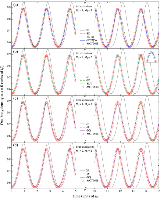
Figure 3. Time evolution of the one-body density at the center of the harmonic trap,  after an instantaneous quench of the interparticle interaction strength from
  to
to  (equations (50) and (51)). The result obtained using the mean-field GP theory (thin (black) line) strongly disagrees with the numerically exact result (open (red) circles) obtained using MCTDHB with 4 orbitals in all panels. Note that the results are plotted for
  on the left and
  on the right. (a) Results of the TD-RASSCF-B method using a single
  orbital,
  , and
, and 
 orbitals for different RAS schemes, namely -SD (dashed (green)), -SDTQ (dash-dot (purple)) and -SDTQ56 (thick (blue) line). For short time, the lines are on top of the MCTDHB result. (b) Results of the TD-RASSCF-B method using
  and
and  keeping the total number of orbitals constant for the -SD (dashed (green)) and -SDT (thick (blue) line) schemes. The results are on top of the MCTDHB curve, which show the good accuracy of the method. (c) Results using a single
  orbital,
  , and
, and 
 orbitals for only even excitations, i.e., -D (dashed (green)) and -DQ (dash-dot (purple)) RAS schemes. (d) Results of the TD-RASSCF-B method using
  and
and  keeping the total number of orbitals constant.
Download figure:
Standard image High-resolution imageIn the previous section, we showed that the RAS schemes with only even excitations provide accurate results for GS energy and reduce the numerical effort (see appendix  and
and  figures 3(c) and (d), respectively, and keep M = 4. For
  , figure 3(c), the results obtained with the -D and the -DQ schemes are in very good agreement with the MCTDHB results concerning both the frequency and the amplitude and start to deviate only for
  . In both cases, the number of configurations used to expand the wavefunction is substantially smaller than the expansion of the MCTDHB wavefunction with 7 and 22 configurations, respectively. When we use 2 orbitals in the
  -space both -D and -DQ provide the same results for the dynamics, see figure 3(d). For short time dynamics, the results are similar to the ones obtained previously with
  , but for a longer time, the oscillations remain in phase with the MCTDHB result, only the amplitude deviates for
  . The wavefunction of the -D scheme includes 38 configurations. Thus, the TD-RASSCF-B method provides an access to describe accurately the dynamics of the interacting system, while the mean-field GP theory fails even for short time. We obtain a good agreement in comparison to the MCTDHB method with a substantial reduction of the configurational space, using few tens instead of the few hundreds of configurations with the MCTDHB method. Moreover, the different parameters of TD-RASSCF-B method which define the wavefunction can be used to converge the results to the MCTDHB calculations. The implications of this reduction on the CPU time are discussed at the end of this section.
4.2. Breathing dynamics with

We continue the illustration of the TD-RASSCF-B method by considering a quenching from  to
to  (equation (51)). This interaction strength was used in [25] to benchmark the MCTDHB method. For the time interval considered here,
  , we find that the result obtained with the MCTDHB method using 8 orbitals and 19448 configurations is numerically exact, in agreement with [25]. As previously, the one-body density exhibits oscillations as a function of the time with a period
  , in perfect agreement with the analytical frequency
  . In comparison to the previous results in section 4.1, the shape of the oscillations indicates that the role of higher excited states is stronger as a large deviation from a simple cosine function,
  , is obtained. This is not surprising since the value of λ is now 5 times larger than the one of the previous example. Along with the MCTDHB result we report, for comparison, the result obtained using the mean-field GP theory, see figure 4(a), which strongly deviates from the MCTDHB result for
  with a larger amplitude in the oscillations and gives a lower frequency for the oscillations,
  . We start the TD-RASSCF-B simulations using M = 8 orbitals with one single
  orbital and
 orbitals, figure 4(a). For times between 0 and 2.5, the excitation schemes larger or equal to -SDTQ provide an accurate description of the dynamics, while the -SDTQ scheme includes 330 configurations in the wavefunction, i.e., a factor of ∼60 less than the MCTDHB. For longer times, the -SDTQ5678 RAS scheme with 6435 configurations is required to accurately describe the MCTDHB results, the lower excitation schemes give substantially different results. To improve the results of the TD-RASSCF-B method, we increase the number of orbital in
  and keep constant the total number of orbitals,
  . In figures 4(b)–(d) we report the results with
  , 3 and 4
  orbitals, respectively. In the case of
  , the -SDTQ56 RAS scheme, with 5412 configurations, provides a very accurate description of the dynamics for
  . For lower excitation schemes, the results are accurate for
  and using the -SDTQ scheme, the frequency of the oscillation at a longer time are correctly obtained, see figure 4(b). For
  , the results in figure 4(c) show that the -SDTQ5 RAS scheme including 6882 configurations converged to the MCTDHB results, while the -SDT scheme with 2276 configurations gives the correct frequency for the oscillation albeit with a smaller amplitude. Finally, figure 4(d) reports converged results for
  using the -SDT schemes, which includes 5216 configurations. Already, the -SD scheme with 2816 configurations is quite accurate for the considered time of propagation in comparison to the MCTDHB result.

Figure 4. Time evolution of the one-body density at the center of the harmonic trap,  after an instantaneous quench of the interparticle interaction strength from
  to
to  (equations (50) and (51)). The result obtained using the mean-field GP theory (thin (black) line) strongly disagrees with the numerically exact result (open (red) circles) obtained using MCTDHB with 8 orbitals in each panel. Note that the results are plotted for
  on the left and
  on the right. (a) Results of the TD-RASSCF-B method using a single
  orbital,
  , and
, and 
 orbitals for different RAS schemes, namely -SD (dashed (green)), -SDTQ (dash-dot (purple)), -SDTQ56 (thick (blue) line) and -SDTQ5678 (dash-dot (black)). (b) Results using
  and
and  keeping constant the total number of orbitals. For short time,
  , all RAS schemes are almost completely on top of the MCTDHB result. (c) TD-RASSCF-B simulations using
  and
and  orbitals, using the -SDT (solid (purple)) and -SDTQ5 (dash-dot (black)) RAS schemes. A very good agreement is obtained in comparison to the MCTDHB result. (d) Results of the TD-RASSCF-B method using
  and
and  orbitals using the -SD and -SDT schemes. This latter converges to the MCTDHB results but includes ∼4 times fewer configurations than the MCTDHB wavefunction.
Download figure:
Standard image High-resolution imageUsing different numbers of  orbitals and different RAS schemes points out that the number of configurations required to accurately describe the evolution of the system changes substantially. For instance, a similar accuracy is achieved for the -SDTQ5678 scheme with
  , the -SDTQ56 scheme with
  , the -SDT scheme with
  and the -SD scheme with
  . For each case, a smaller amplitude of the oscillations is observed in comparison to the MCTDHB for
  . But the numbers of configurations used in the wavefunction expansions are 6435, 5412, 2276 and 2816, respectively. Thus, for a comparable accuracy, the number of configurations can be divided by a factor ∼2 by choosing adequately the size of the
  -space and a factor ∼10 in comparison to the MCTDHB configurational space. The reduction of the configurational space impacts strongly the required CPU times of the simulations. For instance, the -SDTQ5678 RAS scheme with
  took ∼18.7 CPU hours, while the -SDTQ56 scheme with
  , the -SDT scheme with
  and the -SD scheme with
  took ∼19.8, ∼6.9 and ∼11.1 CPU hours, respectively, on a 2.4 GHz Intel E5-2680 CPU. Using these RAS schemes, the CPU time is drastically reduced in comparison to the ∼113.4 CPU hours on a 2.5 GHz Intel E5-2680 CPU needed to perform the MCTDHB simulation, but the dynamics is accurately described. Moreover, the -SDTQ5 RAS scheme with
  converged to the exact solution with ∼4 times less CPU time. Due to the drastic reduction in the size of configuration space, the CPU time needed to perform the TD-RASSCF-B calculations is substantially reduced.
We briefly summarize the findings concerning the dynamical evolution of trapped atoms after a quenching of the interaction strength of an attractive harmonic interaction. In the case of  , the MCTDHB theory converged to the numerically exact result for 4 orbitals. The TD-RASSCF-B method using different sizes of the
  -space and different RAS schemes can accurately describe the dynamics of the system characterized by
  with ∼4 times fewer configurations. Moreover, converged TD-RASSCF-B results were obtained with substantially less configurations, for instance with
  and the -SDT excitation scheme. In the case of
  , the exact solution was obtained with 8 orbitals using the MCTDHB method leading to 19448 configurations. A larger number of orbitals is needed for the stronger interaction between the particles. Accurate results were obtained with the TD-RASSCF-B method, reducing by a factor ∼10 the size of the configurational space and converged results were obtained with 4 times less configurations, for instance considering
  and the -SDT RAS scheme. Moreover, all calculations performed with the TD-RASSCF-B method were better than the mean-field GP theory, which failed to describe both scenarios. Physically, the sudden quench of the interaction between the particles projects the uncorrelated GS of the Hamiltonian of equation (50) onto the correlated many-body eigenstates of the Hamiltonian of equation (51). The time evolution of these latter eigenstates is trivial. They accumulate phase according to
  , with Ej the energy of the jth eigenstate, and the dynamics results from the coherent superposition of these eigenstates. Thus, the discrepancies that can be observed in figures 3 and 4 between the exact MCTDHB results and the different TD-RASSCF-B results asses the error of the different methods to correctly describe the relevant excited states for the dynamics. Moreover, the fact that the RAS schemes with only even excitations (figure 3(c)) provide an accurate description of the dynamics highlights the role of the correlation as the configurations are only coupled through the two-body operator, see equations (8) and (10).
5. Conclusion and outlook
In this work, we presented a general theory for the TD-RASSCF method for indistinguishable particles, which includes the derivation obtained previously for fermions (TD-RASSCF-F) [91, 92, 94] and extended it for systems of spinless bosons (TD-RASSCF-B). This TD-RASSCF-B method includes, as limiting cases, the (TD)-GP and the MCTDHB theories and provides a way to tackle the exponential growth of the configurational space in the MCTDHB method. The EOM were derived for two families of RAS schemes, which give the possibility to restrict the full-configurational description of the MCTDHB wavefunction. Through a set of numerical examples, we have shown that the method can provide an accurate description of the static properties of the ground-state of the system. In the case of hundreds of particles, the method can lead to results beyond the reach of the MCTDHB method. The TD-RASSCF-B provides a better accuracy by including more orbitals while constraining the number of configurations and reducing considerably, in that way, the size of the configurational space. In the ground-state calculations, the flexibility of the RAS scheme allowed us in this sense to identify clearly the physics that needs to be accurately represented: (i) Even (two-body) excitations are more important than single excitations. (ii) While most particles remain in the motional ground-state (SCF) orbital, it is important to account for the relatively fast motion of a few particles by including many orbitals. In this sense, the TD-RASSCF-B method paves the way for numerical investigation of intermediate system sizes with a few tens to hundreds of bosons with a better accuracy than what is possible with the MCTDHB method. We also provided a comparison between the TD-GP, the MCTDHB and the TD-RASSCF-B methods in the case of breathing dynamics induced by a sudden quenching of the interaction strength with two different initial conditions. As the MCTDHB method, the TD-RASSCF-B method does not have any restriction on the choice of the two-body interaction potential used. This was illustrated by the use of a non-contact harmonic interaction between the bosons. We showed that for the studied interaction quench, often used in cold atom experiments, the TD-GP approach becomes inaccurate within a fraction of an oscillation period of the harmonic trapping potential. Using as a reference the numerically exact result obtained from the MCTDHB method, we showed that the TD-RASSCF-B method is always more accurate than the mean-field TD-GP theory to describe the dynamics of the system. Moreover, using different RAS schemes and partitions of the  -space we obtained very accurate results with substantially less configurations and thus less CPU time than with the MCTDHB method. Finally, as was the case for the ground-state calculations, the RAS scheme allowed us to identify the nature of the excitations that are important for this kind of dynamics. In this case accurate results can be obtained using only even SCF excitations, highlighting the importance of the two-body interaction. In the future the accuracy and numerical efficiency of the TD-RASSCF-B method can be exploited further to solve the TDSE beyond the mean-field approach, and for situations out of reach by other time-dependent wave function based methods. Dynamical effects such as the four wave mixing process [110] used to produce correlated atom beams [111] or the dynamics of bright [112, 113] and dark [114, 115] solitons can be investigated ab initio beyond the mean-field TD-GP theory. In addition, the dynamics induced by a time-dependent Hamiltonian can also be explored using the TD-RASSCF-B method, such as in the case of periodically driven optical lattices [116, 117]. In all of this, the RAS concept will be highly operational in identifying the most important excitations, and hence the physical nature of a given process, as was the case in the illustrative applications of the present work.
Acknowledgments
The authors are indebted to Dr Haruhide Miyagi for useful discussions. This work was supported by the ERC-StG (Project No. 277767-TDMET), and the VKR center of excellence, QUSCOPE.
Appendices
In these appendices we provide a brief description of the implementation the TD-RASSCF-B method. The implementation is rather similar for bosons and fermions in the sense that the set of equations that we have to solve, i.e. Equations (15), (25) and (38) or (43), only depend on the type of particles through the creation and annihilation operators and the set of configurations  . Moreover, additional illustrative examples are presented and discussed.
Appendix A.: Compact representation of the wavefunction
Our implementation is based on the general mapping of bosonic operators in Fock space introduced in [118] and implemented, for instance, for bosons [119] and fermions [27] in the framework of multi-configurational TD methods. Assuming M orbitals and N bosons, the configurations are expressed using the occupation number formalism, where  , represents a configuration with n1 bosons in the orbital
  , n2 bosons in the orbital
  , etc. Such a configuration is indexed by an unique integer J defined as,
Thus, for each configuration we store its complex coefficient CJ in an array according to the index J provided by the above mapping. In [119], this mapping was employed to avoid the storage of the configuration vectors  , which can be prohibitively memory consuming in the case of the MCTDHB method. Thus, to access the coefficient of the configurations, a set of M-nested loops over the occupation number ni is used to span the full configurational space and to compute, using equation (A1), the respective indexes. In the case of the TD-RASSCF-B method only a selected number of configurations are used to expand the wavefunction, and the scheme of [119] is not readily applicable in the sense that we want to avoid explicit use of the full configurational space. Instead we follow a different strategy for indexing the RAS configurations. We introduce M1 and M2 the number of orbitals in the
  and
and  spaces, respectively. For
  , i.e., configurations with particles only in
  , see equation (39), we enumerate all possible configurations, evaluate their index, using equation (A1), and store them. Then for the excited configurations, i.e., configurations with one or more particles in
  , we introduce the excitation number nexc which is equivalent to the number of particles in
  . The number of remaining particles in
  is
is  . For each excitation we enumerate the configurations of
  particles in the
  orbitals and compute their index. The same is performed for the configurations with nexc in
  orbitals. Then the permanents for the total number of bosons are obtained by combining them,

where  is an array of dimension
  , with
  (
( ) the total number of configurations obtained from arranging the
  (nexc) particles in the
  (
( ) orbitals. We evaluate the indexes of the configurations resulting from the
  subsystem,
  , and from the
  subsystem,
  , applying equation (A1) for the subsystems, separately. The index of the configuration with the total number of bosons is build as a three components array defined by
  , which stores the position of the configuration in the configurational vector. This scheme is thus applied for all excitations, nexc, included in the RAS scheme. With this storage or construction of the wavefunction, for a given configuration we have access to its coefficient in the following way. (i) We evaluate the index
  for the
  subsystem, (ii) we evaluate the index
  for the
  subsystem, (iii) we know or evaluate the excitation, nexc, of the configuration (iv) we access to the index of the coefficient which is stored and the three component array at position
  . This scheme has, as a draw back, the requirement to store the list of occupation numbers and the indexes to be efficient for numerical evaluation. But the idea behind the TD-RASSCF-B method is to reduce the size of the configurational space, which made such a storage manageable for the applications done so far.
Appendix B.: Applying operators in second quantization
In second quantization, the action of the Hamiltonian of equation (8) on the wavefunction requires the application of annihilation and creation operators and multiplication by the matrix elements of the one- and two-body operators. To know the action of the Hamiltonian, we first need to know the action of the creation-annihilation operators [118, 119]. Concerning the one-body term, we have,

For a full-configurational wavefunction, the resulting configuration belongs to the configurational space and its index can be determined as described in appendix A. Now, considering the action on the wavefunction,

with  the new configuration resulting from the action of
  on the initial configuration
  . The result can be interpreted as a reordering of the configuration in the wavefunction, as in equation (B2) or inversely to a reordering of the coefficients with a new factor (
 ) if the configuration are reorganized in the initial order, i.e.,

In the basis of the configurational states,  , the wavefunction is characterized by its coefficients only, and is stored as a vector. The new set of coefficients,
  , resulting from the action of
  , is obtained as,

In practice, we apply  on the bra
  , which provides a new configurational state
  . The configurational vectors are orthonormal, and only the configuration
  in the sum remains from the projection. Thus, we evaluate the index of
  to directly access the coefficient CJ, i.e.,

The action on the total wavefunction is obtained by repeating these operations for each configuration, providing a new coefficient vector. In the case of the RAS wavefunction, the configuration obtained from the successive application of the annihilation and creation operators may not belong to the configurational space. Nonetheless, the scheme explained above can be applied. In addition, a test to check if the resulting configuration remains in the RAS space has to be performed. This naive approach can be easily improved thanks to the representation of the wavefunction used and its indexing (see appendix A). The orbitals  , on which the operators
  act, can (i) belong to
  only
only  , (ii) belong to
  only
only  , or belong to
  and
and  , (iii)
  and (iv)
  . For (i) and (ii) the excitation, or the number of particles in
  , do not change in the resulting configuration. For the situation (iii) one particle is removed from
  and added in
  and the opposite happens for (iv). The excitation of the final configuration is thus known without counting the number of particles in
  , which is required to determine the index of the configuration. Moreover, to always remain in the RAS configurational space, the case (iv) is never applied to the configuration with the maximal number of excited particles allowed for the general RAS scheme (section 2.2.2.4), and both (iii) and (iv) are not occuring for the scheme with only even excitations (section 2.2.2.3). The action of the one-body operator of the Hamiltonian is now straightforward, the coefficient vectors obtained by applying the
  operators are multiplied by the corresponding matrix element hji (equation (9)) and summed for each couple of
  , with the restriction mentioned above for the RAS wavefunction. The two-body operator, see equation (10), included in the Hamiltonian of equation (8) and the four- and six-order tensors specific to the RAS schemes (equations (44) and (45)) can be evaluated using the same strategy as the one detailed for the one-body operator. We mention that using the commutation relation for bosonic creation and annihilation operators can substantially reduced the numerical cost. For instance, if we consider the chain of operators
  , we have the equalities
  .
.
Appendix C.: Numerical implementation for the TD-RAS equations
The EOM for the TD-RASSCF-B and F methods, equations (15), (25) and (38) or (43), are solved to obtain the time derivative of the coefficients and orbitals. The main difference with the MCTDHB and F methods results from the evaluation of the matrix elements  . These elements are evaluated from equations (38) or (43) depending on the RAS scheme used, but both are solved in the same way. We recall that the matrix
  , with elements
  , is anti-hermitian and thus
  , here
  and
and  correspond to orbitals of the
  and
and  subspace, respectively. Writing down equations (38) or (43) for any set of orbitals
  , provides a system of
  linear equations with
  unknowns. Introducing a composite index for the couple of
  , this system can be written in a matrix form,

where the matrix  , of dimension (
 ,
,  ), contains the values of
  or
or  , for all set of
  and
and  . The vector
  , of dimension (
 ), contains the rhs of equation (38) or (43) for each set of
  and the vector
  with the same dimension as
  contains the unknown values of
  and the matrix elements of the one-body operator. The system of linear equations, equation (C1), can be solved using standard numerical routines included, for instance, in the LAPACK library [120]. The values for
  are trivially obtained from the elements
  of the vector
  ,
,

After evaluating the matrix elements  , the time derivative of the coefficients
  can be computed from equation (16) and the contribution of the
  -space orbitals to the time derivative of the orbitals is obtained from,

It remains to evaluate the contribution from the orbitals of the  -space, i.e.
  from equation (25). This latter can be expressed in a matrix form,

with  the one-body reduced density matrix,
  a vector collecting the time derivative of the orbitals,
  and
and  are both vectors with elements
  and
and  , respectively. To obtain equation (C4), we used the fact that
  commutes with the projector
  , as easily seen from the equality
  . Multiplying on the left by the inverse of the one-body density matrix,
  , we have, for the orbital
  ,
,

The right hand side of the above equation is similar to the one that is solved in the MCTDH-based methods [67, 68, 70] and to avoid singularities in the inverse of the one-body reduced density matrix and in equation (C1) for the matrix  , we follow the numerical implementation used for the MCTDH method [121] . The method uses a regularized one-body density matrix defined as [121],

with  a small real number (see appendix E.1). The same regularization is used for the matrix
  . The numerical implementation of the projector onto the
  -space orbitals also follows [121] to ensure stability of the orthonormality of the orbital during the propagation. The projector
  is numerically expressed by,

where  is the overlap matrix of the time-dependent orbitals. Thus, the projector defined in equation (C7) remains orthonormal even if the orthonormality of the orbitals is lost as long as they remain linearly independent.
Appendix D.: Numerical efficiency of the method
Comparing the efficiency between different methods is a difficult task as it depends on the specific implementation and integration schemes used. Nonetheless, we can roughly estimate the number of operations required to evaluate the time derivative of the orbitals and coefficients and compare the MCTDHB and TD-RASSCF-B methods in this way. We denote by Ngrid the number of grid points that are used to describe the time-dependent orbital in the time-independent basis, usually a DVR [122], which is the same for both methods. Starting with the MCTDHB method, at each evaluation of the time derivative the matrix elements of the two-body operator vklij (equation (10)) and the two-body reduced density matrix  (see text above equation (25)) are computed. These updates require
  and
and  operations, respectively, with
  the configurational space of the MCTDHB wavefunction evaluated from equation (3). Then computing the time derivative of the coefficients and the orbitals require on the order of
  and
and  operations, respectively. The total cost is thus, approximately,
  . Considering now the case of the TD-RASSCF-B method. The evaluation of the matrix elements of the two-body operator and the calculation of the
  -space equations for the time derivative of the orbitals require the same number of operations as with the MCTDHB method, i.e., on the order of
  operations, respectively. The evaluation of the time derivative of the coefficients and the matrix elements of the two-body reduced density matrix scale as
  , with
  the configurational space for the considered RAS scheme. In addition, we also need to solve the
  -space equations, which requires on the order of M4 operations for excitation schemes with only even excitations (see equation (38)) and
  for the general RAS scheme (see equation (43)), with
  the number of configurations including
  particles in the
  -space. The total number of configurations included in the RAS wavefunction for the general excitation scheme is evaluated using equation (5) and
  is the last term of the summation. The dimension of the configurational space,
  , including only even excitations can be evaluated in a similar way,

Combining the results for the general RAS scheme, the number of operations required to evaluate the time derivative of the coefficients and orbitals scales as  and in the case of only even excitations it scales as
  . To compare the numerical cost between the MCTDHB and TD-RASSCF-B methods, we can introduce
  , the difference between the MCTDHB and TD-RASSCF-B operations to remove the constant number of operation resulting from Ngrid,

From the expression of  , a positive value represents a computational gain with the TD-RASSCF-B in comparison to the MCTDHB method, while a negative value is obtained when the MCTDHB method is more efficient. In the case of a scheme with only even excitations,
  is proportional to the size difference of the MCTDHB and TD-RASSCF-B configurational spaces and is always positive, which means that the TD-RASSCF-B method is always more efficient. In the case of the general excitation scheme the sixth-order tensor of the
  -space equations, equation (45), can provide an overhead for the computation. To illustrate the computational efficiency we evaluate
  for 10, 50 and 100 bosons in M = 2 to 8 orbitals, see figure D1. For the TD-RASSCF-B, we consider the case of a single
  orbital and
  orbitals in
  . From the figure, the case with only even excitations reduces the computational cost almost exponentially for increasing number of orbitals for any number of particles, which results from the efficiency of solving the
  -space equation. In the case of the general RAS scheme, there is always a value of
  which leads to more operations in the TD-RASSCF-B than in the MCTDHB method, due to the evaluation of the six-order tensor in the
  -space equation. But as shown in figure D1, this value is rather large, i.e.
  for 10,
  for 50 particles and
  for 100 particles for the schemes depicted in figures D1(a), (b) and (c), respectively.

Figure D1. Difference between the number of operations used to evaluate the time derivative of the wavefunction with the MCTDHB and TD-RASSCF-B method. The difference  is defined by equation (D2) in appendix D. We report the value of
  as a function of the number of orbitals for a system consisting of (a) N = 10 particles, (b) N = 50 particles and (c) N = 100 particles. The circles indicate the results for general RAS schemes (left axis) and the diamond symbols depict the results for the case of RAS schemes with only even excitations ((red) right axis). For the RAS schemes with only even excitations, the number of operations is always fewer than for the MCTDHB method. For the general RAS schemes, for high excitation schemes and large numbers of orbitals the number of operations can be larger than the one of the MCTDHB method. For instance, considering N = 10 particles (panel (a)) and the -SDTQ56 scheme (blue circle) the number of operations with the TD-RASSCF-B method is higher than with the MCTDHB method for
  orbitals. The same happens for N = 50 particles and the −40 scheme with
  orbitals and for N = 100 particles and the scheme −90 with
  orbitals.
Download figure:
Standard image High-resolution image
Appendix E.: Numerical parameters and more illustrative examples
E.1. Numerical parameters
To solve numerically the EOM of the MCTDHB and TD-RASSCF-B theories, the time-dependent orbitals are expanded on a time-independent basis or primitive basis, which consists of a sine discrete variable representation (DVR), see [69]. We use 101 basis functions in a box ![$[-8,8]$](https://content.cld.iop.org/journals/1367-2630/19/4/043007/revision1/njpaa6319ieqn611.gif) and compare the results with larger basis sets to ensure the convergence of the energies presented in table 1 (see section 3) and II (see appendix E.2). We numerically integrate the EOM using different integration algorithms, namely the 4th order runge-kutta (RK) [123], the adaptive time-step 5th order RK and the Adams-Bashforth-Moulton (ABM) predictor-corrector as also implemented in the Heidelberg MCTDH package [124]. Each simulation always used the same integration routine for both coefficients and orbitals. The different integration schemes were tested against each other and we report the results obtained using the ABM integrator to the 7th order, as it is the most efficient. The error tolerance for the integration has been fixed to 10−8, and we controlled the convergence of our results with respect to this parameter by performing simulations with higher and lower error tolerances. During a calculation, the inverse of the reduced one-body density matrix can be singular when one or more of the natural orbitals are unoccupied. To prevent the singularity we used a regularization scheme, see appendix C, with a regularization parameter
and compare the results with larger basis sets to ensure the convergence of the energies presented in table 1 (see section 3) and II (see appendix E.2). We numerically integrate the EOM using different integration algorithms, namely the 4th order runge-kutta (RK) [123], the adaptive time-step 5th order RK and the Adams-Bashforth-Moulton (ABM) predictor-corrector as also implemented in the Heidelberg MCTDH package [124]. Each simulation always used the same integration routine for both coefficients and orbitals. The different integration schemes were tested against each other and we report the results obtained using the ABM integrator to the 7th order, as it is the most efficient. The error tolerance for the integration has been fixed to 10−8, and we controlled the convergence of our results with respect to this parameter by performing simulations with higher and lower error tolerances. During a calculation, the inverse of the reduced one-body density matrix can be singular when one or more of the natural orbitals are unoccupied. To prevent the singularity we used a regularization scheme, see appendix C, with a regularization parameter  . Again, the convergence with respect to the value of was ensured by performing calculations with
  and no significant difference in the results was found. For instance, the reduced one-body density matrix is singular when computing the ground state of the Hamiltonian of equation (50), but the energy is known analytically (
 ) as the particles do not interact with each other. The GS energies obtained numerically with
  are all accurate up to 10−13 for any number of orbitals and excitations. We calculate the GS energy using imaginary time propagation [125] of the EOM and give all energies in units of E0.
E.2. More illustrative examples
In this Appendix, we consider the same system as the one presented in section 3 except that the interaction strength is now 10 times larger with  , see equation (46). We perform an analysis of the GS energy obtained with the different methods, similarly to section 3, and the results are reported in table 2. The reference for the correlation energy (see equation (48)) is
  , see table 2. This value is much larger than the one obtained in section 3 with
  and can be explained by the stronger interaction between the particles. Indeed, for a stronger interaction strength, the energy of the system is lowered by allowing the particles to occupy higher orbitals, i.e., orbitals leading to higher kinetic and potential energies, such that the interaction energy is reduced. In the mean-field GP theory, this is not possible as only one orbital is used to describe the wavefunction. The orbitals that diagonalize the reduced density matrix and their respective eigenvalues, i.e., their natural occupations, can be used to characterize the system. If the largest eigenvalue is of the same order as N, the system is condensed [109]. As the GP wavefunction includes a single orbital, it can only describe condensed systems. If more than one eigenvalue is of the order of N, then the system is fragmented (see [126] and the discussion in [83]). We find that, indeed, the natural occupation of the lowest natural orbital in the MCTDHB calculation using 5 orbitals decreases from an occupation of
  for
for  to an occupation of
  for
for  . This slightly larger depletion of the condensate has a strong impact on the correlation energy, and the mean-field GP theory provides a less accurate description of the system. We point out that increasing the number of orbitals from 4 to 5 in the MCTDHB calculations gives an energy difference
  , see table 2, which means that the energy does not converge below this value. The relative correlation energy, see equation (49),
  ,
,  and
and  include
  ,
,  and
and  of
of  , respectively.
Table 2.
Same as table 1 but for ground-state energies of 100 bosons trapped in a 1D harmonic potential interacting through a contact potential with a strength  .
.
| Orbitals | ||||||||
|---|---|---|---|---|---|---|---|---|
| Method | 1 | 2 | 3 | 4 | 5 | 6 | 7 | 8 |
| All excitations | ||||||||
| MCTDHB | 193.5509587 | 193.0154216 | 192.6308389 | 192.3920265 | 192.2138048 | — | — | — |
| (1) | (101) | (5151) | (176851) | (4598126) | (96560646) | (1705904746) | (26075972546) | |
| -SDT | — | 193.0783470 | 192.7594351 | 192.5665491 | 192.4187690 | 192.3153377 | 192.2315684 | 192.1681159 |
| (4) | (10) | (20) | (35) | (56) | (84) | (120) | ||
| -SDTQ5 | — | 193.0310688 | 192.6591396 | 192.4322339 | 192.2605383 | 192.1396169 | 192.0434375 | 191.9701535 |
| (6) | (21) | (56) | (126) | (252) | (462) | (792) | ||
| -SDTQ567 | — | 193.0191782 | 192.6370892 | 192.4017271 | 192.2250102 | 192.1000115 | 192.0013608 | 191.9259461 |
| (8) | (36) | (120) | (330) | (792) | (1716) | (3432) | ||
| -SDTQ56789 | — | 193.0162747 | 192.6321926 | 192.3943825 | 192.2165110 | 192.0903987 | 191.9911974 | 191.9152346 |
| (10) | (55) | (220) | (715) | (2002) | (5005) | (11440) | ||
| -10 | — | 193.0158613 | 192.6315747 | 192.3933448 | 192.2153160 | 192.0890211 | 191.9894655 | 191.9133983 |
| (11) | (66) | (286) | (1001) | (3003) | (8008) | (19448) | ||
| -15 | — | 193.0154291 | 192.6308506 | 192.3920555 | 192.2138378 | 192.0872814 | 191.9879161 | 191.9117429 |
| (16) | (136) | (816) | (3876) | (15504) | (54264) | (170544) | ||
| -20 | — | 193.0154220 | 192.6308392 | 192.3920271 | 192.2138055 | 192.0872403 | 191.9878729 | — |
| (21) | (231) | (1771) | (10626) | (53130) | (230230) | (888030) | ||
| -23 | — | 193.0154216 | 192.6308389 | 192.3920265 | 192.2138049 | 192.0872393 | 191.9878720 | — |
| (24) | (300) | (2600) | (17550) | (98280) | (475020) | (2035800) | ||
| -25 | — | 193.0154216 | 192.6308389 | 192.3920265 | 192.2138048 | 192.0872393 | 191.9878719 | — |
| (26) | (351) | (3276) | (23751) | (142506) | (736281) | (3365856) | ||
| Even excitations | ||||||||
| -D | — | 193.1320396 | 192.8258797 | 192.6453389 | 192.5031705 | 192.4050140 | 192.3243169 | 192.2636708 |
| (2) | (4) | (7) | (11) | (16) | (22) | (29) | ||
| -DQ | — | 193.0449780 | 192.6788633 | 192.4619220 | 192.2951569 | 192.1793448 | 192.0861393 | 192.0157234 |
| (3) | (9) | (22) | (46) | (86) | (148) | (239) | ||
| -DQ6 | — | 193.0227865 | 192.6439550 | 192.4175380 | 192.2457797 | 192.1259116 | 192.0303689 | 191.9579281 |
| (4) | (16) | (50) | (130) | (296) | (610) | (1163) | ||
| -DQ68 | — | 193.0171558 | 192.6356968 | 192.4065816 | 192.2338183 | 192.1129247 | 192.0169500 | 191.9440484 |
| (5) | (25) | (95) | (295) | (791) | (1897) | (4166) | ||
| -10 | — | 193.0158072 | 192.6338334 | 192.4039516 | 192.2310023 | 192.1098389 | 192.0137924 | 191.9407800 |
| (6) | (36) | (161) | (581) | (1792) | (4900) | (12174) | ||
| -20 | — | 193.0154216 | 192.6333324 | 192.4031759 | 192.2301918 | 192.1089342 | 192.0128774 | 191.9398292 |
| (11) | (121) | (946) | (5786) | (29458) | (129844) | (508937) | ||
| -30 | — | 193.0154216 | 192.6333323 | 192.4031756 | 192.2301915 | 192.1089338 | 192.0128771 | — |
| (16) | (256) | (2856) | (24616) | (174624) | (1061208) | (5678340) | ||
Starting the discussion with the general RAS schemes, see table 2, we note that to converge to the MCTDHB energies and thus include 100% of the relative correlation energies,  with X = 2 to 5, large values of
  are required. For the -SDTQ5 RAS scheme we find that the correlation energy includes
  of
of  , the -10 RAS scheme includes
  of
of  , the -15 RAS scheme includes
  of
of  and the -20 RAS scheme is converged with more than
  of
of  . These results are obtained irrespectively of the number of orbitals, i.e., X = 2 to 5. Even if large values of
  are used, the expansion of the wavefunction using the -20 RAS scheme includes
  configurations for 5 orbitals while the MCTDHB wavefunction includes
  configurations. We also use RAS schemes with only even excitations and we report the results in table 2. Similarly to the case with
  , see section 3, we find that, except for 2 orbitals, the energy does not converge to the MCTDHB energy, irrespective of the value of
  used. Thus the energies obtained with 3, 4 and 5 orbitals include
  ,
,  and
and  of the respective
  with the -20 RAS scheme, which is converged. For similar numbers of configurations the general RAS scheme provides more accurate results but remains more demanding in term of computation, see appendix D. It is important to keep in mind that the convergence with respect to the number of orbitals is
  and a convergence to
  is achieved with the -SDTQ5 excitation scheme and the -DQ excitation scheme (table 2). As previously, the configurational space of the MCTDHB wavefunction becomes unworkable for more than 5 orbitals, but the TD-RASSCF-B method can include more orbitals. At the level of the -SDT scheme and 8 orbitals and for higher excitation schemes with 6 to 8 orbitals, the GS energy is always below the energy obtained with the MCTDHB method with 5 orbitals, see table 2. In the same way, using only even excitations provides more accurate results for excitation schemes higher than -D. As a remark, we obtain an energy ∼0.3 below the energy of the MCTDHB method with 5 orbitals by using the -15 RAS scheme with 8 orbitals, see table 2.