


Abstract
Many quantum dot qubits operate in regimes where the energy splittings between qubit states are large and phonons can be the dominant source of decoherence. The recently proposed charge quadrupole qubit, based on one electron in a triple quantum dot, employs a highly symmetric charge distribution to suppress the influence of long-wavelength charge noise. To study the effects of phonons on the charge quadrupole qubit, we consider Larmor and Ramsey pulse sequences to identify favorable operating parameters. We show that phonon-induced decoherence increases with the qubit frequency, in contrast to the effects of charge noise. We also show that there is an optimum value of the tunnel coupling of the qubit at which the decohering effects of phonons and charge noise are small enough to be consistent with single qubit gate fidelities > 99.99%.
Export citation and abstract BibTeX RIS
1. Introduction
The past two decades have witnessed remarkable advances in the development of qubits in semiconductor-based systems [1–17]. Qubits constructed using electrons confined in lateral quantum dots (QDs) have been realized experimentally in different forms, including single-spin qubits [4–6, 8, 18, 19], singlet-triplet qubits [20, 21], QD hybrid qubits [22–24], exchange-only qubits [25–27], and charge qubits with different numbers of electrons [23, 28–30]. One of the main sources of qubit decoherence in each of these systems is charge noise, which can arise from high-temperature electrical noise in the voltage controls or the motion of defects and free charges in the heterostructure. The recently proposed charge quadrupole qubit, formed of one electron in a triple QD, is robust against uniform electric field fluctuations due to the high symmetry of its basis states [31, 32]. The qubit states are symmetric with respect to the central QD, thus forming a decoherence-free subspace, which is well-known for spin qubits [33–35], but novel for charge qubits. However, as for all qubits relying on a symmetric operating point, phonons can break this symmetry and cause decoherence. Indeed, phonons have been shown to be a significant source of decoherence for many types of QD qubits [13, 36–46].
Here we study theoretically the decoherence of a charge quadrupole qubit arising from its coupling to phonons. In addition to decoherence between qubit states, we account for the effects of a leakage state. The leakage state is not coupled to the qubit subspace in the ideal case, but phonons break the symmetry of the qubit and consequently induce a coupling. The effects of phonons are greatest when the energy separation between the states is large, because the phonon density of states increases with energy and the electron–phonon matrix elements depend on momentum. To characterize the effects of phonon-induced decoherence and to identify favorable operating parameters for the qubit, we study Larmor and Ramsey pulse sequences, which can be used to implement arbitrary single-qubit gate operations. An important parameter for qubit control is the tunnel coupling, which strongly affects the qubit energy. Since phonon-induced decoherence increases as the tunnel coupling increases, and the decoherence arising from charge noise [31, 32] decreases as the tunnel coupling increases, both sources of decoherence must be considered to identify the optimal working regime for the qubit. We demonstrate that there is a working regime where qubit infidelity from both these processes is less than 0.01%.
The paper is organized as follows. In section 2 we present the Hamiltonian of a charge quadrupole qubit interacting with a phonon bath. In section 3 we consider the time evolution of the density matrix describing the qubit subspace and a leakage state. We discuss phonon-induced decoherence rates in section 4. Then we compare phonon-induced infidelity to the infidelity due to charge noise in section 5. A discussion of how to reduce other possible sources of decoherence in such devices is presented in section 6. Details of the calculations and additional information are provided in the appendices.
2. Model
2.1. Electron in a triple QD
The charge quadrupole qubit is formed in a triple QD that hosts one electron [31], as illustrated in figures 1(a) and 1(b). The qubit is operated in a symmetric fashion, such that the energies of the first and third QDs are the same and the middle QD has the same tunnel coupling to the two outer QDs. However, phonons can perturb the potential of the triple QD, as shown in figure 1(c), giving rise to decoherence.
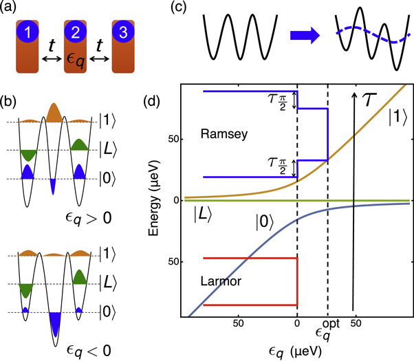
Figure 1. (a) The charge quadrupole qubit, introduced in [31], consists of three quantum dots (blue circles), which are controlled by metallic top gates (red rectangles), and coupled via tunnel barriers. The quadrupolar detuning  is controlled by the central gate. (b) A cartoon sketch of the wave functions of the basis states
  (blue),
  (green), and
  (orange), for positive (top) and negative (bottom)
  q. (c) Qualitative illustration of the effect of a transverse phonon on the triple dot potential, resulting in decoherence. (d) The spectrum of a charge quadrupole qubit. Insets show the pulse sequences used to implement Larmor and Ramsey qubit operations studied here (vertical axis is time).
Download figure:
Standard image High-resolution imageTo model this system, we consider electron wave functions in the x–y plane of a quantum well, which are constructed from the ground states of harmonic oscillator potentials that approximate the QD confinement [47]. For the left, right, and central QDs these are given by


respectively. Here, a is the interdot distance and l characterizes the radius of the dots. Both a and l are assumed to be the same for all three QDs. As the dots are situated rather close to one another, there are overlaps between these states,  . To construct orthonormal wave functions of an electron in a triple QD we must take these overlaps into account. Note that we include the overlaps
  and
and  but not
  , because the separation between the left and right dots is much larger than between an outer dot and the central dot. Generalizing a well known procedure for double dots [47, 48] to the three-dot problem, we construct the orthonormal wave functions for an electron to be in the left, right or central QDs of the triple QD (see appendix B for details)


where  , and φ(z) represents the component of the wave function in the heterostructure growth direction, as described in detail in appendix A. We have checked that the results do not depend on the detailed form of φ(z). This insensitivity comes from the fact that the phonons responsible for transitions have wavelengths that are much greater than the thickness of φ(z). In this work, we therefore take φ(z) to have a simple Gaussian envelope with a full width at half maximum of 4.7 nm.
As described in [31], the Hamiltonian of an electron in a triple QD in the  basis is

where tA, tB are tunnel couplings between the dots, and UL, UC, and UR are the potentials of the left, central, and right QDs, which are defined by the gate voltages. The dipolar and quadrupolar detuning parameters are defined as  and
and  , respectively. When
  and d = 0, H0 describes a charge quadrupole qubit [31]. Gate operations can be performed by varying the quadrupolar detuning q in time, as illustrated in figure 1(d).
In addition to the dipolar and quadrupolar detunings, several other experimental parameters can be tuned, including the dot separation a, the wave function extent that characterizes the radius of the dots, l, the tunnel coupling t, and the temperature T. To estimate the value of t, we model t as the tunnel coupling between the two sides of a double well potential  , where
  is the transverse effective mass of an electron in Si. With details given in appendix C, we obtain

Note that for this double well potential form, the detuning between the wells is zero, and we have ignored any dependence of t on the detunings. However it allows us to estimate how strongly the change in a or l affects tunnel coupling. From equation (6), we see that  grows rapidly with l. Changing the tunnel coupling is found to have a strong effect on decoherence rates, as we will show below.
The eigenstates of the Hamiltonian H0 when d = 0 form a convenient basis for the quadrupole qubit, given by


Here,  and
and  represent the qubit subspace and
  is the qubit energy splitting. The state
  represents a leakage state that decouples from the qubit subspace in the absence of environmental noise. The wave functions are illustrated schematically in figure 1(b). In the following, we use the
  basis to study the time evolution of the qubit coupled to phonons.
2.2. Interaction with the phonon bath
In this subsection we show how we include phonons in our model. The Hamiltonian of an electron in a triple QD coupled to the bath of phonons is given by  , where Hph is the phonon bath Hamiltonian defined as
  with
with  and
and  are annihilation and creation operators for phonons of mode
  (corresponding to one longitudinal and two transverse acoustic modes) and wave vector
  , with the phonon frequency
  . The electron–phonon interaction is described by
  .
.
In this work, we will study triple QDs constructed in Si-based heterostructures, which can be, for example, Si/SiO2 or Si/SiGe. The electron–phonon interaction Hamiltonian in bulk Si is given by [49–51]

where  is a strain tensor defined as [45, 51]


where Ξd and Ξu are deformation potential constants,  is a displacement operator,
  denotes the position of the electron,
  , vs is the speed of sound for each of these modes, ρSi is the mass density of bulk Si, and V is the volume we consider. The polarization vectors are chosen as follows:
  ,
,  , and
, and  , so that in equation (12) one has ∓l = −,
  , and
, and  . Explicit expressions for the polarization vectors are given in appendix D. We assume the following parameters for Si: deformation potential constants 5 and 8.77 eV [50], speed of sound for longitudinal phonons
  m s−1 and transverse phonons
  m s−1 [52, 53], the bulk mass density 2.33 g cm−3.
Evaluating H in the regime used for the charge quadrupole qubit in the  basis yields
where PLL, PCC, PRR, PLC, PCR are electron–phonon interaction matrix elements, defined as  . Note that we have neglected the matrix elements PLR here because the corresponding wave functions have a negligible overlap.
In the following, we treat  as a perturbation and study how the electron–phonon interaction affects the dynamics of the three-level system
  .
.
3. Time evolution of the three-level system
To investigate the time evolution and decoherence of the qubit, we employ the Bloch–Redfield formalism [39, 54, 55]. First, we apply to the full Hamiltonian H the transformation Ud that diagonalizes H0, yielding  . Similarly, we define
  . We then derive the equation for the time evolution of the density matrix of our three-level system in the
  basis following the procedure described in [54] (for the full derivation see appendix E): (1) write down the von Neumann equation, (2) trace over phonon degrees of freedom, (3) apply the Born–Markov approximation. The Markov approximation is justified here by the fact that the phonons transit the triple QD in a period
  [39], which is by several orders of magnitude shorter than the decoherence times we present below. The gate times we consider in section 5 are ∼2–11 times larger than τcorr. The resulting equations for the elements of the density matrix ρ are

where the indices n, m, j, k refer to the eigenstates of H0,  , and the frequency ωnm is the splitting between states n and m. The decoherence rates due to the electron–phonon interaction,
  and
and  , are
, are


where τ is time. Here, the angular brackets denote an average over phonon degrees of freedom,  , where ρph is the thermal equilibrium state of the phonon bath. The notation
  indicates that
  is expressed in the interaction representation, defined as
  . From equations (15) and (16) we see that Bloch–Redfield formalism takes into account all transitions between the states.
In the following, we use equation (14) to calculate qubit evolution during Larmor and Ramsey pulse sequences, implemented for qubit manipulations [1, 56] and shown in figure 1(d). The Larmor pulse sequence is performed in the following way: the quadrupolar detuning is suddenly pulsed from a large negative value to q = 0, where the qubit freely precesses for time τ, and then suddenly pulsed back to its initial value. It is used to perform rotations about the  axis of the Bloch sphere. For the Ramsey pulse sequence, we first pulse from large negative detuning to q = 0, allowing it to evolve long enough,
  , to perform an X(π/2) rotation, then the system is pulsed to a required positive detuning, where it evolves freely for time τ, and then is pulsed back to q = 0 for another X(π/2) rotation and back to the base detuning. The Ramsey pulse sequence allows us to perform rotations about an axis in the
  plane, whose orientation depends on the quadrupolar detuning value during the free evolution step. The combination of Larmor and Ramsey sequences can be used to perform any rotation on the Bloch sphere, i.e. an arbitrary single-qubit gate operation.
4. Decoherence rates
To gain insight into the physics of phonon-induced decoherence processes, we consider the evolution of the system during the Larmor and Ramsey pulse sequences in this section. In both cases, we take the initial state to be  (i.e.
(i.e.  ), defined at q = −80 μeV. Thus, the Bloch sphere we consider below is defined in the basis of
  and
and  at this detuning. At the end of the pulse sequences the quadrupolar detuning is pulsed back to −80 μeV, where it is measured via projecting the resulting state, ρfinal, onto its initial state,
  . We assume that pulsing is very quick and the qubit experiences phonons only during the free precession time τ. Since the decoherence during Larmor rotations is addressed below separately, we neglect interactions with phonons during the X(π/2) portions of the Ramsey pulse sequence. The value of the quadrupolar detuning for the free-evolution part of the Ramsey pulse sequence we consider below,
  , corresponds to a rotation about the
  axis. There are two reasons for choosing this value of
  . First, a rotation about the
  axis would require pulsing
  , which is not experimentally feasible; a more realistic approach is to perform a composite sequence that yields an effective Z rotation [57]. Second, as we show below, larger values of
  yield faster decoherence rates, so we choose the minimum value of
  that is consistent with [57]. Since we ignore decoherence during the X(π/2) portions of the Ramsey calculations, equation (14) is therefore only solved for the
  portion of the sequence. We define decoherence rates ΓLar and ΓRam for the Larmor and Ramsey pulse sequences, respectively, by fitting the decay of the overlap of the resulting measured state with the target state as a function of evolution time to the exponential form e−Γτ.
Figure 2 shows the dependence of  and ΓRam on l and
  . Here, the growth of the rates is mainly due to the growth of
  the change in l apart from its effect on
  is insignificant. By considering the different contributions to equation (14), we find that the dominant decoherence processes for both pulse sequences are the transitions between the states
  and
and  , and between the states
  and
and  , as indicated in the inset of figure 3. The main contribution comes from the parts of the corresponding matrix elements of
  containing the terms
  for
for  and
and  for
for  . These combinations arise naturally from the transformation
  and the full expressions for the most important matrix elements are presented in appendix D. Consequently, for the setting q = 0, which is used for Larmor oscillations, the decoherence rate is proportional to the functions
 ![${J}_{1L}(t)=| t{| }^{3}| \exp \left[\tfrac{-{\rm{i}}{a}\sqrt{2}| t| }{{\hslash }{v}_{t1}}\right]-\exp \left[\tfrac{{\rm{i}}{a}\sqrt{2}| t| }{{\hslash }{v}_{t1}}\right]{| }^{2}$](https://content.cld.iop.org/journals/1367-2630/20/10/103048/revision2/njpaae61fieqn86.gif) for the
for the  process or
 ![${J}_{10}(t)=| t{| }^{3}| \exp [\tfrac{-{\rm{i}}{a}2\sqrt{2}| t| }{{\hslash }{v}_{t1}}]+\exp \left[\tfrac{{\rm{i}}{a}2\sqrt{2}| t| }{{\hslash }{v}_{t1}}\right]-2{| }^{2}$](https://content.cld.iop.org/journals/1367-2630/20/10/103048/revision2/njpaae61fieqn88.gif) for the
for the  process, see appendix F. Here, vt1 is the speed of sound for transverse acoustic phonons, which dominate over longitudinal phonons for the parameters used. The origins of J10(t) and J1L(t) are easy to understand:
  corresponds to the phonon density of states, and another factor of
  comes from the form of the deformation potential, while the exponential terms reflect the phase differences between the different matrix elements, which arise from the dot separations. Figure 2 shows that the calculated ΓLar is well described by the function
  , with fitting constants A1 and C1 given in the caption to figure 2. The t-dependence of ΓRam fits well to the same functional form, as shown in figure 2, even though its dependence on
  is more complicated.

Figure 2. Dependence of the phonon-induced decoherence rates on the tunnel coupling magnitude  for the Larmor (red dots) and Ramsey (blue dots) sequences shown in figure 1 (d). Here, the interdot separation is a = 90 nm, the dot size l (top axis) is determined transcendentally from equation (6), and the temperature T = 50 mK. The dominant decoherence processes involve transitions between states
  and
and  and between states
  and
and  , with approximate behaviors at q = 0 given by the functions
  and
and  as defined in the main text. We fit the data using the forms shown in this figure, yielding the following fitting coefficients: A1 = 50.95, C1 = 102, A2 = 1 338.12, and C2 = 50.29.
Download figure:
Standard image High-resolution image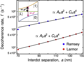
Figure 3. Dependence of the phonon-induced decoherence rates on interdot separation for the Larmor (red) and Ramsey (blue) pulse sequences, keeping the tunnel coupling fixed at t = −8.2 μeV. The decoherence rates grow with a because the same long wavelength phonon causes a larger distortion of the triple dot. The specific dependences of decoherence rates on a, for the dominant  and
and  decoherence processes shown in the inset, are given by a2 and a4, respectively. We therefore fit the data to the form shown in the figure, yielding the fitting coefficients A3 = 1.33, C3 = 0.000 077, A4 = 25.52, and C4 = 0.000 255. Here, l = 18.5 nm and T = 50 mK.
Download figure:
Standard image High-resolution imageIt is possible to tune the phonon-induced decoherence rates by modifying geometrical device parameters. The dependence of ΓLar and ΓRam on interdot distance is shown in figure 3. Here, we tune a while holding the tunnel coupling t = −8.2 μeV constant; experimentally this can be accomplished by varying gate voltages. We take l = 18.5 nm for all points here, to consider solely effects of changing a. Figure 3 shows that the rates grow with a as a linear combination of power laws a2 and a4, which is justified by expanding the functions J1L and J10 in small values of their exponential arguments. For ΓRam this expansion is not strictly valid, however we find that a fit with the same power laws seems to work. The physics underlying the growth of ΓLar and ΓRam with a is that the decoherence is dominated by phonons with wavelengths larger than the triple dot size; as the QD separations are increased, the phonon causes larger shifts within the triple QD, and consequently more decoherence.
The temperature dependence of the decoherence rates is shown in figure 4. Both rates grow very slowly with temperature up until about 0.1 K, particularly ΓRam, and then increase linearly with T at higher temperatures. The linear dependence on temperature appears when  , causing the Bose–Einstein distribution to reduce to a classical distribution. The transition occurs at lower temperatures for ΓLar than for ΓRam, because the Larmor pulse sequence involves smaller energy splittings than the Ramsey sequence.
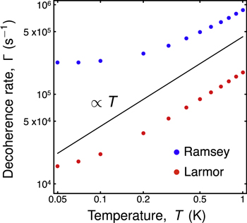
Figure 4. Temperature dependence of the phonon-induced decoherence rates for Larmor (red) and Ramsey (blue) pulse sequences, at t = −8.2 μeV, l = 18.5 nm, and a = 90 nm. The black line serves as a guide to indicate the dependence proportional to temperature. The transition to the linear regime occurs at lower temperatures for the Larmor pulse sequence, because the relevant energy scales are smaller than those of the Ramsey sequence, as indicated in figure 1(d). Consequently, a high-temperature expansion of the Bose–Einstein distribution is valid at lower temperatures for the Larmor sequence, than for the Ramsey sequence.
Download figure:
Standard image High-resolution image5. Qubit fidelity
One of the main questions to be answered in this work is whether phonon-mediated noise presents a challenge for charge quadrupole qubits, and how phonon-induced decoherence compares to decoherence from charge noise, which was studied in [31, 32]. Similar to [32], we assume the charge noise to be quasistatic, with fluctuations of the dipolar detuning parameter that follow a Gaussian distribution with a standard deviation of 1 μeV [58], as typical for experiments. A composite  pulse sequence was implemented, to eliminate the effects of leakage to leading order, and the average gate fidelity was calculated as described in [32]. The pulse sequence used in these simulations is shown in figure 6, with additional details given in appendix G. For the phonon noise, we use the same pulse sequence. However, we modified the Ramsey sequence in figure 5 by setting t = 0 during the Z rotation, as proposed in [32]. This has the benefit of suppressing the phonon-induced tunneling during Ramsey oscillations, so that decoherence occurs only during Larmor precession. To compute the average gate fidelity for phonon-induced noise during the free evolution portion of the Larmor sequence, Fph, we average over initial states using the standard definition
  . Here, ξ are indices denoting the initial states that form a regular tetrahedron on the Bloch sphere [59], and
  is a density matrix for the ideal system, i.e. without phonons.
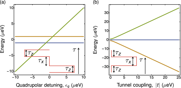
Figure 5. The pulse sequence used in the infidelity calculations of figure 6 (vertical axis is time), and the energy spectrum of the three-level system described by the Hamiltonian shown in equation (5) for (a) t = 0, d = 1 μeV and (b) q = 0, d = 1 μeV. As indicated, the system evolves for time τz with zero tunnel coupling t and non-zero quadrupolar detuning q, and for time τx with non-zero t and zero q. This specific pulse sequence was proposed in [32] to suppress leakage to state  caused by quasistatic charge noise. Here, the quasistatic charge noise is represented by non-zero d.
Download figure:
Standard image High-resolution imageResults of our calculations are shown in figure 6 for decoherence from both phonons and charge noise. For phonons, the infidelity increases with  , for the same reason as in figure 2. For charge noise, the fidelity shows the opposite trend, due to the suppression of leakage for large
  , and the broadening of the charge noise sweet spot, which is used to suppress decoherence in the quadrupole qubit [31]. As a result, an optimal working point emerges near t ≃ 17 μeV, corresponding to a maximum fidelity >99.99%.
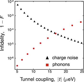
Figure 6. Average gate infidelity 1 − F of the free evolution portion of the Larmor pulse sequence (red squares), computed in the presence of phonons. The infidelity grows with  , so high-fidelity operations can be achieved only when
  is not too large. The charge noise-induced infidelity (black triangles), calculated as in [32], shows the opposite trend with
  . Considering both noise processes, an optimal working point emerges at
  . Here, as well as for figure 2, the interdot separation is a = 90 nm, the dot size l is determined transcendentally from equation (6), and T = 50 mK.
Download figure:
Standard image High-resolution image6. Discussion
In this work, we have considered phonon-induced decoherence of a charge quadrupole qubit to determine its optimal working regime. We find that decoherence rates increase quickly with energy level splitting, due to the strong dependence of the phonon density of states and electron–phonon interaction matrix elements on it. This suggests that large tunnel couplings and quadrupolar detunings should be avoided during qubit operation. However, decoherence caused by charge noise is found to decrease rapidly as the tunnel coupling is increased, due to the suppression of leakage and broadening of the sweet spot. Hence an optimal working point emerges for the tunnel coupling, which we estimate to be t ≃ 17 μeV for typical devices, corresponding to average gate fidelities greater than 99.99%, with X gate periods of 0.13 ns and Z gate periods of 0.055 ns. We also find that smaller dot separations tend to reduce the phonon-induced decoherence; a similar trend was previously observed for the coupling to charge noise [31].
Our calculations here focus on the effects of phonons and charge noise within the three-level system  , and we do not explicitly consider other possible sources of decoherence. For example, we do not consider the presence of non-qubit excited states (other than
  ), which can provide additional leakage channels when their energy splittings are comparable to the qubit energy. In Si heterostructures, these can include both excited orbital and valley states [60]. To quantify such effects, we note that the orbital excitation energies of the dots considered in this work is > 0.83 meV, while the reported values of valley splittings in similar QDs can be ∼0.12 meV in Si/SiGe heterostructures [61, 62] and 0.3–0.8 meV in Si/SiO2 heterostructures [63, 64]. In comparison, for the phonon-induced decoherence the largest energy splitting considered here was ∼0.1 meV, while at the optimal working point shown in figure 6, the largest energy splitting was 0.048 meV. For the temperatures usually used for such devices (<100 mK), the dominant phonon-induced decoherence processes are
  and
and  , accompanied by the emission of a phonon. Compared to these, the transition processes involving absorption of a phonon,
  and
and  , are strongly suppressed because their transition rates are proportional to the Bose–Einstein distribution function,
 ![${n}_{{\rm{BE}}}=1/(\exp [{\hslash }{\omega }_{{\bf{q}}s}/({k}_{B}T)]-1)$](https://content.cld.iop.org/journals/1367-2630/20/10/103048/revision2/njpaae61fieqn120.gif) , while emission rates are proportional to
, while emission rates are proportional to  , which is exponentially larger than nBE. For more details about transition rates see appendix F. Therefore, transitions to even higher energy states are strongly suppressed and can be neglected. However, in some situations, the excited states could lie closer to the qubit subspace, in which case the absorption of a phonon could cause leakage that suppresses the qubit fidelity.
Another source of infidelity not considered in this paper is the possible population of highly excited states due to the non-adiabatic nature of sudden gate pulses. However, infidelity arising from this source can be suppressed greatly by application of shaped pulses, as discussed in [65–67].
7. Conclusions
In conclusion, we have studied the effects of phonons on the coherence of a charge quadrupole qubit. Our results suggest that phonons can be a dominating source of decoherence in some regimes and should be taken into account if a qubit with this architecture is realized experimentally. We show, however, that there are also regimes, where the combined effects of phonons and quasistatic charge noise lead to qubit infidelities less than 0.01%.
Acknowledgments
We thank Mark Eriksson, Joydip Ghosh, and Zhenyi Qi for helpful discussions. This work was supported in part by ARO (W911NF-15-1-0248, W911NF-17-1-0274) and the Vannevar Bush Faculty Fellowship program sponsored by the Basic Research Office of the Assistant Secretary of Defense for Research and Engineering and funded by the Office of Naval Research through Grant No. N00014-15-1-0029. The views and conclusions contained here are those of the authors and should not be interpreted as representing the official policies, either expressed or implied, of the Army Research Office (ARO), or the US Government.
Appendix A.: The wave function of an electron in the heterostructure growth direction
The full wave function of an electron in a triple QD can be represented as a product of a component in the direction of heterostructure growth (z) and a lateral component (x − y), because the confinement potential can be approximated as a sum of z and x − y terms. The lateral components of the wave functions ψ(x, y) are discussed in the main text. Here we summarize our treatment of the z component φ(z). Taking into account both subband and valley physics, a convenient approximate expression for the wave function of an electron in the direction of quantum well confinement is (see e.g., [43, 68])

where k0 is a wave vector corresponding to the 'valley' minima of the conduction band in Si,  , with the length of the Si cubic cell a0 = 0.54 nm. The parameter d defines the width of the quantum confinement. As d is typically < 10 nm, the wavelengths of the relevant phonons are much larger than d. Therefore the effect of phonons in the z direction is approximately a constant shift of atoms, and the contribution from the z dimension to the electron–phonon interaction matrix element
  , where z0 is a point near the wave function maximum. Consequently, the contribution from the z dimension to the decoherence rates is roughly the same for any approximation of φ. Therefore in our calculations we further simplify φ as follows:

Through numerical simulations we have verified that this simplification does not noticeably affect the results obtained in our Fermi Golden rule calculations, and therefore we believe that it also does not affect the results of the Bloch–Redfield formalism.
Appendix B.: Derivation of the wave functions of an electron in a triple QD
As described in section 2, the wave functions of an electron in a triple QD ΦL, ΦC, and ΦR are constructed from the harmonic oscillators ground states ψL, ψC, and ψR using a well known procedure described in [47, 48]. We first define the overlap integral  . Taking into account that
  due to the large distance between left and right dots, we express the electron wave functions in terms of linear combinations of ψL, ψC, and ψR as follows


and then determine g1, g2,  , and
, and  by solving the conditions for orthogonalization and normalization of ΦL, ΦC, and ΦR, which are


These conditions yield two solutions. The first solution, g1 = 0 and g2 = S, corresponds to localized basis states for the left and right dots, and a delocalized basis state for the center dot. The second solution, which is used in this work, is given by  and
and  (for this solution,
  and
and  ). The latter appears more physical than the first solution because it treats the three dots on an equal footing by introducing a small amount of delocalization in each case. It also appears more analogous to the basis states used in the analysis of double QDs [47]. It would be interesting to compare how these different solutions affect our final results; however, we have not done so here.
Appendix C.: Tunnel coupling
From equation (5) in the main text, the definition of tunnel coupling is  . We evaluate t by considering the tunneling of a particle in a double-well potential given by
  . This potential includes only two quantum wells, but this is sufficient for our purposes because the third dot is far away, and its effect is exponentially suppressed. To evaluate t we use the wave functions constructed similarly to ΦR and ΦC, namely[47, 48]


where  are the same as for the x-components of
  in the main text, but shifted along x by a/2, rather than a. Consequently, the formula for the tunnel coupling becomes
  . Then the expression for t is

The rapid growth of t with l arises because  .
.
We note that as  and
and  contain ψC, there is the tunneling term between them
  . In the parameter regime we consider here, its effect on the spectrum is not significant and will not lead to a noticeable change in phonon-induced decoherence processes.
Appendix D.: The electron–phonon interaction Hamiltonian
In this appendix we present a detailed expression for the electron–phonon Hamiltonian in bulk Si; it is given by [50]

where  is a strain tensor defined as [45, 51]


where Ξd and Ξu are deformation potential constants,  is a displacement operator,
  (corresponding to one longitudinal and two transverse acoustic modes), vs is the speed of sound for each of these modes, ρSi is the mass density of bulk Si, V is the volume we consider,
  and
and  are annihilation and creation operators for phonons of mode s and wave vector
  . The polarization vectors are chosen as follows:
  ,
,  and
and  leading to the definition
  ,
,  , and
, and  . The explicit expressions for polarizations are

where  and
and  are angles describing the phonon wave vector
  in spherical coordinates
  . Writing equation (D.1) in a more explicit form, we get
As the  matrix elements will be important below, particularly
  and
and  , we present their explicit forms here:
Appendix E.: Bloch–Redfield Formalism
Here we derive the equation for the reduced density matrix that describes our three-level system, which we use to obtain decoherence rates from the decay of the occupation of the system's states. We follow the standard procedure for deriving Bloch equations [39, 54, 69].
The Hamiltonian in our problem is given by

where Hq is the Hamiltonian of a qubit (including the leakage state in our case), Hph describes the Hamiltonian of the phonons and  is an interaction between them. The von Neumann equation for the full density matrix in the Schrödinger representation is given by

where we set ℏ = 1 for brevity. In the interaction representation defined as  , the von Neumann equation becomes

and integration yields

Substituting into equation (E.3) yields

As we are mainly interested in the three-level system of the qubit with the leakage state, we trace over phonon degrees of freedom to obtain the reduced density matrix:

We then apply the Born approximation:  and the Markov approximation
  inside the integral. Here we note that
 ![${{\rm{Tr}}}_{{\rm{ph}}}\{[{\rho }_{{\rm{int}}}^{{\rm{ph}}}(0)\otimes {\rho }_{{\rm{int}}}^{q}(0),{H}_{q-{\rm{ph}}}^{{\rm{int}}}(t)]\}=0$](https://content.cld.iop.org/journals/1367-2630/20/10/103048/revision2/njpaae61fieqn164.gif) because
because  , and similarly for
  . Therefore only the first term remains in equation (E.6), which after the Born–Markov approximations reads

We expand the commutator to obtain

We then project this equation onto the qubit-leakage basis (dropping the notation 'int' for brevity), yielding:
where the convention of summing over repeated indices is used. We also switch to a different interaction picture in the following way:

where the bar denotes the interaction representation with respect to the phonon Hamiltonian only, and  , where En and Ek are the energies of states n and k, respectively. We apply such representation to all the Hamiltonian terms in equation (E.9), obtaining
We make the substitution  , obtaining
Defining


our equation takes the form

Note, that we omitted the superscript 'int' here to simplify the notation; however the reduced density matrix is in interaction representation as shown above in equation (E.3). To transform back to the Schrödinger representation we use


Finally, in the Schrödinger representation, we obtain

Here, the initial conditions are defined by the desired pulse sequence, as discussed in the main text and figure 1(d). By computing the density matrix as a function of time for a particular initial condition, we can determine the decoherence rates by fitting the decay of the measured state to the exponential form  .
.
Appendix F.: Fermi Golden rule calculation of transition rates
In this section we use Fermi Golden rule to calculate the transition rates of the relaxation processes between different states. These rates have similar form to equations (E.13) and (E.14), which helps us to better understand the behavior of results obtained from the Bloch–Redfield formalism. We assume that the initial state is one of the qubit states.
The Fermi Golden rule expression for the transition rate from initial state  to final state
  is
is

where − corresponds to absorption and + corresponds to emission of a phonon,  , and the initial and final states
  and
and  , respectively, describe both the electron and the phonon bath. Here, the initial and final energies of the electron are Ei and Ef, and the frequency
  corresponds to a phonon that is emitted or absorbed.
The full expressions for the rates are lengthy, therefore we do not include them all here. However we provide one of the shortest of the expressions as an example:
where  , nBE is the Bose–Einstein distribution function, and
  is defined in terms of the electron–phonon matrix elements as follows:
The relaxation rates are calculated for the following set of Si material parameters: deformation potential constants Ξd = 5 eV, Ξu = 8.77 eV, longitudinal speed of sound  m s−1, transverse speed of sound
  m s−1, and mass density
  . The quantum confinement in the z direction is characterized by d = 2 nm, as defined in equation (A.2).
Since we consider the low temperature T = 0.05 K, as consistent with QD experiments performed in a dilution refrigerator, the phonon absorption rates are much slower than emission rates. Mathematically this follows from the fact that emission rates have a nBE + 1 term, as in the last bracket of equation (F.2), while absorption rates only have nBE. Therefore, since nBE becomes very small for low temperatures, emission rates dominate over absorption. These are given by Γ10 between the qubit states  and
and  , and
, and  between the states
  and
and  , as depicted in figure F1.

Figure F1. Dependence of the energies of  ,
,  , and
, and  states on quadrupolar detuning q. Arrows show all possible one-phonon relaxation processes, where Γ10 and
  are found to be dominant.
Download figure:
Standard image High-resolution imageWhen q = 0 the main contribution to  in the parameters ranges we consider, comes from the difference
  , appearing in equation (D.8). Similarly, for Γ10, the main contribution comes from the combination
  , appearing in equation (D.9), for nearly all the parameter ranges considered here. The rates
  and Γ10 for q = 0 can be approximated as follows


Here, a factor of  comes from the phonon density of states, another factor of
  comes from the form of the electron–phonon interaction and the exponential terms describe the phase shifts between matrix elements PLL, PCC, and PRR due to the interdot separation a. The transverse phonons dominate for these parameters, therefore the approximation with only
  works well. Following the fact that the relaxation processes
  and
and  are dominating in the decoherence rates for Larmor and Ramsey pulse sequences, we used J1L and J10 to fit the results for the dependences of the decoherence rates on
  and a for figures 2 and 3.
As the dots are gate-defined, the size of each dot can be varied. Here, the transverse size of the dots is characterized by l. Since the experimentally relevant quantity is the tunnel coupling, here we present the dependence of Γ10 and  on
on  , whereas t is calculated using geometrical parameters a and l of the triple QD, see figure F2. When
  , we can expand the exponents in equation (F.4), obtaining the power law
  , whereas for equation (F.5), when
  , we get the power law
  .
.
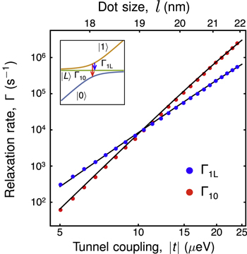
Figure F2. Dependence of the relaxation rates Γ10 and  at q = 0 on the absolute value of the tunnel coupling
  . The values of the QD size, l, are related to
  through equation (6), as shown on the top axis. The black lines are fit of
  to
to  and for Γ10 to ∝J10. The inset shows the relaxation processes that give rise to Γ10 and
  on the energy level diagram. Both relaxation rates increase strongly with
  . Here, we assume an interdot separation a = 90 nm, and a temperature T = 50 mK.
Download figure:
Standard image High-resolution imageAnother geometrical parameter we consider is the interdot separation a. We plot the dependence of  and Γ10 on a in figure F3 for q = 0 and q = 30 μeV. We see that Γ10 and
  are both more than ≃10 times smaller for q = 0 than for q = 30 μeV. In the former case we find that the rates depend on interdot distance a as
  and
and  , with very good precision for all a in
  and for a > 80 nm in Γ10. This behavior arises from the exponential terms in equations (F.4) and (F.5), which can be expanded to give the power laws a2 and a4 in the leading order. The behavior of Γ10 for a < 80 nm can be explained as follows. The overlap between wave functions becomes strong enough to cause the off-diagonal matrix elements PLC, PCR,
  , and
, and  to contribute significantly to the relaxation rate, therefore modifying the power law. Note that when q = 30 μeV, the arguments of the exponential factors in equations (F.4) and (F.5) are not small for part of the parameter range, so the expansion is no longer valid.

Figure F3. Dependence of the relaxation rates Γ10 and  on the interdot separation a for quadrupolar detuning q = 0 (lower two curves) and q = 30 μeV (upper two curves). In general, the rates grow with a because as the distance between the dots increases, the phase difference of the phonon wave in the different dots increases. Consequently, the phonons give rise to larger distortions of the triple QD potential. Here, the size of the dots is l = 18.5 nm, tunnel coupling t = −8.2 μeV, and temperature T = 50 mK.
Download figure:
Standard image High-resolution imageThe increase of the relaxation rates with a can be explained physically as follows. Phonons induce transitions by perturbing the triple dot potential, as schematically depicted in figure 1(c). Since the phonons responsible for the transitions are long-wavelength, if the triple QD has small dimensions, it experiences the phonon as an approximately uniform shift in energy. If the dots are further apart, the same phonon produces larger shifts between the dots, appearing in the  matrix elements, which consequently produces more relaxation.
The dependence of  and Γ10 on quadrupolar detuning is determined by the energy level spacing between the states we consider. As figure F4 shows, the rate Γ10 is at a minimum when the energy splitting between
  and
and  is at a minimum (q = 0) and exhibits symmetric behavior about q = 0, as depicted in the inset. In contrast, the energy splitting between
  and
and  is asymmetric along the q axis, yielding an asymmetric dependence of
  on q. We also present in figures F5 and F6 the contour plots for the dependences of Γ10 and
  on
on  and q.

Figure F4. Dependence of the relaxation rates Γ10 and  on the quadrupolar detuning q. The dependence of Γ10 exhibits symmetric behavior as the qubit energy splitting is also symmetric with respect to q = 0, as shown in the inset. The splitting between
  and
and  is very small when q is large and negative; consequently
  is very small in this regime. For qubit operation, both relaxation rates should be small, so operation near q = 0 is expected to yield the best results. Here, the set of parameters is the same as for figure F3 and the interdot separation a = 90 nm.
Download figure:
Standard image High-resolution image
Figure F5. Dependence of the relaxation rate Γ10 on the quadrupolar detuning q and tunnel coupling magnitude  , exhibiting symmetric behavior similar to figure F4. Here, the interdot separation a = 90 nm, temperature T = 50 mK, and l depends on t, as per equation (6).
Download figure:
Standard image High-resolution image
Figure F6. Dependence of the relaxation rate  on the quadrupolar detuning q and tunnel coupling magnitude
  , exhibiting asymmetric behavior similar to figure F4. The dot parameters used here are the same as for figure F5.
Download figure:
Standard image High-resolution image
Appendix G.: Charge noise-induced infidelity
In this section we present the model we used to calculate quasistatic charge noise-induced infidelity for the charge quadrupole qubit. To find an optimal working point for the charge quadrupole qubit, we considered pulse sequences that reduce leakage effects caused by charge noise, as described in [32]. Following the procedure from [32], we first define

in the basis

where  and
and  correspond to logical states and
  is a leakage state. Here d represents the charge noise on the gates; we take it to be d = 1 μeV [58]. The operators that generate Z and X rotations, including charge noise, are defined as follows


for the rotation angles ϕ and θ. We define gate times using ϕ and θ as  and
and  , which correspond to the case of absence of charge noise. From equation (G.3) follows that during Z rotation we set t to zero.
To construct an effective, leakage-suppressed X(π) rotation, we apply the pulse sequence

and take ϕ = 2π, θ = 3π, and  , which is equivalent to
  in the absence of charge noise. We then define the operation W to be the projection of
  onto the 2D logical space [70]. The definition of the average gate fidelity is then

where the desired gate operation, Wtarget = X(π), is in 2D logical space, and D = 2.