

Abstract
Land surface phenology (LSP) derived from satellite data has been widely associated with recent global climate change. However, LSP is frequently influenced by land disturbances, which significantly limits our understanding of the phenological trends driven by climate change. Because wildfire is one of the most significant disturbance agents, we investigated the influences of wildfire on the start of growing season (SOS) and the interannual trends of SOS in the Hayman Fire area that occurred in 2002 in Colorado using time series of daily MODIS data (2001–2014). Results show that the Hayman Fire advanced the area-integrated SOS by 15.2 d and converted SOS from a delaying trend of 3.9 d/decade to an advancing trend of −1.9 d/decade during 2001–2014. The fire impacts on SOS increased from low burn severity to high burn severity. Moreover, the rate of increase of annual maximum and minimum EVI2 from 2003–2014 reflects that vegetation greenness could recover to pre-fire status in 2022 and 2053, respectively, which suggests that the fire impacts on the satellite-derived SOS variability and the interannual trends should continue in the next few decades.
Export citation and abstract BibTeX RIS

Original content from this work may be used under the terms of the Creative Commons Attribution 3.0 licence.
Any further distribution of this work must maintain attribution to the author(s) and the title of the work, journal citation and DOI.
1. Introduction
Vegetation phenology, characterizing both physical changes (e.g. leaf development and abscission) in vegetation structure and the inherent seasonality of mass and energy flux, is considered to be a crucial regulator of ecosystem processes and feedbacks to climate (Gu et al 2003, Richardson et al 2012), as well as a sensitive bioindicator of monitoring climate change and carbon cycle (Richardson et al 2013). In recent years, growing evidence has emerged that climate change is altering phenological variation in terrestrial ecosystems across scales from individual species to landscapes (Schwartz et al 2006, Richardson et al 2013, Angert et al 2005). As a result, vegetation phenology has been selected as one of the most effective and simplest indicators to track changes in the ecology of species in response to climate change (Pachauri et al 2014) and is listed as one of the leading indicators of climate change identified by the United States (US) Global Change Research Program (www.globalchange.gov/) and US Environmental Protection Agency (EPA) (www.epa.gov/climate-indicators).
Satellite data have been widely recognized as a powerful tool in identifying spatially distributed phenological indicators of climate change. Specifically, the start of growing season (SOS) has been extensively derived from the Advanced Very High Resolution Radiometer (AVHRR) Normalized Difference Vegetation Index (NDVI) data, which have been available since 1981, based on various approaches and time periods (Reed et al 1994, White et al 2009, de Beurs and Henebry 2005b, Zhang et al 2007, Zhou et al 2001, de Jong et al 2011). The interannual SOS trend has been widely used to associate with regional or global climate change although the magnitude and direction of SOS trends varied greatly in different locations, time periods, spatial and temporal scales, and measuring methods (Walther 2004, Jeong et al 2011, Zhang et al 2007, Zhou et al 2001, Shen et al 2014).
Unlike the field observations of species-specific phenology, land surface phenology (LSP) is commonly used to refer to the area-integrated phenology of vegetation communities detected from satellite remote sensing (de Beurs and Henebry 2004). Within a satellite pixel, land surface components and plant species composite may be strongly altered by land disturbances. This could lead to a great change of phenological timing within a satellite pixel and may in turn significantly modify the direction and magnitude of the interannual phenological trend. It is very likely that current detections of LSP indicators can be strongly influenced by land use, disturbance history, and human activity (Buyantuyev and Wu 2012, de Beurs and Henebry 2004, Romo-Leon et al 2016, White et al 2005). This issue severely limits our understanding of phenological variability and trends reflecting climate change across regional to global scales (White et al 2005). Thus, it is necessary to separate the abrupt change caused by land disturbance from the gradual change associated with climate change (Verbesselt et al 2010).
Wildfire is one of the most important drivers of land disturbances across the world. Because fire size, severity and frequency have been increasing in many parts of the world during past decades (Pechony and Shindell 2010, Westerling et al 2006, Marlon et al 2012), the impacts of wildfires on the changes of land cover types and soil properties (such as nutrients and water availability) have likely increased (Miller et al 2013). Although some studies demonstrated the post-fire LSP variation (Van Leeuwen et al 2010, van Leeuwen 2008, Sankey et al 2013, Fernandez-Manso et al 2016, Storey et al 2016, Di-Mauro et al 2014), however, the quantitative impact of wildfire on LSP and its interannual trend has been barely investigated and remains poorly understood.
This study aims to quantitatively explore the impact of wildfire on interannual LSP trend. Specifically, we detected LSP around the Hayman Fire in the central United States using a time series of daily Moderate-resolution Imaging Spectroradiometer (MODIS) data from 2001–2014. We further quantified the difference between pre-fire and post-fire LSP for the areas with different levels of burn severity and calculated the LSP trends inside and outside the burn scar, with which the wildfire influence on LSP was explored.
2. Methodology
2.1. Burn severity and land cover data
The Hayman Fire, which started on June 8 and ended on July 18, 2002, in Colorado's Front Range (39°13'12.0''N, 105°17' 13.2''W; see figure 1(a)), was the largest wildfire in the recorded history of Colorado with a burned area of 526 km2. We obtained the burned area and burn severity levels from the Monitoring Trends in Burn Severity (MTBS; www.mtbs.gov) map. These data were generated by comparing the pre-fire and post-fire Normalized Burn Ratio (NBR) derived from Landsat data at a 30 m resolution (Eidenshink et al 2007). Burn severity represents primarily the effect of fire on vegetation biomass levels, which is classified as the categories of unburned to low, low, moderate, high, and increased greenness. Areas affected by clouds, cloud shadows, and data gaps are labeled as non-processing. To match the LSP map (see subsection 2.2), the burn severity map was resampled to 240 m based on the majority of burn severity levels. The upscaled burn severity map contains 52.1% of high severity, 17.5% of moderate severity, 4.3% of low severity, 2.5% of unburned to low, 0.7% of non-processing, and no area of increased greenness (figure 1(b)). The pixels with non-processing were excluded for further analyses because of limited coverage. To investigate the wildfire impact on LSP, we set up a buffer zone of 5 km outside the burn scar as a reference representing the area without disturbances.
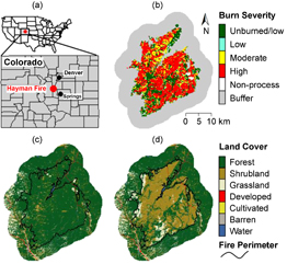
Figure 1 The location of the Hayman Fire (a), burn severity map (grey is the buffer zone with a width of 5 km used as an unburned reference) resampled to 240 m (b), and National Land Cover Database maps in 2001 (c) and 2006 (d) at 30 m resolution.
Download figure:
Standard image High-resolution imageNational Land Cover Database (NLCD; can be found in www.mrlc.gov) data in 2001, 2006 and 2011 were acquired to analyze the change of land cover types, which were before (in 2001) and after (in 2006 and 2011) the fire occurrence. The NLCD maps were produced using Landsat data with a spatial resolution of 30 m (Homer et al 2015, Fry et al 2011, Homer et al 2007). The NLCD land cover was reclassified into seven types that are forest, shrubland, grassland, developed land, cultivated land, barren, and water (figure 1). NLCD 2011 was not shown here because the land cover type was almost the same as that in 2006 in our study region. Before the fire occurrence, forests were dominant, which mainly consisted of evergreen forests (mainly ponderosa pine–Douglas fir forest) with small proportions of deciduous and mixed forest (<2%) and a few scattered shrub patches. After the fire occurrence, the forests were mainly converted to shrublands with a small portion of grasslands around the burn perimeter, but some forests remained unchanged after the fire. The unchanged forests were mainly located in the areas with unburned/low and low burn severity, while the land cover conversions generally occurred in the areas with moderate and high burn severity. The proportion of 30 m land cover in each 240 m grid of the upscaled burn severity map was further calculated and averaged based on the burn severity levels to quantify the burn severity influence on land cover conversion.
2.2. Phenology detection from satellite data
To detect LSP in the Hayman Fire area, we first collected daily MODIS surface reflectance products (MOD09GQ, V006) in tile H09V05 at a spatial resolution of 250 m from 2001–2014. Reflectances at red and near-infrared bands in MOD09GQ were used to calculate daily two-band enhanced vegetation index (EVI2), which is equivalent to EVI (Jiang et al 2008). Compared with NDVI which combines reflectances at near-infrared and red bands to reflect vegetation greenness, EVI is developed by adding the blue band and other adjustment coefficients so that it is less sensitive to soil background brightness and atmospheric scattering contamination and does not saturate over high densely-vegetated areas (Huete et al 2002). After replacing the blue band (relatively low signal-to-noise ratio) using the auto-correlative properties of surface reflectance between the red and blue bands, EVI is modified to EVI2 that remains the advantages over NDVI (Jiang et al 2008). Further, MODIS land surface temperature (LST) products (MOD11A1, V005) and daily surface reflectance products (MOD09GA, V006) at a spatial resolution of 1 km were also collected for extracting LST and cloud and snow flags, respectively. The LST and cloud and snow flag data were simply downscaled to 250 m using a nearest neighbor approach. Because of missing MODIS data in early 2000 (1/1/2000–2/23/2000) and in June 2002, which severely impaired the accuracy of LSP detection, our study period was set to be 2001 (pre-fire) and 2003–2014 (post-fire), which was simply called as 2001–2014 hereafter.
The hybrid piecewise-logistic-model-based LSP detection algorithm (HPLM-LPSD) was applied to retrieve the LSP metrics from the time series of daily EVI2 (Zhang et al 2003, Zhang 2015). There were mainly five steps in implementing HPLM-LPSD to retrieve phenological metrics for a target year: (1) establishment of a three-day EVI2 time series composited by selecting good quality observations, (2) determination of background EVI2 by calculating the mean of the 10% largest EVI2 values with cloud- and snow-free observations during a winter period defined using LST <278 K (during the dormancy phase), (3) smoothing of the EVI2 time series by removing the local sharp peak or trough with a Savitzky–Golay filter and a running local median filter, (4) reconstruction of the EVI2 time series using the hybrid piecewise logistic functions, and (5) detection of the phenological transition dates by identifying the day of year (DOY) which shows the maximal or minimal rate of change in the curvature along the reconstructed EVI2 time series. The temporal EVI2 observations and phenology detection were illustrated in figure 2.
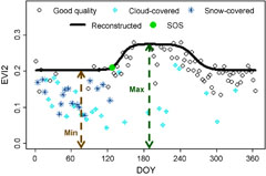
Figure 2 An example of reconstructing temporal vegetative EVI2 trajectory and detecting SOS, minimum EVI2 (Min), and maximum EVI2 (Max) using HPLM-LPSD. Note that fill values (invalid observation in MOD09GQ) are not presented. The irregular variation in good quality EVI2 is likely associated with the residual cloud contamination and bidirectional reflectance distribution function.
Download figure:
Standard image High-resolution imageThe confidence of phenology detections was quantified using the proportion of good quality (cloud- and snow-free) EVI2 (PGQSOS) around the SOS occurrence (Zhang 2015, Zhang et al 2009). To ensure the reliability of SOS detections, a filter of PGQSOS >40% was applied to select high confidence SOS pixels.
In addition, the annual maximum and minimum EVI2 were also derived from the EVI2 time series reconstructed based on the hybrid piecewise logistic model. The minimum EVI2 is usually the background EVI2 during a winter period determined in step 2 of HPLM-LPSD. The resultant metrics were then resampled to 240 m using the nearest neighbor method.
2.3. Investigation of wildfire impacts on SOS
The impact of wildfire on SOS was quantitatively analyzed using two parameters. First, spatial SOS anomaly was calculated by comparing the SOS values inside the burn scar with those in the buffer zone (as a reference) outside the burn scar for individual years.

where SOSi,y and SOSo,y are the area-integrated SOS (median of SOSs) inside the burn scar and in the buffer zone for year y, respectively, and SOSa,y is the spatial SOS anomaly in year y. As the pre-fire record is only available in 2001, SOSa,2001 was used as the pre-fire measurement. The average spatial anomaly from 2003–2014 was used as the post-fire measurement. The spatial pattern of SOS anomalies in pre-fire and post-fire was further compared.
Second, SOS trends were examined and compared for overall areas inside the burn scar and in the buffer zone and for individual pixels, respectively. Overall trends were determined from the time series of SOS during 2001–2014 inside the burn scar (SOSi,y) and in the buffer zone (SOSo,y), separately. The trends for individual pixels were also calculated with a simple linear regression to evaluate the detailed spatial variations. The significance of the trends was determined using the single tailed student's t-test. Note only the pixels (2174 inside the burn scar and 2317 in the buffer) with valid SOS detections (PGQSOS > 40%) for the entire study period (2001–2014) were included for the trend analysis.
3. Results
3.1. Land cover change by wildfire and post-fire vegetation recovery
Figure 3 presents the comparisons of proportions of 30 m land cover in each 240 m pixel before and after the fire occurrence. This result, to some extent, indicated the land cover changes by wildfire burning with different severity levels. In the entire study area, natural vegetation (forests, shrublands and grasslands) accounted for more than 97% on average. In the buffer zone, the proportion of forests, shrublands, and grasslands was 80%, 9% and 8%, respectively, with little difference between pre-fire and post-fire periods. In the burn scar, the proportion of forests, shrublands, grasslands was 90%, 7%, and 2% in 2001 and 30%, 60%, and 8% in 2006 and 2011, respectively. While evergreen and deciduous shrubs were not separated in shrublands, the forests were mainly evergreen, among which deciduous and mixed forests only accounted for 1.61% in 2001 and 1.14% in 2006 and 2011. The forest proportion before the fire event was large in the regions with high burn severity while small in the low burn severity, indicating that the regions with more forests tended to be burned more severely. The forest proportion after fire occurrence decreased while the shrubland and grassland proportion increased with the burn severity level, indicating that higher burn severity caused more forests converted to shrublands and grasslands. The land cover proportions in 2011 were almost the same as those in 2006.
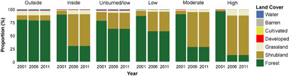
Figure 3 The proportion of 30 m land cover in each 240 m pixel in 2001, 2006, and 2011 at different burn severity levels derived from NLCD maps (Outside is the buffer zone, Inside is the entire burn scar, and Unburned/low, Low, Moderate, and High represent different levels of burn severity).
Download figure:
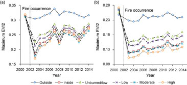
Standard image High-resolution imageFigure 4 displays variations of annual maximum and minimum EVI2 values to demonstrate vegetation recovery through the post-fire period (2003–2014). The annual maximum EVI2 represented the overall vegetation growth in the Hayman Fire because almost all the plants reached their peaks during summer. In contrast, the annual minimum EVI2 revealed the recovery of evergreen plants because there were no green leaves on deciduous plants during winter. In 2001, the annual maximum and minimum EVI2 values inside the burn scar and in the buffer zone were very similar, demonstrating that their vegetation growing conditions were almost identical across the region before fire occurrence. The slight divergences appeared in the minimum EVI2, which might be caused by the variation in proportion of evergreen and deciduous plants. After the occurrence of the Hayman Fire in 2002, both maximum and minimum EVI2 values inside the burn scar dropped sharply but basically remained stable in the buffer zone. In the post-fire period (2003–2014), the EVI2 inside the burn scar showed increasing trend, as the vegetation recovering and non-native plants invading. The rate of increase on average was 0.052 per decade in the maximum EVI2 and 0.029 per decade in the minimum EVI2. These rates reflected the recovery of total vegetation and evergreen trees, separately. The increase rate in EVI2s was similar across the areas with different levels of burn severity although the magnitude of EVI2 values varied. Based on the current recovery rates, the annual maximum and minimum EVI2 and would reach pre-fire status in 2025 and 2053, respectively.

Figure 4 The spatially-averaged annual EVI2 time series with different burn severity levels from 2001 to 2014: annual maximum EVI2 (a) and annual minimum EVI2 (b) in the buffer zone (Outside) and inside the burn scar (Unburned/low, Low, Moderate, and High are the EVI2 with different burn severity levels and Inside is the EVI2 in the entire burn scar).
Download figure:
Standard image High-resolution image3.2. Impacts of fire on SOS in different levels of burn severity
Figure 5 displays the spatial distributions of SOS around the Hayman Fire in one year before (2001) and after (2003) the fire occurrence. For the proper comparison, the SOS dates only represent the pixels with high confidence, which varied spatially from 40 to 200 DOY. In both years, the southern and eastern regions tended to have later SOS dates, compared to the western and central parts. In the buffer zone, SOS was relatively stable from 2001 to 2003, although it was later in the west and east regions and earlier in the north and southeast. Inside the burn scar, SOS dates were generally advanced, except for small patches in the center where SOS was delayed.
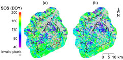
Figure 5 Spatial distributions of SOS (DOY) in 2001 (a) and 2003 (b).
Download figure:
Standard image High-resolution imageThe spatial SOS anomaly in pre-fire (2001) and post-fire (2003–2014) revealed the fire impacts on SOS (figure 6 and table 1). Before the fire occurrence, the anomaly was 0 for the areas of entire burn scar relative to the buffer zone although it varied from −1.0 to 3.0 d for different local areas. After the fire occurrence, the anomaly became highly variant, which showed considerably early SOS within the burn scar. The SOS anomaly during post-fire was strongly dependent on burn severity. It varied from −9.1 d in unburned/low severity to −18.5 d in high severity, and was −15.2 d for the entire burn scar. The difference of spatial SOS anomaly between pre-fire and post-fire was −8.1 d in unburned/low severity and −18.5 d in high severity. It was −15.2 d for the entire burn scar.
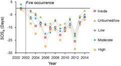
Figure 6 Interannual variation in the spatial SOS anomaly (SOSa) for different burn severity levels (Unburned/low, Low, Moderate, and High) and the entire burn scar (Inside).
Download figure:
Standard image High-resolution imageTable 1. The spatial SOS anomalies (unit: days) in pre-fire (2001) and post-fire (2003–2014) and their differences for different burn severity levels (Unburned/low, Low, Moderate, and High) and the entire burn scar (Inside).
| Burn severity | Unburned/low | Low | Moderate | High | Inside |
|---|---|---|---|---|---|
| Pre-fire | −1.0 | 0.0 | 3.0 | 0.0 | 0.0 |
| Post-fire | −9.1 | −10.7 | −14.3 | −18.5 | −15.2 |
| Difference | −8.1 | −10.7 | −17.3 | −18.5 | −15.2 |
Spatial SOS anomaly showed great variations interannually during the post-fire from 2003–2014 (figure 6). The magnitude (absolute value) of SOS anomaly increased from 2003–2006, remained relatively stable from 2006–2011, and decreased from 2011–2014. During the period of post-fire (12 years), the large anomaly occurred in 2006, 2009, and 2012, with a value of over 21 d for the entire burn scar and as large as 32 d in the high burn severity, which represented three troughs. In 2013 and 2014, the anomaly in the areas of unburned/low severity returned to the pre-fire status, which was −1.0 d in 2001 and −2.0 d in 2014.
3.3. Impacts of fire on SOS trend in 2001–2014
Figure 7 shows the comparison of the interannual variation in area-integrated SOS inside the burn scar and in the buffer zone during 2001–2014. Overall, SOS shifted early inside the burn scar relative to that in the buffer zone. The interannual variation in these two regions was similar in most years, particularly after 2009. However, the SOS trends during the study period were contrary for the buffer zone and burned area. It was 3.9 d/decade in the buffer zone, while it was −1.9 d/decade inside the burn scar. The dramatic SOS advance occurred in 2012, in which SOS was 35 d and 21 d earlier than that in neighboring years inside burn scar and in the buffer zone, respectively.
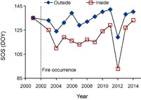
Figure 7 Interannual variation in area-integrated SOS inside the burn scar (Inside) and in the buffer zone (Outside) at the Hayman Fire area.
Download figure:
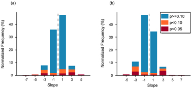
Standard image High-resolution imageThe SOS trend at the pixel scale was very complex. Figure 8 shows the pixel frequency with different trends inside the burn scar and in the buffer zone, respectively. In the buffer zone, SOS trend was positive in 55.4% of pixels (10.1% with p < 0.1) and it was negative in 44.6% of pixels (7.0% with p < 0.1). In contrast, the SOS trend inside the burn scar was positive in 41.4% of pixels (7.5% with p < 0.1) and it was negative in 58.6% of pixels (10.0% with p < 0.1).
Figure 8 The pixel frequency of SOS trend (days/year) in the buffer zone (a) and inside the burn scar (b) during 2001–2014.
Download figure:
Standard image High-resolution image
4. Discussion and conclusions
This study examined the wildfire impact on LSP SOS in the Hayman Fire. Evergreen forests were dominant across the regions before fire occurrence. However, the fire occurrence in 2002 disturbed land surface, which resulted in the conversion of forests to shrublands and grasslands according to the NLCD in 2001 and 2006 (figures 1 and 3). As a result, LSP SOS inside the burn scar advanced dramatically, which was 15.2 d on average, compared with the undisturbed buffer zone outside the burn scar (as a reference). The SOS advance was mainly associated with the fact that shrubs, grasses, and young trees usually unfold their leaves earlier than mature trees (Badeck et al 2004, Seiwa 1999). The LSP SOS was also strongly influenced by burn severity, which was quantified using the spatial SOS anomaly. In the areas with unburned/low burn severity, the vegetation disturbance was light, so that the SOS anomaly was generally less than 10 d during the post-fire (2003–2014). However, it could be as high as 32 d in the high burn severity. Note that the land cover conversion caused by wildfire could also change the local environment such as skin temperature because land surface energy balance varies among different vegetation types (Lee et al 2011, Shen et al 2015). The alteration of skin temperature could also have effects on vegetation phenology, which is worth investigating in the future but is beyond the scope of this study.
The interannual variation in EVI2 is likely to track well the gradual progresses of vegetation regeneration. The annual minimum EVI2, representing the greenness of evergreen trees (including evergreen forests and evergreen shrubs) during winter period when there were no green leaves on deciduous species, showed a relatively low and stable rate of recovery through 2003–2014. This trend agrees well with field observations indicating the slow progress of regeneration by tree seedlings after the Hayman Fire burning, particularly in the high severity burned areas (Chambers et al 2016, Rhoades et al 2011). On the other hand, the annual maximum EVI2, representing greenness from shrubs, grasses, and forests, showed two stages from 2003–2014. It recovered rapidly from 2003–2007, coinciding with the field observations that understory plant communities returned back to the cover of the pre-fire levels by 2007 (Fornwalt and Kaufmann 2014). The lower maximum EVI2 inside the burn scar relative to the references in the buffer was the result of low abundance of evergreen trees after the fire. After 2007, the increasing rate of the maximum EVI2 slowed down and became comparable to that of the minimum EVI2. This indicates that the interannual trend in both minimum and maximum EVI2 represented gradual regeneration of evergreen trees after the completion of understory recovery. Overall, the annual maximum and minimum EVI2 trajectories from 2003–2014 suggest that vegetation greenness could recover to pre-fire status in 2022 and 2053 at the current rates respectively. Of course, this projection is of high uncertainty because the influence of climate change and species interactions make the projection of forest recovery very complex (Miller et al 2013). However, the recovery was not reflected in NLCD land cover maps in 2006 and 2011. This is mainly due to the NLCD classification system that defines forests as the areas dominated by trees generally higher than 5 m tall while young trees lower than 5 m are classified as shrubland (Homer et al 2007). Tree growth is relatively slow in this area. For example, newly-established ponderosa pine in the Colorado Front Range takes more than 20 years to get 1–2 m tall (Huckaby et al 2003) and 20 year old Douglas-fir in the Northern Rocky Mountains is less than 2.4 m (Ferguson and Carlson 2010). Moreover, land cover type is classified based on the entire pixel, which is unlikely to detect the subpixel variation of tree recovery.
The forest recovery could further be connected to LSP SOS trajectories. The magnitudes of spatial SOS anomalies continuously increased during 2003–2007, corresponding to the increase of understory species coverage (Fornwalt and Kaufmann 2014). After 2007, the magnitudes of SOS anomalies showed decreasing trends, in response to the continuous regeneration of evergreen trees and relatively stable understory (Chambers et al 2016, Rhoades et al 2011). In particular, the magnitude of SOS anomalies became smaller after 2013, which is likely associated with the denser tree canopy causing less understory detected by satellites.
The magnitude and direction of the interannual trend of LSP SOS were also significantly altered by the Hayman Fire. The interannual trend was converted from 3.9 d/decade in the unburned buffer zone to −1.9 d/decade inside the burn scar during 2001–2014. It is likely that the fire impacts on LSP SOS will continue during the long recovery period. However, climate change may play a more and more important role in the interannual variation of SOS with the forest recovering.
The time series SOS further revealed that extreme weather and climate events had relatively less profound impacts on vegetation phenology than fire events did in a long-term period. In 2012, the contiguous United States experienced an exceptionally warm spring and the most severe drought since 1930s (Wolf et al 2016). The warmest spring greatly advanced the SOS across the region of the Hayman Fire, while the advanced days were much larger inside the burn scar than those in the buffer zone because of the difference in land cover types. On the other hand, severe droughts reduced the annual maximum EVI2 but had little impacts on the minimum EVI2 even in the following year. However, such dramatic impacts on vegetation phenology only appeared in the specific years (a short time period), and vegetation (including seasonal timing and magnitude) generally recovered quickly in the following few years.
The result from this study suggests that it should be cautious against simply viewing LSP trends as indicative of climate change. Although the interannual LSP detected from AVHRR and MODIS data has been widely associated with climate change in regional or global scales (de Beurs and Henebry 2005b, de Jong et al 2011, Zhou et al 2001, Zhang et al 2007), land disturbances caused by both natural processes (including insect outbreak, storm damage, flooding, drought, and wildfire) and human activities (including urbanization and deforestation) are likely to interrupt the trends reflecting climate change. This is due to the fact that disturbances can result in rapid conversions of the vegetated land surface, including profound changes in community composition as a result of biotic invasions, either through native range expansion, introduced species, or outbreaks of pathogens (Bradley et al 2010, Mack et al 2000). Even though the disturbance could be identified using the change detection approaches if it occurred several years away from either the start or end of a long-term phenological time series (de Beurs and Henebry 2005a, Verbesselt et al 2010), the detection would be very challenging in this study in which the disturbance happened only one year later than the begin of the time series. As a result, reliable phenological trends associated with climate change could be obtained if the pixels with land disturbances were explicitly subtracted.
Finally, it should be aware that the impact of land disturbance on LSP is likely to act more widely. It is due to the fact that fire frequency and size have increased and the trend will continue (Westerling et al 2006) and that human populations and their use of land have modified about one-third to one-half of the land surface and transformed another third or more of the terrestrial biosphere into rangelands and seminatural anthromes (Ellis 2011, Vitousek et al 1997). Thus, studies with longer temporal periods and larger spatial scales are still required to move forward.
Acknowledgments
This work was supported by NASA contracts NNX15AB96A and NNX14AQ18A. We obtained MTBS data from www.mtbs.gov, NLCD data from www.mrlc.gov, and MODIS products of MOD09GQ, MOD09GA, and MOD11A1 from https://lpdaac.usgs.gov/dataset_discovery/modis/modis_products_table.