
Abstract
Titanium alloys are known to have some excellent properties, such as good biocompatibility, good fatigue resistance and high strength to weight ratio. Due to these properties, Ti6Al4V alloy is widely used in the biomedical field, aerospace and automobile industries. In this article, pulse on-time (TON), pulse off time (TOFF), and servo voltage (SV) were selected as process parameters for wire electric discharge machining (WEDM) on Ti6Al4V alloy. The material removal rate (MRR) and surface roughness (SR) were determined as responses. MRR and SR have been equated by a central composite design (CCD: a response surface method technique). Then multi-objective Artificial Bee Colony optimization (MO-ABC) with Gray relational analysis (GRA) was selected as a priori approach for multi-objective optimization. Also, a multi-objective grasshopper optimization algorithm (MO-GOA) has been chosen as a posterior approach for optimization. These two algorithms have been tested on various iterations and populations. Based on the elapsed time, it has been found that the priori approach of multi-objective optimization is better than the posterior approach of multi-objective optimization. When comparing these algorithms based on the results, it is obtained that the posterior approach gives a better combination of multiple results. The major outcome of the research is that the priori method is quick, while the posterior approach produces many promising solutions.
Export citation and abstract BibTeX RIS

Original content from this work may be used under the terms of the Creative Commons Attribution 4.0 licence. Any further distribution of this work must maintain attribution to the author(s) and the title of the work, journal citation and DOI.
1. Introduction
Titanium is the ninth most abundant material found in the Earth's crust. Nevertheless, due to the complexity of its extraction process, it is one of the costly materials that limits its use [1]. Titanium undergoes an allotropic transformation at 882.50C, which changes its phase from alpha to beta. The addition of certain elements to titanium metal that raises its transition temperature are called alpha stabilizers. They are Al, O, N, and C. The elements that lower the transition temperature of titanium metal are called beta stabilizers, and they are Mo, V, Nb, Cu and Si. The elements with minimal effect on the transition temperature of titanium metal are called neutral elements, and they are Sn & Zr. In Ti6Al4V alloy, Al is added as alpha stabilizer, while V is added as beta stabilizer. The alpha phase of substances is a closed-packed hexagonal system of an elementary crystal structure type. The alpha phase of titanium is highly corrosion resistant, while the beta phase of substances is a body-centered cubic crystal structure type & the beta phase of titanium is more ductile. The Ti6Al4V alloy has an alpha + beta phase, where the best combination of both is applied. Therefore, Ti6Al4V is a good ductile, strong, formable, and corrosion-resistant alloy [2–11].
Titanium has a high strength-to-weight ratio, even at elevated temperatures. Due to this, titanium is widely used in the aerospace and automobile sectors [12]. Titanium is a highly corrosion resistant metal used in chemical industries [13]. When titanium is implanted in the human body, an oxide film forms on the titanium metal (due to its goodness), and it prevents corrosion and helps in osteointegration. Therefore, titanium has good biocompatibility and is therefore used in making biomedical implants [14, 15]. However, in addition to its good properties, titanium alloys have some difficulties in conventional machining due to other properties (such as high strength even at elevated temperatures, high chemical reaction propensity and low thermal conductivity) [16–19]. Therefore, for the machining of Ti6Al4V alloys, unconventional machining is one of the better choices [20]. In this study, WEDM is used as an unconventional machining for Ti6Al4V alloy. In WEDM, a wire is used to cut the workpiece by creating a spark between the wire and the workpiece [21–23]. This spark during machining depends on factors such as TON, Toff, SV, wire tension (WT), wire feed rate (WFR), etc TON, Toff, and SV are chosen as process parameters in this study.
Chopra et al investigated the power consumption on En31 steel during WEDM. They found that MRR and power consumption increase with increase in TON and decrease in voltage [24]. Ubale et al optimized WEDM on W-Cu metal matrix composites. They found a 24.11% improvement in MRR and a 27.45% improvement in SR due to the desirability task multi-objective optimization approach [25]. Siva Kumar et al processed titanium based human implant material via wire EDM. They found that good surface quality could be achieved due to WEDM [26]. Prabhu et al compared brass and molybdenum wire during wire-cut EDM using GRA with PCA. They found that molybdenum wire gives good surface quality. Whereas they found that maximum MRR and SR are achieved at high peak current [27]. Pranamik et al investigated the geometric error during WEDM on Ti alloy. They found that wire tension and flushing pressure are the most important factors for geometric error [28]. Singh et al studied the development of powder mix EDM and found that PMEDM can overcome the downside of EDM [29]. Jain and Parashar review the EDM process on Biomedical Materials. They have found that the EDM process makes the biomaterial more biocompatible [30].
Devarasiddappa et al performed WEDM on Ti6Al4V alloy. Four process parameters, TON, Toff, current (Ip), and wire-speed (WS), were chosen to analyze MRR and Sr Their research modeled the two responses and then selected a TLBO-based multi-objective optimization algorithm to simultaneously maximize MRR and minimize Sr [31].
Sharma et al Proposed WEDM on aero-engine alloy A-706. They have selected Toff, TON, SV, and WFR as input parameters. While MRR is maximized and SR is minimized. They found that WEDM cut surfaces have high amounts of molten droplets, craters, and microscopic holes due to improper flushing and high energy levels. They also concluded that good surface morphology and lowest roughness values are observed on TON 105 μS, SV 60 V, and Toff 55 μS due to low discharge energy and better flushing action [32].
Srinivasrao G et al performed WEDM on alpha-beta Ti alloy. They considered five input process parameters: TON, Toff, Ip, SV, and WFR. At the same time, MRR and SR were chosen as responses. They found that the optimized MRR 2.78066 mm3 min−1 and SR 1.292 micro-meters achieve on the TON 108 μS, Toff 51 μS, Ip 12 A, Vs 51 V, and WFR at 15 m min−1 [33].
Singh et al examined WEDM for the surface roughness of AISI H13 using the ANOVA method. They have found that the SR is minimum when using a diffused wire. SR is max for plain brass wire and high pulse on time [34].
Saini et al optimized the WEDM parameters considering the MRR and SR as the responses. They have found that MRR and SR increase while pulse on time increases [35].
Goyal et al performed WEDM on H-13 die tool steel considering TON, TOFF, wire type and peak current as process parameters. They concluded from ANOVA that TON is the most important factor influencing MRR and SR [36].
Babu et al proposed a feed-forward neural network model using adaptive particle swarm optimization algorithms to optimize surface roughness during drilling. They found that adaptive PSO gives results very close to experimental [37].
Karboga et al introduced ABC optimization for real-world problems, and they proved that it has better performance than other types of algorithms [38]. Mirjalili et al proposed a new algorithm for adaptation from locust swarm navigation in nature. This algorithm can provide competitive results in Pareto optimal solutions related to other algorithms [39]. Therefore, the priori type artificial Bee colony optimization algorithm and the posterior type grasshopper optimization algorithm were compared in this study.
The novelty of this work is to explore the machinability aspect of WEDM on Ti6Al4V alloy and optimize the responses by comparing the primary and posterior approach type algorithms. The research gap of this work is to consider responses other than MRR and SR in order to understand the full machinability aspect of WEDM. Different responses can be kerf width, recast layer thickness, micro-hardness, residual stress, maximum peak-to-valley height, etc.
2. Experimental process
In this investigation, a sample length of 240 mm and 4.8 mm thickness of the Ti6Al4V sample was taken as the machined length for WEDM. Each sample length has been machined at different process parameter conditions. In the present work the experiments were performed on the FANUC ROBOCUT ALPHA1iB wire cut electric discharge machine. It is shown in figure 1, and its manufacturer is FANUC Corporation Japan. In these experiments, a 0.25 mm hard brass wire has been selected as the wire material. At the same time, deionized water is used as the dielectric medium. The machine can bear a maximum workpiece weight of 1000kg and is 13KVA in power. This machine has an X-axis of 550 mm, a Y-axis of 370 mm, and a Z-axis of 310 mm.
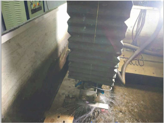
Figure 1. Wire cut electric discharge machine Setup.
Download figure:
Standard image High-resolution imageWEDM has a lot of process parameters. Some are the following:
- 1.Pulse ON Time: It is the time period in which current flows during machining.
- 2.Pulse OFF Time: This is the time period in which no current is supplied between the electrodes.
- 3.Servo Voltage: This is the voltage maintaining the spark gap between the electrode and the workpiece.
- 4.Wire Tension: Wire tension is a load in the wire. Which straightens the wire by continuously feeding the wire between the wire guides.
- 5.Peak Current: Peak current is the amount of current flowing in the wire to cut the workpiece by spark generation.
Machining process parameters such as TON, TOFF and SV significantly affect the quality of the products that manufactured by WEDM. Setting the right parameters can result in high MRR and low SR performance. These three parameters were selected on the basis of literature review and pilot experiment.
In this work, the surface roughness is measured by Surf Test SJ-210.During the measurement, the cut-off length was 0.8 mm, the sample length was 4.8 mm, and the measuring speed was 0.5 mm s−1. In this surface tester, a contact-type diamond probe is used as a sensor to measure surface roughness. In this experiment, the arithmetic mean height (Ra) indicates the mean absolute value along the sample length.

Here, ls is the sampling length, while Z (x) is the absolute roughness value from the mean.
Jewelry and medicine weighing scales were used to measure weight in this research. The Baijnath Premnath Atom MH 88 Palm Scale has an accuracy of 10 mg (0.01 g). Time was measured during the experiments with a stopwatch.

Here  is the initial weight,
  is the final weight after the experiment, and T is the Time during the experiment [40].
The central composite design was used to design the experiments. WEDM has a lot of input process parameters like a TON, Toff, SV, Ip, WS, WT, etc Nevertheless, according to some researchers, the most commonly affected process parameters are TON, Toff and SV that affect WEDM on Ti6Al4V. In table 1 Five levels of TON, five levels of Toff, and five levels of SV were selected according to the feasibility of the machine by the operator's experience and previous research.
Table 1. Levels of process parameters of WEDM.
| S.No. | Parameters | Units | Symbol | Range |
|---|---|---|---|---|
| 1 | Pulse ON Time | μS | TON | 6,8,10,12,14 |
| 2 | Pulse OFF Time | μS | TOFF | 20,22,25,27,30 |
| 3 | Servo Voltage | V | SV | 30,35,40,45,50 |
The CCD for the three factors has 2^3 (8) factorial runs, 2*3 (6) star runs, and six replicas of the centre levels, i.e., 20 experiments are done. The readings of the responses measured at these settings of the experiments are shown in table 2 below.
Table 2. Experimental chart for WEDM.
| Run | Pulse on time | Pulse off time | Servo voltage | MRR | SR |
|---|---|---|---|---|---|
| μS | μS | V | g/h | μm | |
| 1 | 12 | 22 | 45 | 3.102 | 4.803 |
| 2 | 12 | 27 | 45 | 3.342 | 4.901 |
| 3 | 10 | 25 | 40 | 2.664 | 4.401 |
| 4 | 12 | 22 | 35 | 3.048 | 4.855 |
| 5 | 12 | 27 | 35 | 3.276 | 4.998 |
| 6 | 10 | 25 | 30 | 2.166 | 5.141 |
| 7 | 10 | 20 | 40 | 2.238 | 4.601 |
| 8 | 6 | 25 | 40 | 2.526 | 2.801 |
| 9 | 10 | 25 | 40 | 2.910 | 4.398 |
| 10 | 10 | 25 | 40 | 2.616 | 4.451 |
| 11 | 10 | 25 | 40 | 2.568 | 3.981 |
| 12 | 8 | 22 | 35 | 2.286 | 3.952 |
| 13 | 10 | 30 | 40 | 3.144 | 4.612 |
| 14 | 10 | 25 | 40 | 2.964 | 3.950 |
| 15 | 10 | 25 | 50 | 2.286 | 4.957 |
| 16 | 8 | 27 | 35 | 2.706 | 3.654 |
| 17 | 8 | 22 | 45 | 1.902 | 3.801 |
| 18 | 8 | 27 | 45 | 2.604 | 3.481 |
| 19 | 14 | 25 | 40 | 3.810 | 5.201 |
| 20 | 10 | 25 | 40 | 2.988 | 4.105 |
3. Optimization
3.1. Multi-objective artificial bee colony optimization
Basically artificial bees in an artificial bee colony are classified into three categories:
- I.Employed bees.
- II.Onlooker bees.
- III.Scout bees.
Generally, bees visit the food source and collect nectar from them. This principle is used in MO-ABC to optimize the responses. The employed bees first search for the food source and then evaluate its nectar. The number of all employed bees and onlooker bees equals the number of food sources. While the amount of nectar is proportional to the fitness value, the state of the food source is the state of the solution. When all employed bees complete the evaluation of nectar, each employed bee goes randomly to a neighbouring food source by equation (3) and reevaluates the nectar.

Here, xi & xj are the ith & jth position of the bee, xi,j is the position of the new bee, & ϕ is the acceleration coefficient.
If this new position xij of the food source has more nectar than the previous one, update it to be the new position of the ith bee. After a food source assessment of these employed bees, onlooker bees come into play. When the nectar of a food source is better, the employed bees begin to dance, and on the dance area, the onlooker bees update the position of their food source by equation (4).

Here, xi is the ith position of the food source obtained by the Roulette Wheel Selection, & xj is the jth neighbouring food source position of the bee, xi,j is the position of the new bee, & ∅ is the acceleration coefficient. In roulette wheel selection, the probability of ith onlooker bee selection is pi obtained by equation (5):

Here, fitnessi is the fitness of ith bee, while n is the total no. of bees.
When all these employed and sighting bees move randomly near neighbouring food sources & the bees do not update for several cycles (if no better solution is found). So, the scout bees come into play, and this number of cycles is called the abandonment limit. The positions of the scout bees are updated randomly by a uniform distribution (equation (6)):

The best status of bees is updated. After that, the cycles continue and repeat. The iterations are stopped when the iteration reaches the maximum number of iterations defined in the initial step. Bees attain the best source of food and its best nectar [38].
In this article, the priori type multi-objective artificial bee colony algorithm was used to optimize MRR and SR simultaneously. The pseudocode and flow chart for the multi-objective ABC algorithm is shown in figures 2 and 3, respectively. For this, the weightage for each response was determined by the GRA method, the details of which are as follows:
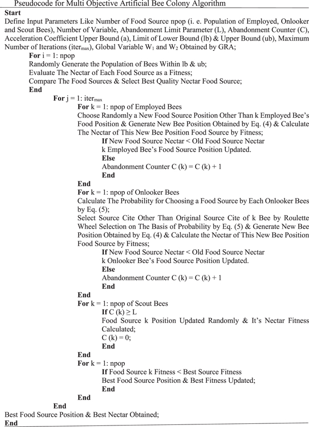
Figure 2. Pseudocode for Multi-Objective ABC.
Download figure:
Standard image High-resolution image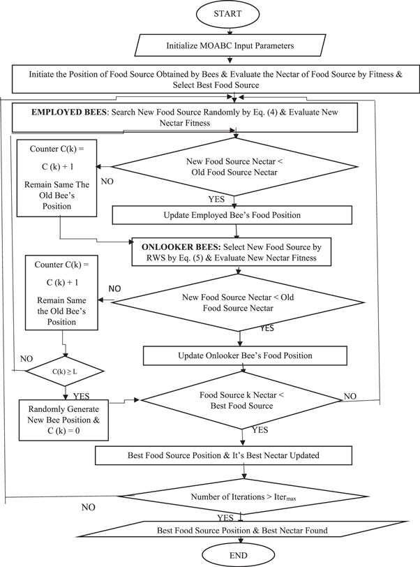
Figure 3. Flowchart of Multi-objective ABC.
Download figure:
Standard image High-resolution image3.1.1. Gray relational analysis
In the priori approach to multi-objective optimization, the equations for all responses are reduced to a single equation by assigning different weights to those responses. The advantage of GRA is that the weightage of the responses is determined by its experimental results. So, for this priori approach of MO-ABC, the problem can be formulated as:

Here, W1 and W2 are the weightings of MRR and SR, respectively. 1/MRR is taken to minimize the MRR (as we want to maximize the MRR). For this, MRRmax and SRmin are calculated as a single objective function taking W1 = 1, W2 = 0, and W1 = 0, W2 = 1, respectively. At the same time, MRR and SR are regression equations derived from DOE.
The GRA method can be understood through the following steps:
Step I
First, the responses are normalized by equation (8) (if one wants to maximize) and equation (9) (if one wants to minimize) [41]:


Here,
 is the normalized value of the nth number of the experimental run for oth response.
 is the experimental value of the nth number of the experimental run for oth response.
Step II
After normalizing the responses, the Gray Relational coefficient (GRC) is calculated by equation (10), & shown in the following table 3:

Table 3. Grey relational code.
| Pulse on time | Pulse off time | Servo voltage | MRR | SR | GRC MRR | GRC SR |
|---|---|---|---|---|---|---|
| μS | μS | V | g h−1 | μm | ||
| 8 | 22 | 35 | 2.286 | 3.952 | 0.384988 | 0.510421 |
| 12 | 22 | 35 | 3.048 | 4.855 | 0.555944 | 0.368777 |
| 8 | 27 | 35 | 2.706 | 3.654 | 0.463557 | 0.58451 |
| 12 | 27 | 35 | 3.276 | 4.998 | 0.641129 | 0.353253 |
| 8 | 22 | 45 | 1.902 | 3.801 | 0.333333 | 0.545455 |
| 12 | 22 | 45 | 3.102 | 4.803 | 0.574007 | 0.374766 |
| 8 | 27 | 45 | 2.604 | 3.481 | 0.441667 | 0.638298 |
| 12 | 27 | 45 | 3.342 | 4.901 | 0.670886 | 0.363636 |
| 6 | 25 | 40 | 2.526 | 2.801 | 0.426273 | 1 |
| 14 | 25 | 40 | 3.810 | 5.201 | 1 | 0.333333 |
| 10 | 20 | 40 | 2.238 | 4.601 | 0.377672 | 0.4 |
| 10 | 30 | 40 | 3.144 | 4.612 | 0.588889 | 0.398539 |
| 10 | 25 | 30 | 2.166 | 5.141 | 0.367206 | 0.338983 |
| 10 | 25 | 50 | 2.286 | 4.957 | 0.384988 | 0.357569 |
| 10 | 25 | 40 | 2.568 | 3.981 | 0.434426 | 0.504202 |
| 10 | 25 | 40 | 2.964 | 3.95 | 0.53 | 0.510856 |
| 10 | 25 | 40 | 2.664 | 4.401 | 0.454286 | 0.428571 |
| 10 | 25 | 40 | 2.910 | 4.398 | 0.514563 | 0.429031 |
| 10 | 25 | 40 | 2.616 | 4.451 | 0.444134 | 0.421053 |
| 10 | 25 | 40 | 2.988 | 4.105 | 0.537162 | 0.479233 |
Here,
 (r) = reference coefficient that is 1.

∆max = maximum value of 
∆min = minimum value of 
ξ = discrimination coefficient (0.5)
0 < ξ < 1, [42].
Step III
After the GRC is calculated, its average is calculated at each process parameter level. Then its maximum Range is calculated by equation (11), and the weight of each response is calculated by equation (12), as shown in table 4:


Table 4. GRA weightage for MRR & SR
| MRR (g h−1) | SR (μm) | ||||||
|---|---|---|---|---|---|---|---|
| Level | TON (μs) | TOFF (μs) | SV (V) | Level | TON (μs) | TOFF (μs) | SV(V) |
| −1.682 | 0.426 | 0.377 | 0.367 | −1.682 | 1 | 0.4 | 0.338 |
| −1 | 0.405 | 0.462 | 0.511 | −1 | 0.569 | 0.449 | 0.454 |
| 0 | 0.463 | 0.509 | 0.530 | 0 | 0.426 | 0.480 | 0.490 |
| 1 | 0.610 | 0.554 | 0.504 | 1 | 0.365 | 0.484 | 0.480 |
| 1.682 | 1 | 0.588 | 0.384 | 1.682 | 0.333 | 0.398 | 0.357 |
| R | 0.594 | 0.211 | 0.163 | R | 0.666 | 0.086 | 0.151 |
| ∑R | 0.968 | ∑R | 0.904 | ||||
| Weight | 0.517 | Weight | 0.483 | ||||
Here,
 = Range of grey relational coefficient.
A = Average grey relational coefficient of each process parameter at the same level.
o = 1, 2...... q is number of objectives.
t = 1,2,3......u is number of cutting parameters.
v = 1,2,3......w is number of levels of cutting parameters [43].
The weightage derived from GRA for MRR and SR is 0.517 and 0.483, respectively.
3.2. Multi-objective grasshopper optimization algorithm
Basically, in the Grasshopper Optimization Algorithm, the position of the grasshopper in the swarm represents a possible solution to the optimization. The position of the nth grasshopper can be represented as Zm and can be defined according to equation (13):

Here, Sn is the social interaction, Gn is the gravity force on the nth grasshopper, An is the wind advection.
Here in this article, the posterior approach type GOA is used to optimize the MRR and Sr First, the archive size, maximum number of iterations, population size, coverage parameters, attraction intensity (F), and attractive length scale (L) are defined. Then first, the position of the grasshopper is determined at random by the uniform distribution. Then its fitness is calculated. Then update the archive. If the non-dominated solution collection exceeds the maximum size, rank it, and truncate it to store the full extent. Then select any other mth grasshopper by roulette wheel selection. Then calculate the distance between random grasshoppers. Their social interaction is updated by equation (14).

Here, dmn is the distance between mth and nth grasshopper.

f is attraction intensity, L is attractive length scale.
Then the position of the grasshopper is updated by equation (16).

Here, C is the coverage parameter that shows the forces of attraction and repulsion between the grasshoppers. So, it is updated by equation (17).

Here, iter is the current iteration,  is the maximum number of iterations,
  is the maximum coverage,
  is the minimum coverage.
Then after this collection of locust positions its fitness is calculated, and the process is repeated again and again until the stopping criterion is reached. Then the final solution is obtained [39]. The pseudocode and flow chart for the multi-objective GOA algorithm is shown in figures 4 and 5, respectively.
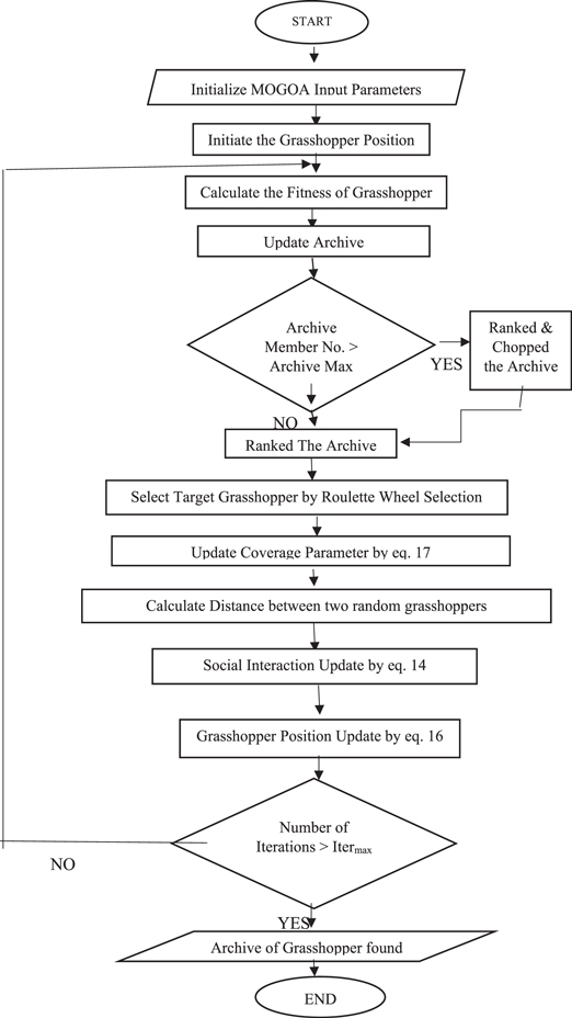
Figure 4. Flowchart of Multi-objective GOA.
Download figure:
Standard image High-resolution image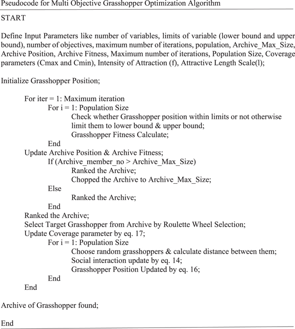
Figure 5. Pseudocode for Multi-Objective GOA.
Download figure:
Standard image High-resolution image4. Results and discussions
4.1. DOE analysis of MRR
For the material removal rate, the model's fitness is determined by the R2 value, which is 0.9318 and is very close to 1. It, therefore, reflects the excellent fitness of the quadratic model for MRR. At the same time, the difference between Adjusted R2 (0.8705) and Predicted-R2 (0.7374) is less than 0.2 and very close. So, it reveals the excellent quality of prediction of the quadratic model of MRR. Statistical Analysis of MRR is shown in table 5.
Table 5. Statistical Analysis of MRR.
| Parameters | Value | Parameters | Value |
|---|---|---|---|
| Std. Dev. | 0.1678 | R2 | 0.9318 |
| Mean | 2.76 | Adjusted R2 | 0.8705 |
| C.V. % | 6.09 | Predicted R2 | 0.7374 |
| Adeq Precision | 16.9878 |
In the analysis of variance for MRR, the model F-value is 15.19, and the corresponding p-value is < 0.0001, whereas for the lack of fit, the F-value is 0.5714, and the corresponding P-value is 0.7230, indicating good fitness of the quadratic model. The ANOVA suggests that the linear effect of TON and Toff, and the quadratic effect of TON and SV, significantly increase MRR. Whereas ANOVA for MRR is shown in table 6.
Table 6. ANOVA for MRR.
| Source | Sum of squares | df | Mean square | F-value | p-value | |
|---|---|---|---|---|---|---|
| Model | 3.848 | 9 | 0.4276 | 15.19 | 0.0001 | significant |
| A-Pulse On time | 1.988 | 1 | 1.988 | 70.64 | < 0.0001 | |
| B-Pulse off time | 0.655 | 1 | 0.655 | 23.28 | 0.0007 | |
| C-Servo voltage | 0.00019 | 1 | 0.00019 | 0.0069 | 0.9352 | |
| AB | 0.0642 | 1 | 0.0642 | 2.28 | 0.1617 | |
| AC | 0.0459 | 1 | 0.0459 | 1.63 | 0.2305 | |
| BC | 0.0154 | 1 | 0.0154 | 0.5473 | 0.4764 | |
| A2 | 0.2823 | 1 | 0.2823 | 10.03 | 0.0100 | |
| B2 | 0.0035 | 1 | 0.0035 | 0.1253 | 0.7307 | |
| C2 | 0.4223 | 1 | 0.4223 | 15.00 | 0.0031 | |
| Residual | 0.2815 | 10 | 0.0281 | |||
| Lack of fit | 0.1023 | 5 | 0.0204 | 0.5714 | 0.7230 | not significant |
| Pure error | 0.1791 | 5 | 0.0358 | |||
| Cor total | 4.130 | 19 |
The perturbation Plot for MRR is shown in figure 6. The perturbation plot shows that the MRR increases significantly due to higher discharge energy with an increasing TON. Whereas the Toff shows a slight increase in MRR because when the Toff increases, the flushing time increases, and more material is removed [31].
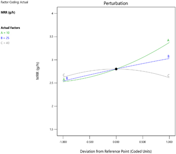
Figure 6. Perturbation Plot for MRR.
Download figure:
Standard image High-resolution imageIncreasing the SV increases the MRR, and further increasing the SV decreases the MRR. So, machining can be done very quickly (no wire breaks) at some optimum value of SV and increases the MRR due to good discharge energy [33].
The 3D plot for a TON versus Toff versus MRR shows that increasing TON and Toff together increases MRR. The 3D surface plot for MRR is shown in figure 7.
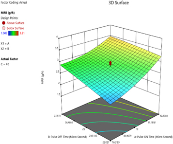
Figure 7. 3D surface plot for MRR.
Download figure:
Standard image High-resolution imageThe regression equation for MRR is shown in equation (18).
4.2. DOE analysis of SR
The R2 for SR is 0.9490, and the difference between adjusted R2 and estimated R2 is very close, i.e., it shows the excellent model prediction for Sr Statistical Analysis of SR is shown in table 7.
Table 7. Statistical analysis of Sr
| Parameter | Value | Parameter | Value |
|---|---|---|---|
| Std. Dev. | 0.1956 | R2 | 0.9490 |
| Mean | 4.35 | Adjusted R2 | 0.9031 |
| C.V. % | 4.49 | Predicted R2 | 0.8169 |
| Adeq Precision | 17.4231 |
For SR, analysis of variance shows that the quadratic model with an F value of 20.68 and a P-value <0.0001 shows good fitness. At the same time, the p-value and f-value for lack of fit for SR are 0.7885 (>0.05) and 0.4664 (very small), respectively. It, therefore, indicates the excellent fitness of the regression model for SR ANOVA suggests that TON is the most critical parameter that affects Sr ANOVA for SR as shown in table 8.
Table 8. ANOVA for Sr
| Source | Sum of squares | df | Mean square | F-value | p-value | |
|---|---|---|---|---|---|---|
| Model | 7.12 | 9 | 0.7912 | 20.68 | <0.0001 | significant |
| A-Pulse ON Time | 5.70 | 1 | 5.70 | 148.86 | <0.0001 | |
| B-Pulse OFF Time | 0.0002 | 1 | 0.0002 | 0.0054 | 0.9426 | |
| C-Servo Voltage | 0.0445 | 1 | 0.0445 | 1.16 | 0.3062 | |
| AB | 0.0932 | 1 | 0.0932 | 2.44 | 0.1497 | |
| AC | 0.0038 | 1 | 0.0038 | 0.1000 | 0.7583 | |
| BC | 0.0004 | 1 | 0.0004 | 0.0102 | 0.9215 | |
| A2 | 0.1166 | 1 | 0.1166 | 3.05 | 0.1114 | |
| B2 | 0.1823 | 1 | 0.1823 | 4.76 | 0.0540 | |
| C2 | 0.9460 | 1 | 0.9460 | 24.72 | 0.0006 | |
| Residual | 0.3827 | 10 | 0.0383 | |||
| Lack of Fit | 0.1218 | 5 | 0.0244 | 0.4669 | 0.7885 | not significant |
| Pure Error | 0.2609 | 5 | 0.0522 | |||
| Cor Total | 7.50 | 19 |
The perturbation plot also reveals the same results as ANOVA for Sr As the TON increases, the SR increases, Due to more discharge energy, more area is affected; hence the SR deteriorates. At the same time, Toff and SV have little effect on SR [33]. The SR decreases as the Toff increases due to the longer flushing time. When the pulse-off time increases rapidly, the SR increases slightly due to the accumulation of debris without flushing[31]. Similar results shown by the 3D plot for Sr Perturbation Plot for SR is shown in figure 8. The 3D surface plot for SR is shown in figure 9.
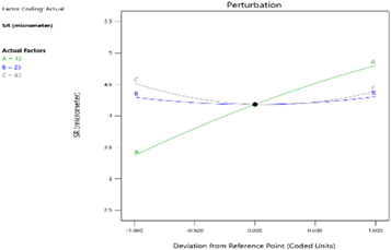
Figure 8. Perturbation plot for Sr.
Download figure:
Standard image High-resolution image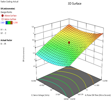
Figure 9. 3D surface plot for SR.
Download figure:
Standard image High-resolution imageThe regression equation for SR is shown in equation (19).
4.3. Optimization results
The priori approach type MOABC setting parameters are below. First, for this priori approach, 100% weight was given to each response and the individual optimum of MRR and SR was obtained. Whereas this was followed by multi-objective optimization giving 51.7% wt for MRR and 48.3% wt for SR, which was calculated by GRA. Here, three parameters have been selected for the experiments. Whereas on a combination of different populations and iterations, optimization is done.MO-ABC setting parameters are shown in table 9.
Table 9. Multi-objective ABC setting parameters.
| ABC Setting Parameters | Value |
|---|---|
| Number of Variable | 3 |
| Population Size | 200 & 50 |
| Maximum Iterations | 1000 & 500 |
| Acceleration Coefficient (a) | 1 |
| Global Variable (w1 & w2) | 0.517 & 0.483 |
The convergence curve is a curve that indicates how quickly the algorithm converges to the optimal value with a few iterations. The convergence curves for single objective MRR and SR are shown below in figure 10:
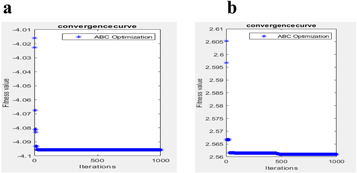
Figure 10. Convergence curve of ABC for (a) MRR (b) SR.
Download figure:
Standard image High-resolution imageFor different populations and iterations, MRR and SR are chosen as responses to analyze multi-objective ABC as priori approaches & shown in the following table 10 and figure 11. ABC shows that the maximum MRR is 4.0956 g h−1 @ TON 14 μs, Toff 30 μs, and SV 44.728 V. At the same time, the elapsed time is 2.939815 seconds for 500 iterations and 50 populations.
Table 10. Priori approach analysis for MOABC.
| S. No. | No. of iterations | No. of populations | Elapsed time | Optimized parameters | Optimized responses |
|---|---|---|---|---|---|
| Global Variable w1 = 1 w2 = 0, ABC for MRR | |||||
| 1. | 1000 | 200 | 11.534444 seconds | 14 μS, 30 μS, 44.7218 V | MRR 4.0956 g h−1. |
| 2. | 1000 | 50 | 5.114449 seconds | 14 μS, 30 μS,44.7310 V | MRR 4.0956 g h−1 |
| 3. | 500 | 50 | 2.939415 seconds | 14 μS, 30 μS, 44.7288 V | MRR 4.0956 g h−1 |
| Global Variable w1 = 0 w2 = 1, ABC for SR | |||||
| 4. | 1000 | 200 | 11.625708 Seconds | 6 μS, 28.1303 μS, 41.3728 V | SR 2.560 μm |
| 5. | 1000 | 50 | 5.298843 Seconds | 6 μS, 28.1275 μS, 41.5762 V | SR 2.561 μm |
| 6. | 500 | 50 | 3.163739 Seconds | 6 μS, 28.2819 μS, 41.2199 V | SR 2.561 μm |
| Global Variable w1 = 0.517 w2 = 0.483, MOABC for MRR | |||||
| 7. | 1000 | 200 | 11.507053 Seconds | 6 μS, 30 μS, 40.3709 V | MRR 2.67 g h−1,SR 2.615 μm |
| 8. | 1000 | 50 | 4.955235 Seconds | 6 μS, 30 μS, 40.3714 V | MRR 2.67 g h−1,SR 2.615 μm |
| 9. | 500 | 50 | 3.080010 Seconds | 6 μS, 30 μS, 40.3620 V | MRR 2.6724 g h−1,SR 2.615 μm |
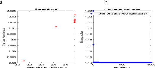
Figure 11. (a) Pareto front, (b) Convergence Curve. for Multi-objective ABC optimization.
Download figure:
Standard image High-resolution imageABC shows that the minimum SR is 2.561 μm @ TON 6 μs, Toff 28.2819 μs, and SV 41.2193 V. At the same time, the elapsed time is 3.163739 seconds for 500 iterations and 50 populations.
MOABC shows that the optimum SR is 2.615 micro-meter & optimum MRR is 2.67 g h−1, @ TON 6 μs, Toff 30 μs, and SV 40.3620 V. At the same time, the elapsed time is 3.080010 seconds, for 500 iterations and 50 populations.
Priori approach ABC shows that the elapsed time increases as the number of calculations increases.
A Pareto-front diagram is a diagram that shows how two responses affect each other. The Pareto-front diagram shows that maximum MRR is achieved at high Sr Priori approach type ABC also confirms the DOE results, that the MRR is higher on high TON, high Toff, and medium voltage. In contrast, the SR is minimal at the low TON, moderate Toff, and SV. When MRR and SR are formulated as a single priority problem in MOABC, optimum MRR and SR are obtained at a low TON, Toff, and moderate SV.
Whereas the posterior approach type MOGOA gives the combination of results in an archive to optimize MRR and SR together.
When we compare these two (priori-based MOABC and posterior type MOGOA) algorithms, it is found that a posteriori approach is better than the priori approach type algorithm as it gives a more optimal set of solutions. In contrast, the priori approach type algorithm only provides a single optimal solution. At the same time, the posterior approach algorithm took more elapsed time than the priority approach algorithm [44, 45].
The setting parameters, Pareto front, for the posterior approach MOGOA, are shown below in table 11, and figure 12, respectively:
Table 11. MOGOA setting parameters.
| MOGOA setting parameters | Value |
|---|---|
| Number of variables | 3 |
| number of objectives | 2 |
| Archive_Max_Size | 100 |
| Coverage parameters (Cmax and Cmin) | 1 to 0.00004 |
| Intensity of attraction (f) | 0.5 |
| Attractive length scale(l) | 1.5 |
| Population size | 200 |
| Maximum iterations | 1000 & 250 & 125 |
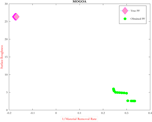
Figure 12. Pareto front for MOGOA.
Download figure:
Standard image High-resolution image
Posterior approach MOGOA gives several results. The optimum SR is 2.564 micro-meter & the optimum MRR is 3.0654 g h−1, @ TON 6 μs, Toff 28.6607 μs, and SV 41.2163 V. At the same time, another optimum result is MRR 4.0914 g h−1 & SR 5.931 μm @ TON 13.997 μs, Toff 29.6363 μs, and SV 44.2687 V. While the elapsed time is 42.990352 seconds for 200 iterations and 125 populations. The other results are shown in table 12.
Table 12. Posteriori approach analysis for MOGOA.
| Archive Solutions No. | Optimized Parameters | Optimized Responses |
|---|---|---|
| Population 200, Iteration 1000, Elapsed Time 343.129155 Seconds | ||
| 01. | 6 μs, 29.2895 μs, 40.8245 V | MRR 3.165 g h−1, SR 2.580 μm |
| 02. | 14 μs, 29.1108 μs, 44.0561 V | MRR 4.0857 g h−1, SR 5.812 μm |
| 03. | 12.4769 μs, 24.4981 μs, 40.8843 V | MRR 3.432 g h−1, SR 4.803 μm |
| Population 200, Iteration 250, Elapsed Time 87.689611 Seconds | ||
| 04. | 14 μs, 22.3893 μs, 41.2890 V | MRR 3.9474 g h−1, SR 4.993 μm |
| 05. | 6 μs, 30 μs, 39.3913 V | MRR 3.2826 g h−1, SR 2.6391 μm |
| 06. | 6 μs, 28.1858 μs, 41.2342 V | MRR 2.9964 g h−1, SR 2.561 μm |
| Population 200, Iteration 125, Elapsed Time 42.990352 Seconds | ||
| 07. | 6.0001 μs, 28.6607 μs, 41.2163 V | MRR 3.0654 g h−1, SR 2.564 μm |
| 08. | 13.9997 μs, 29.6363 μs, 44.2687 V | MRR 4.0914 g h−1., SR 5.931 μm |
| 09. | 6 μs, 29.9932 μs, 39.7702 V | MRR 3.4692 g h−1, SR 4.825 μm |
In figure 12, the true Pareto-front is compared with the obtained Pareto-front. This indicates that the obtained Pareto-front is in a viable range. The MOGOA Pareto Front also shows that higher MRR achieves at higher Sr.
5. Conclusion
The present research work is undertaken to correctly understand the difference between the primary approach of multi-purpose optimization and the posterior approach of multi-purpose optimization while performing WEDM on Ti6Al4V alloy. Mathematical modelling of MRR and SR is done using CCD. The ANOVA shows the critical factors influencing MRR and Sr Whereas the 3D plot and perturbation plot show the effect of process parameters on MRR and Sr Then fits the regression model for MRR and Sr GRA is applied for weightage calculation for MRR and SR, and then MO-ABC is applied. The posterior type MOGOA is then implemented to optimize the responses. Although the priori approach type ABC with a different number of counts gives similar results and these results are different for the posterior type MOGOA for the same number of counts. As the No Free Lunch Theorem shows, one algorithm is better for one class of problems, while for another problem, the other algorithm is promising. So, in this paper, both types of approaches are compared for a class of problems and find that the priori method is quick while the posterior approach gives many promising solutions. MRR is maximized for manufacturing purposes, whereas SR is minimized for good quality. The following points are also concluded here:
- 1.The CCD shows that the quadratic model is fitted for MRR and SR, respectively.
- 2.ANOVA for MRR shows, that the linear effect of TON, Toff, and the quadratic effects of SV & TON, are the most critical factors affecting MRR.
- 3.The MRR increases with an increasing TON and Toff.
- 4.According to ANOVA, the linear effect of TON and the quadratic effect of SV is the most critical factor for Sr.
- 5.Increasing the TON increases the Sr Other parameters like Toff and SV have little effect on Sr.
Data availability statement
All data that support the findings of this study are included within the article (and any supplementary files).