

Abstract
Reconfigurable freeform optical systems greatly enhance imaging performance within non-symmetric, compact, and ergonomic form factors. In this paper, several advances improve design, testing, and monitoring of these systems. Specific enhancements include definition of polynomials for fast and efficient parameterizations of vector distributions in non-circular apertures and merit based function optimization. Deflectometry system improvements enable metrology for almost any conceivable optic shape and guide deterministic optical figuring process during the coarse grinding phase by including modulated infrared sources. As a demonstration of these improvements, parametric optimization is tested with the tomographic ionized-carbon mapping experiment, a reconfigurable optical system. Other case studies and demonstrations include metrology of a fast, f/1.26 convex optic, an Alvarez lens, and real-time monitoring of an array of independently-steerable hexagonal mirror segments as well as an induction formed surface and inflatable Mylar mirror.
Export citation and abstract BibTeX RIS

Original content from this work may be used under the terms of the Creative Commons Attribution 4.0 license. Any further distribution of this work must maintain attribution to the author(s) and the title of the work, journal citation and DOI.
1. Motivation
Increasingly sophisticated optics are deployed in diverse fields such as astronomy, commercial photography, industrial manufacturing, and medical imaging. Evolving beyond the realm of traditional spherical surfaces, today's optics frequently employ aspheric optical surfaces, which have a departure from the best-fit sphere, or even more generic freeform optical surfaces, often defined by their lack of symmetry or non-predefined low order shape polynomials in contrast to off-axis conic surfaces (e.g. off-axis parabola).
Custom optics serve many purposes. Prior to mass production, a custom optic may be fabricated for prototyping. Next-generation telescopes [1–3] utilize custom mirrors manufactured and tested to their extreme precision specifications. Some optical systems contain deformable or moving elements which dynamically change the optical prescription. The one aspect underpinning all these examples is the need for flexibility. Custom optics fabrication is a growing industry that demands flexibility in all stages from design to testing since traditional metrology solutions are often lacking the dynamic range (e.g. nulling requirement for Fizeau interferometry) to accommodate verity of optical units under test or the spatial resolution (e.g. point cloud measurement using laser tracker) to guide the computer-controlled surface figuring processes.
Advancing that flexibility is the aim of this paper through discussion of reconfigurable optical systems. For this paper, a reconfigurable optical system is defined as a system whose optical properties can be quickly altered, either to accommodate substantially different optical elements (e.g. metrology system measuring both ground and polished surface) or to substantially alter the optical properties of a system (e.g. optical design with active elements changing the optical path). They are intended as systems that can be changed faster than design and fabrication of new hardware and with greater dynamic range than adaptive optics systems or interferometry which only perturb the optical design.
Optical design of reconfigurable systems (section 2) requires special considerations and mathematical tools. Reconfigurable optical metrology systems (section 3) allow precise measurement for a wide range of optical prescriptions. Systems which are actively configurable require dynamically updating measurements for feedback (section 4). All these items are discussed in this paper and demonstrated with practical optical examples.
This work is partly described in a previous conference publication [4] and provides substantial updates and additional materials summarizing the new technology developments conducted at the University of Arizona.
2. Optical design of reconfigurable systems
2.1. Math tools for characterizing surface and vector distributions
During the iterative sequence of design, fabrication and metrology, mathematical tools are required for describing surfaces and vector fields, such as distortion. Modal processing is one useful method for reducing a surface or vector distribution into a list of fit coefficients which can be accurately modeled by a computer [5–8]. Ideally the basis functions that make up these modal distributions are orthogonal, computationally robust, and efficient. Efficiency is critical for reconfigurable optical systems because the optical prescription is expected to substantially change and fast calculations permit rapid response. For dynamic metrology (example, section 4.1), numerical calculation speed may be the limiting factor in system performance.
One approach that meets these goals is employing a two-dimensional (2D) extension of Chebyshev polynomials to describe surfaces. Chebyshev polynomials have broad use in the optical community for applications ranging from phase unwrapping algorithms [9] to Gaussian beam diffraction [10].
Vector distributions are described by Chebyshev gradient polynomials [11], which can describe slope data, and Chebyshev curl polynomials [12] that describe rotational data. Both of these sets are orthonormal across rectangular apertures. If the common Laplacian terms are only included once, these gradient and curl polynomials can be used to fit any vector data in the rectangular domain.
Mathematically, the one-dimensional Chebyshev polynomials of the first kind (T) are defined as:

Two-dimensional Chebyshev polynomials (F) are expressed as:

Finally, the gradient and curl polynomials (G and C polynomials) [11, 12] are defined by the equations:


In general, the polynomial sets are defined in the Cartesian coordinate system, with (x, y) axes. Terms m and n are indices of polynomial functions in x and y, respectively. They are both positive integer values in the range 0 to infinity. They are used to denote the order of the polynomial. For 2D polynomials, an additional variable, j, is introduced that denotes the order of the polynomial, in the same way that m and n denote polynomial order for 1D polynomials. Since the 2D polynomials are a function of 1D polynomials, j can be written in terms of m and n and this relation is described in [11]. The terms  and
and  represent unit vectors in the x and y directions, respectively. The terms with the prime symbol (') denote gradients, e.g. T' (x) is the gradient of T in the x dimension.
As an example of the vector polynomials, consider modeling imaging distortion with a quiver plot from a three mirror anastigmat system with rectangular aperture as shown in figure 1 [12]. The model is taken from the standard Zemax OpticStudio [13] library.
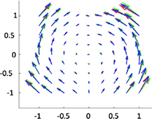
Figure 1. Quiver plots from a simulated camera's distortion fitting. Red arrows are the ideal (simulated) values, green arrows are results from S and T fitting, and blue arrows are the results from G and C fitting. The quiver plot is downsampled and arrows are magnified 1.5×. Figure credit: [12].
Download figure:
Standard image High-resolution imageThe distortion map is fit once with the G and C polynomials and then for comparison, it is fit another time using Zernike-based S and T polynomials [14, 15]. For both sets of fittings, the first 12 (6 gradient and 6 curl) polynomials were chosen. However, the common terms in both sets (i.e. for which the Laplacian is zero) was only counted once.
To show the performance of the Chebyshev-based vector polynomial, residual error from both polynomial fits was calculated as the RMS (root mean squared) error in x and y position as well as percentage errors in both positions, calculated as follows:
% Error = 100% × [rms (real error)/RMS (reference position)] (6) .
Here, the reference position means the ideal (simulated) distortion, i.e. predicted—real position from the distortion map.
As can be seen from table 1, the G & C polynomial based fitting provides a more accurate representation of the ideal distortion map, with lower error in both x and y positions.
Table 1. Fitting performance comparison of the two vector polynomial set cases to represent/model the simulated camera's distortion map.
| S and T polynomial fit | G and C polynomial fit | |||
|---|---|---|---|---|
| x-position | y-position | x-position | y-position | |
| Real error (µm) | 0.593 | 0.654 | 0.255 | 0.285 |
| % Error (%) | 12.44 | 8.30 | 5.35 | 3.62 |
These Chebyshev-based polynomials maintain several advantages [11, 12] over other sets of polynomials. To start, the vector sets can be derived straightforwardly from the scalar sets without needing any orthogonalization techniques, such as Gram–Schmidt orthogonalization. Additionally, Chebyshev polynomials have well-known recursion relations that can be computed very quickly and with minimal loss of numerical precision. For the design and analysis of reconfigurable optical systems, these polynomials offer significant advantages.
2.2. Fitness function-based optical system design
For some reconfigurable optical systems utilizing multiple beam paths sharing a common optical component (e.g. Dynamic K-mirror system in section 2.3) freeform optics are often used in order to correct configuration-dependent wavefront aberrations. Traditional optical design approaches require human's intuition in order to select the optimal location and numbers of the freeform optics, which significantly impact the overall manufacturing cost and alignment tolerancing. The modal mathematical framework (section 2.1) combined with an objective freeform surface selection process provides an efficient optical system design and optimization capability.
When evaluating a design to determine if breaking rotational symmetry and employing freeform surfaces [16] is worth the effort, a data-driven methodology should be employed. The decision to increase the number of degrees of freedom through freeform surfaces can yield reduced volume, increased field of view, or increased imaging performance [17, 18], but typically comes at a high cost. Therefore, careful choice of which surfaces to apply freeform terms is necessary in order to maximize their impact.
To guide this selection process, a parametric fitness function is developed using modal wavefront fitting [19, 20]. The fitness function combines multiple metrics from aberration control to manufacturability to provide a single data-driven metric. The detailed prescription of the fitness function and its actual optical design application is available [19, 20].
Equation (5) is one form of the fitness function proposed,

where  is the minimum fractional overlap between the forward
  and the reverse
  data, which captures the input data quality.
  and
and  are parameters capturing how well a single surface represents the ensemble of all input data at the surface.
  and
and  are parameters that capture the amount of potential aberration correction over the entire field of view at the surface.
  is the parameter to represent the difficulty manufacturing the surface. Each parameter set has its own unique weight and sums together to provide a single metric to evaluate the surface, where a large positive value of the function is optimal.
The data used to inform the selection comes from forward and reverse ray trace data at every surface of interest within the design. An aberrated optical system will have discrepancies between these data, while a non-aberrated system will have identical data, as shown in figure 2.
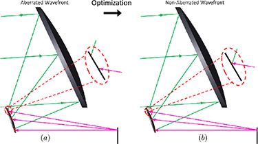
Figure 2. Forward (green) and reverse (magenta) ray data is used as the input to the parametric fitness function. As optimization converges to a local minimum, the aberrations in the system are reduced and the two data sets converge as shown in the call-out. Figure credit: [4].
Download figure:
Standard image High-resolution imageThe typical goal of optimization is to take an aberrated system and turn it into a non-aberrated system. Therefore, throughout the process of optimization, as more freeform terms are employed, the data input into the fitness function will converge.
2.3. Dynamic K-mirror optical system design
To validate efficiency of the computational tools, the parametric fitness function is employed on a real-world project, the tomographic ionized-carbon mapping experiment (TIME) [21, 22] including a reconfigurable dynamic K-mirror configuration. The dynamic system is needed to de-rotate the field on the sky.
Shown in figure 3 is an optical design optimized in Zemax that utilized freeform surfaces on K2, P1, P2, and C1. This system enables a linear field of view mm-wave experiment on the 12 m Atacama large millimeter array (ALMA) [23] prototype radio telescope.
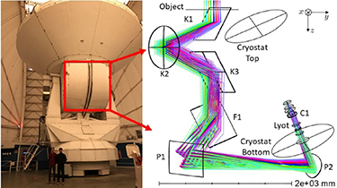
Figure 3. The 12 m ALMA prototype radio telescope (left) on Kitt Peak in Arizona with its cabin called out, which houses the TIME (right). The TIME optical design required an extremely folded beam path to fit the large linear field of view and cryostat in the defined volume of the telescope cabin. Figure credit: [4].
Download figure:
Standard image High-resolution imageThe mirrors for TIME and their mechanical structure have been fabricated out of aluminum, as shown in figure 4. The mechanical position of the mirrors and sled was set by a laser-tracker, first in a laboratory setting (a) and (b), and then again within the telescope cabin (c) and (d).
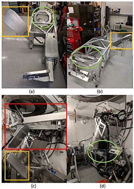
Figure 4. Fabricated TIME mirrors and mechanical sled. The F1 mirror is highlighted in yellow, the cryostat bottom fixture is circled in green, and the K-mirror (K1–K3) is boxed in red. The experiment has begun engineering runs for testing.
Download figure:
Standard image High-resolution imageThe mirror surfaces designed using local optimization guided by human experience and intuition were compared to a local optimization process guided by the parametric fitness function defined in equation (5). (Note: The parametric merit function was defined using the standard optical design merit function editor communicating with customized Matlab function.) The fitness function was used to guide the local optimization in an optimal manner, and a worst-case manner to demonstrate its ability to objectively guide. In all three cases, the same merit function was used for the local optimization process. A smaller merit function means that the design has better satisfied all constraints. The final merit function value in all three cases is shown in table 2, where the optimal fitness function was able to find a lower local minimum than the human designer experience.
Table 2. Overview of the three trials completed to test the objective guidance provided by the fitness function [20]. The same merit function is used in all three cases to evaluate the designs and for local optimization. It is a combination of spot size, Lyot stop quality, telecentricity, and distortion.
| Surface order | Methodology | Merit function value |
|---|---|---|
| K2 P1 P2 C1 | Human intuition | 0.0151 |
| P1 K2 P2 C1 | Fitness (optimal) | 0.0124 |
| P2 C1 K2 P1 | Fitness (worst-case) | 0.0153 |
3. Reconfigurable optical metrology
Many axially non-symmetric, reconfigurable optical systems utilize highly aspheric or freeform optics to balance performance metrics for all possible configurations. Because the systems are reconfigurable, the metrology must also be reconfigured. Similarly, the ever changing needs of custom optics manufacturing demands metrology equipment that is readily reconfigured for each optic.
Deflectometry is a versatile approach to metrology that has a large dynamic range with low uncertainty [24]. The term 'deflectometry' refers to any process for measuring an optical property by characterizing how a ray of light is deflected by the optic [25]. This term was first applied to reflective systems in 1981 by examining Moiré patterns between tilted Ronchi rulings [26], but computer displays soon replaced Ronchi rulings due to their increased flexibility [27].
Modern phase-measuring deflectometry [28] uses many forms of structured illumination [29, 30] to measure a variety of optics from concave to convex and freeform. Deflectometry also adapts to a variety of manufacturing conditions from coarse grinding to finely polished. Its easy reconfigurability is an invaluable asset in optical metrology.
Our focus on deflectometry is based around its wide applicability to a variety of situations, its easy software configuration, and low cost to implement. Although deflectometry is the workhorse application for many reconfigurable optical systems, other solutions such as direct laser tracker measurements and stitching interferometry provide valuable cross-checks in situations where those tools are suitable.
3.1. Large dynamic range infinite deflectometry
Near-flat or convex optical surface metrology using traditional deflectometry often requires an impractical display or light source size, which has been one of the most challenging dynamic range issues in precision deflectometry approaches. In this section, we discuss a method to simplify the metrology setup.
Initially, deflectometry was utilized for testing concave surfaces, or surfaces which are only very slightly convex. This is due to the nature of deflectometry, which requires that a source area is large enough to satisfy a ray path from the source to the full optical aperture area under test, and then into a camera after reflection. Even for extremely large optical surfaces, such as the 8.4 m Giant Magellan Telescope primary mirror segments [31], the required source area can be as small as 220 mm × 40 mm for a full aperture test [32] if the source and camera are placed near the center of curvature of the optic.
For optics with convex surfaces or convex regions, the required source area can range from very large to infinitely large depending on the surface curvature. For reflective optics, it is impossible to place the source and camera at the center of curvature of the optic. To solve the issue of testing challenging optics such as convex optics using deflectometry, a methodology known as infinite deflectometry (ID) achieves a 2π steradian measurement volume [33]. Other systems have tackled this problem but usually rely on a large number of screens [29] which increases the chance for calibration errors and minimizes measurement flexibility.
ID achieves its wide testing range by creating a virtual source enclosure around the test optic. To do this, a source is tilted to create a ramp over the test optic, and a camera is mounted facing down towards the optic. In this configuration, a portion of the optic under test is measurable. To close the loop and measure the full aperture, the test optic is mounted on a precision rotation stage and clocked a fixed interval, which creates a new 'virtual' deflectometry system at each angular position.
By sweeping through the full 2π rotation, screens of the virtual systems create a 'tipi' source enclosure around the optic under test and allow for testing an extreme range of surface slopes, from concave to convex. The basic principle of the ID system, from the physical hardware to the virtual source enclosure, is shown in figure 5.
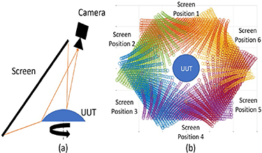
Figure 5. Tilting a planar source screen over a convex optic under test allows for measuring a slice of the optical surface unit under test (UUT) (a). By placing the test optic on a precision rotation stage, the surface can be clocked at fixed intervals through a full rotation. In effect, a new virtual screen and camera are created at each rotated position. The collection of virtual sources creates a 2π steradian measurement volume enclosing the optic allowing for precision metrology over the full aperture (b) (reprinted with permission from [33] © The Optical Society).
Download figure:
Standard image High-resolution imageThe ID system has been used to successfully test both fast convex optics and highly freeform optical surfaces. In one test scenario a fast F/1.26 large convex optic with a 50 mm diameter clear aperture was measured using both an ID system and a commercial interferometer as shown in figure 6.
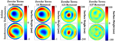
Figure 6. A f/1.26 convex mirror was measured using both the infinite deflectometry method (top row) and a commercial Zygo VerifireTM MST interferometer (bottom row) [33]. Due to uncertainties in both systems for the piston, tip/tilt, and defocus, Zernike terms 1:4 were removed for both reconstruction maps (first column). Additionally, to better compare the surface reconstruction performance across spatial frequencies, Zernike terms 1:6 (second column), 1:21 (third column), and 1:37 (fourth column) were removed for both maps. Reprinted with permission from [33] © The Optical Society.
Download figure:
Standard image High-resolution imageThe interferometer was limited to measuring a 45.29 mm subaperture of the optic. Therefore the reconstructed surface maps of the 45.29 mm diameter common aperture were used for comparison, with the standard Noll-ordered Zernike terms 1:4, 1:6, 1:21, and 1:37 removed. The results demonstrated a strong match between both test methods across all spatial frequencies. After removing Zernike terms 1:37, the interferometer reported 18.48 nm RMS surface height while the ID reconstruction reported 16.26 nm RMS, demonstrating the system can achieve optical quality testing for large, fast, convex optics [33].
It is worth to note that the interferometric and deflectometric approach come with their own advantages and limits supplementing each other. The scanning ID hardware setup costs only a few thousand dollars comparing to the around tens of thousands dollar interferometric system for a similar accuracy. However, the rotational scanning process of the deflectometry takes much longer time (e.g. minutes to hours depending on the unit under test) compared to a single measurement time of interferometry (with limited measurement area). For the stitching interferometry system, the overall measurement time and cost will greatly depend on the overall system approach and architecture.
For a more challenging test, a highly freeform Alvarez lens was measured using the ID system. Because no null optic was available for this surface, and the fringe density with a spherical null exceeded the range of the available commercial interferometers, the surface was cross checked using a KLA-Tencor Alpha-Step D-500 profilometer. The profilometer profile measurement, SP, and the height of the same profile taken from the Alvarez ID map, are reported. The results of the ID reconstruction, the designed Alvarez lens, and the profilometer measurements are shown in figure 7.

Figure 7. An Alvarez lens, a highly freeform optic, was designed with a 6 mm diameter aperture with 17 µm of horizontal coma and—17 µm of trefoil (top right) and manufactured. The final surface generated was measured using the infinite deflectometry (ID) system (top left). To cross check the ID result, a profilometer measurement of a slice of the surface was compared to the same slice from the ID reconstruction map, SID (shown as a black line in the surface map) (top left). The surface height of the profile from the ID measurement and the profilometer were compared (bottom left) and the peak-to-valley (PV) difference was found to be 1.48% of the total PV height across the 6 mm diameter. Reprinted with permission from [33] © The Optical Society.
Download figure:
Standard image High-resolution imageWith these tests, the ID method has proven to be a viable test solution and expands deflectometry to providing optical quality testing for convex optics and highly freeform optics which are traditionally challenging to test.
3.2. Infrared non-null figure metrology
A challenging area of optical fabrication process is the initial shaping process (e.g. generating or grinding). Aggressive processing can quickly remove material, but finding suitable metrology tools to measure the performance is difficult. Most optical metrology systems rely on visible wavelength reflections, but this light is strongly scattered with little useful signal.
Early in the fabrication process, deflectometry with infrared radiation enables optical figuring of a ground surface [34, 35]. This greatly reduces the cost and time for fabricating freeform optics since later polishing stages remove material up to a thousand times slower than during grinding.
Demonstrations of optical figure convergence highlights the usefulness of infrared deflectometry, but understanding the uncertainty in the measurement is important. To do this it is necessary to compare deflectometry measurements to another established metrology system, such as was done with a 6.5 m diameter, rotationally symmetrical conic mirror using long-wave infrared (LWIR,7–12 µm) light [36].
The mirror was clocked in 30° steps to average out systematic errors in the deflectometry system. The computed shape deviation from the ideal conic surface is shown in the left image in figure 8. In this data, power is the largest shape error. The mirror substrate is borosilicate glass, and temperature gradients are known to change the surface figure. The temperature gradient in the mirror was measured simultaneously with the deflectometry data acquisition, and a thermal deformation model was used to compensate for the these effects. The surface error after thermal compensation is shown in the right side of figure 8.
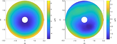
Figure 8. The final averaged surface error map of the 6.5 m diameter aspheric mirror having an RMS error of 3.09 μm (left) and the final map after thermal deformation correction having an RMS error of 1.01 μm (right).
Download figure:
Standard image High-resolution imageFigure 9 shows the difference between the deflectometry and interferometric data. The RMS difference is 0.73 μm, and most of this is power. When power is removed, the total error is 0.33 µm RMS. For comparison, the overall surface shape measured by interferometry shows 0.45 µm RMS of mostly astigmatism. The infrared deflectometry is able to detect that level of astigmatism [37]. To consider high order error the first 37 Zernike terms (Noll order) are subtracted from the discrepancy between deflectometry and interferometry. This data has an RMS value of 0.04 μm which is in good agreement with the 0.02 µm RMS of high spatial frequency features measured by interferometry. While there are some artifacts with 30° spacing due to the clocking of the mirror during testing, the residual is quite small. This shows that infrared deflectometry can accurately measure mid spatial frequencies.

Figure 9. The difference between the final averaged surface error maps of the infrared deflectometry (including thermal bending correction) and null interferometry (including coma correction) for a 6.5 m mirror. Computed RMS error of 0.73 μm (left) and the residual of the difference map with 37 Zernike terms removed having an error of 0.04 μm RMS (right). Figure cedit: [4].
Download figure:
Standard image High-resolution imageThis data shows infrared deflectometry can achieve sub-micron surface accuracy and could be used to polish an optic to a few hundred nanometers RMS error. However, its primary benefit is early in the manufacturing process where material can be removed much faster but other visible-light metrology techniques fail to operate.
On a subsequent project, the infrared deflectometry hardware was reconfigured to guide the grinding process of a different mirror that is 1.5 m diameter. This new mirror was received with spherical surface shape and the grinding process reshapes the surface to be parabolic. Figure 10 shows two images of the surface error during fabrication. On the left is the surface after generation, and before grinding. The mid-spatial frequency structure left by the generating tool is clearly visible. On the right is the surface error during fabrication.
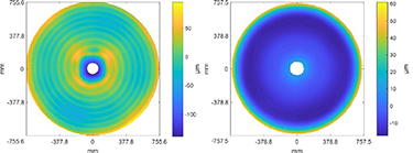
Figure 10. Measured surface errors from a 1.5 m diameter mirror. On the left is an image of the surface error after the spherical surface was generated. On the right is an image of the parabolic surface error after loose abrasive grinding with 40 μm grit.
Download figure:
Standard image High-resolution imageThese two data sets in figure 10 demonstrate two key aspects of infrared deflectometry. The first is that the figure error can be measured very early in the fabrication process. The other is the wide dynamic range and easy reconfigurability of the instrument. The data on the left shows the error of the surface with respect to the sphere that was generated. The data on the right shows the error of the surface with respect to the desired parabola. The only change that was made when switching between the two ideal shapes was in the processing software.
Null solutions, such as LWIR interferometers, are commercially available. However, a large number of custom null optics would be required to measure and guide fabrication of a continuously evolving workpiece. LWIR deflectometry is advantageous for its flexibility during the optical shaping process.
3.3. Temporally modulated, long-wave infrared source
Finding a good thermal source for LWIR light has historically been a limiting factor. The size of a deflectometry source fundamentally limits the dynamic range of measurable slopes and the uniformity directly limits measurement precision, while the signal to noise ratio (SNR) limits the testable range of surfaces. The implications of a low-quality source are particularly insidious for IR deflectometry because the canonical source, a hot scanning tungsten ribbon, is prone to flexing at higher temperatures and longer ribbon lengths, and cannot efficiently scale LWIR spectral flux with higher applied input power.
To extend the reach of infrared non-null measurement to high-sag optics and improve the source SNR, a scalable source architecture called LITMIS, or long-wave infrared time-modulated integrating-cavity source shown in figure 11 was developed [38, 39]. The design utilizes small, self-contained, input nodes which act as pseudo-blackbody radiators when an electric current is applied. LITMIS flexibly places these input nodes into an aluminum integrating cavity, which diffusely emits light from a custom exit aperture.
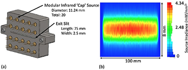
Figure 11. The final optimized LITMIS assembly was modeled in SolidWorks (a). Twenty infrared emitters, EMIRS200 from Axetris, point inside a diffusing cavity which contains a single exit slit, machined from a thin aluminum plate. The optimized design was also modeled in LightTools, where the irradiance at the surface of the box was simulated to assure high uniformity across the exit slit (b) (reprinted with permission from [38] © The Optical Society).
Download figure:
Standard image High-resolution imageAn advantage of this architecture is that the input sources have relatively low thermal mass and can therefore be quickly time modulated. Digital control enables binary modulation of the source so background noise can be subtracted in-situ. Because of the large amount of background thermal radiation present in most test scenarios, up to date background removal is critical for accurate and high SNR testing.
The LITMIS source has been tested against the traditional tungsten ribbon IR deflectometry source, in which a ground glass optic (Glass1500), a machined aluminum disk (AlRoom), and a machined aluminum disk heated to 150 °C (Al150) were all tested using both sources.
The reconstructed surface topology maps of all three test cases are shown in figure 12. The LITMIS source was able to fully test all of the surfaces, achieving 2–5 times larger SNR for the tested optics as compared to the tungsten ribbon. The tungsten ribbon however did not have a sufficient SNR to fully measure the Glass1500 optic. Notably the Al150 sample could not be measured using the ribbon source due to high thermal noise generated, while the LITMIS source provided sufficient data due to the in-situ background removal of the time modulated source.
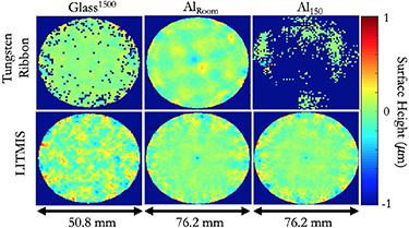
Figure 12. Using both a traditional tungsten ribbon source (top row) and the LITMIS source (bottom row), infrared deflectometry measurements were taken of typical rough optics and standard Zernike terms 1:37 were removed from the reconstructed maps. In the Glass1500 case, SNR from for the tungsten ribbon was too low to test the entire surface, while in the Al150 case, a majority of the surface topology was unavailable due to competitive thermal noise. The LITMIS source was able to entirely test all surfaces. Reprinted with permission from [38] © The Optical Society.
Download figure:
Standard image High-resolution imageThese demonstrations of the LITMIS architecture show that the new source provides a reliable, high SNR source for infrared deflectometry. The ability to create custom emission apertures further adds to the reconfigurability and flexibility of long-wave infrared deflectometry systems.
4. Data monitoring and analysis of reconfigurable systems
When an optical system is actively reconfigured in-situ [40, 41], special data monitoring and analysis tools are required. Maximum performance for the monitoring and analysis requires the computations be fast, accurate and responsive to change.
4.1. Monitoring system for dynamic optical tilt
When you see an image through a mirror, the angle of the mirror determines the area where you can see. If you change the tip-tilt angle of the mirror, the image moves. As a slope-measuring device, configuring deflectometry for orientation measurement is straightforward.
Computationally, a sinusoidal image is created on the source. As the mirror moves, the image motion produces a phase shift in the sinusoidal pattern, and the tip-tilt angle can be calculated from the phase shift. The parameters necessary for the alignment calculation are the distance between the image pattern and the mirror, and the amount of phase shift due to the misalignment.
A proof-of-concept test system comprised of seven hexagonal mirrors is illustrated in figure 13 [42]. Each hexagonal segment can be independently tilted. This type of scenario can occur for active optics systems in large, segmented-mirror telescopes such as the James Webb Space Telescope [43] or the Thirty Meter Telescope [44].
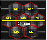
Figure 13. Raw modulated pattern image reflected by seven segmented target hexagonal segmented mirrors (M1–M7) on the camera detector. Reprinted with permission from [42] © The Optical Society.
Download figure:
Standard image High-resolution imageAs a gold-standard reference to compare performance, an autocollimator was aligned with a flat mirror M4 in figure 13, and then the system was oriented to see the reflected pattern through the camera. While scanning the M4 mirror angle, the measured angle from both deflectometry and autocollimator were monitored concurrently and compared. As presented in figure 14 (bottom), the difference between the autocollimator and the deflectometry system is about 0.8 µrad RMS, which is smaller than the noise (error bar) of the data.
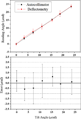
Figure 14. Measurement result for large dynamic range (top) of deflectometry and autocollimator. The difference between the two measurements (bottom) shows less than 0.8 µrad RMS errors. (Note: the error bars represent ±1 σ standard deviation for 30 data measurements). Reprinted with permission from [42] © The Optical Society.
Download figure:
Standard image High-resolution imageTo highlight system adaptability, tip-tilt values were measured in real-time at ∼15 Hz. As shown in figure 15, an actual change in tilt angle on M4 was applied after 5 s.
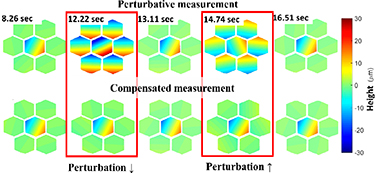
Figure 15. Time sequence snapshots of simultaneous measurement of the seven hexagonal segments, which represent a reconfigurable or dynamic optical system, in figure 13. A different environmental perturbation was introduced around 12 s and 15 s duration (red box). Reprinted with permission from [42] © The Optical Society.
Download figure:
Standard image High-resolution imageMeanwhile, a global perturbation was introduced around 12 s and 15 s into the measurement (two red boxes in figure 15). By monitoring the entire seven segments altogether, the environmental perturbation is clearly recognized as a common motion and compensated for the real M4 orientation change relative to the other segments. The simultaneous measurement capability allows relative orientation data to be distinguished from environmental perturbation [42].
Presently the real-time deflectometry system is limited to measuring tip/tilt alignment only. However the presence of many pixels on each mirror segment, and efficient parameterization methods such as the Chebyshev polynomial functions (section 2.1) open the possibility for higher order shape errors to be measured in real time.
4.2. Incremental electromagnetic thermoforming (IEMTF)
Dynamic deflectometry methods have found several applications in industrial and scientific environments, enabling new processes with potential to enhance time to market as well as production quality and speed. An example of an industrial application under development is the so-called IEMTF or 'induction forming', in which magnetic fields work to heat and shape a workpiece into a compound curve formed in an computer controlled adjustable mold [45, 46]. In this particular application, infrared deflectometry show in figure 16 is proposed to measure the shape quality of the produced panels in real time, being able to adjust the mold and accommodate for incremental steps until achieving the desired final shape.
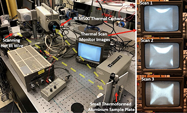
Figure 16. Infrared deflectometry system measuring a small thermoformed aluminum panel for closed-loop manufacturing process feedback.
Download figure:
Standard image High-resolution imageIn this infrared metrology system, the LITMIS (section 3.3) light source can be applied and the illuminating light can be temporarily modulated. The metrology signal (i.e. deflectometry pattern) can be distinguished under varying temperature workpiece conditions during the heating process. This closed loop manufacturing method can produce several different shapes in the same production line with minimal setup changing, and because the shape of the produced pieces is being monitored while it is being thermoformed, real time changes can be performed reducing mold wear, spring back, and other types of effects that may introduce variations in the desired shape quality.
The induction forming has been proposed to produce a variety of complex shaped metallic panels with applications in several industries. Reflector panels for high frequency radio telescopes and satellite downlinks are currently under development in the University of Arizona [47]. Other applications include compound curves for architectural cladding systems, solar power metallic reflectors and different pieces for automotive, marine and aerospace applications.
4.3. Inflatable optical system characterization
As a final example of dynamic measurement, the OASIS (Orbiting Astronomical Satellite for Investigating Stellar Systems) concept is presented. This system utilizes a 20 m inflatable aperture for next-generation terahertz space telescopes [48, 49]. A schematic of the concept is shown in figure 17, and builds on heritage from the 14 m inflatable aperture experiment (IAE) mission.
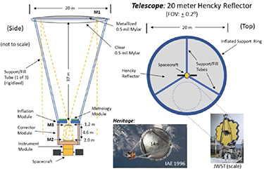
Figure 17. Inflatable 20 m Mylar balloon-based terahertz OASIS telescope concept design and configuration (top and side view).
Download figure:
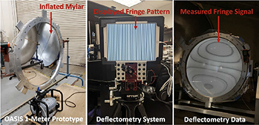
Standard image High-resolution imageAs a technology demonstrator, a 1 m class OASIS Mylar spherical reflector has been successfully manufactured, inflated, and tested at the University of Arizona as shown in figure 18 [49]. The Hencky surface shape and its stability must be calibrated as a function of time, balloon pressure, and thermal environment. Reconfigurable, non-null deflectometry is an effective tool for characterizing the surface variations because the hardware is low cost, provides high spatial resolution and does not require a customized nulling configuration such as a computer generated hologram is needed for interferometry.
Figure 18. A 1 m class inflatable Mylar OASIS prototype tested using the large dynamic range deflectometry measurement and monitoring setup for the on-ground metrology and characterization.
Download figure:
Standard image High-resolution image
The future of very large, space-based telescopes will enable terahertz observations to study the origins of stars, planets, molecular clouds, and galaxies. The OASIS demonstrator is a direct application of a dynamic metrology system's continuous monitoring capability.
5. Summary
Highly flexible and dynamic optical systems such as the TIME instrument, segmented mirror telescope systems, and OASIS concept promise to be key enablers for future scientific discoveries in astronomy. Beyond the need for configurable astronomy systems is the more general need for reconfigurable metrology systems that can readily adapt as sophisticated custom optics are manufactured on demand.
In this paper, we demonstrate advances in all areas of reconfigurable optical system design, metrology and monitoring. From efficient computational functions to deflectometry systems that can measure and improve almost any conceivable optic, the next generation of flexible optical systems is ready for science.
Acknowledgments
The authors would like to thank the Technology Research Initiative Fund (TRIF) Optics/Imaging Program, through the College of Optical Sciences at the University of Arizona, the Post-processing of Freeform Optics project supported by the Korea Basic Science Institute, and the Friends of Tucson Optics (FoTO) Endowed Scholarships in Optical Sciences. The authors would also like to acknowledge the II-VI Foundation Block-Gift Program for helping support general deflectometry research in the Large Optics Fabrication and Testing (LOFT) group.