
Abstract
Neuroscience is home to concepts and theories with roots in a variety of domains including information theory, dynamical systems theory, and cognitive psychology. Not all of those can be coherently linked, some concepts are incommensurable, and domain-specific language poses an obstacle to integration. Still, conceptual integration is a form of understanding that provides intuition and consolidation, without which progress remains unguided. This paper is concerned with the integration of deterministic and stochastic processes within an information theoretic framework, linking information entropy and free energy to mechanisms of emergent dynamics and self-organization in brain networks. We identify basic properties of neuronal populations leading to an equivariant matrix in a network, in which complex behaviors can naturally be represented through structured flows on manifolds establishing the internal model relevant to theories of brain function. We propose a neural mechanism for the generation of internal models from symmetry breaking in the connectivity of brain networks. The emergent perspective illustrates how free energy can be linked to internal models and how they arise from the neural substrate.
Export citation and abstract BibTeX RIS

Original content from this work may be used under the terms of the Creative Commons Attribution 4.0 licence. Any further distribution of this work must maintain attribution to the author(s) and the title of the work, journal citation and DOI.
1. Introduction
Predictive coding is one of the most influential contemporary theories of brain function [1–3]. It is based on the intuition, that the brain operates as a Bayesian inference system, which realizes an internal generative model creating predictions about the outside world. These predictions are continuously compared against sensory input, resulting in prediction errors and updating the internal model (see figure 1). The formulation of brain function in terms of predictive coding is fascinating from the standpoint of theory as it addresses a plethora of profound concepts in diverse fields. This provides the opportunity to link abstract notions such as dynamics, deterministic and stochastic forces, emergence and self-organization [4–6], information, entropy, and free energy [7, 8], stationarity, and many more, within an integrated framework. The integration across domains supports the intuitive understanding of such complex abstractions, even though often, to maintain tractability, not all aspects of the complexity of a given notion are equally captured. As an example, internal models in predictive coding theories use simple models (for instance in decision making, the dynamics is reduced to transitions), which are difficult to generalize to more complex behaviors. This approach is fully justified, when the focus is left on the inference part of the process. Here we wish to do otherwise and actually emphasize the neural basis of the internal model in terms of brain activations, as well as make the link to theories underlying the emergence of complex behavior. Still, given the importance of information theoretic concepts, in particular entropy and free energy, in predictive coding, this endeavor demands their integration with probability distribution functions and the related deterministic and stochastic forces, present in contemporary brain network models (see also [9–11] for related perspectives).
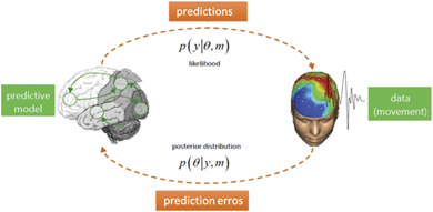
Figure 1. Illustration of the process underlying the Bayesian brain hypothesis as described in the text. The generative model, on the left, embodied in the internal neural dynamics, is updated through information exchange with the external world via perception and action, depicted on the right side of the schematic of the Bayesian inference loop.
Download figure:
Standard image High-resolution imageFree energy has been previously proposed by Karl Friston as a principle for brain function [12–14], which formulates mathematically how adaptive, self-organized systems resist the natural (thermo-dynamical) tendency to disorder. Over time, the free energy principle has grown out of an application of the free energy concept used in the Helmholtz machine, to interpret cortical responses in the context of predictive coding, and has gradually developed into a general principle for intelligent agency, also known as active inference [15]. Both, the Bayesian inference process and the maximum information principle, can be effectively reformulated as a problem of free energy minimization. While these notions of free energy are employed in two related frameworks, they are not exactly identical. Ambiguity may arise from the fact that their general form resembles that of the thermodynamic Helmholtz free energy, however, they follow from two distinct lines of reasoning (see [15] for a detailed discussion). The first is what's termed as 'free energy from constraints' and correspond to the free energy that is minimized in the context of the maximum information principle, representing a trade-off between deterministic constraints and stochastic forces [7]. It is this type of free energy and its constraints, which are our principal consideration here. The other is what is referred to as 'variational free energy' and concerns the Bayesian brain hypothesis. This notion of free energy arises through the reformulation of Bayes' rule as optimization problem that seeks a probability distribution that minimizes a relative entropy (KL-divergence) representing an error of deviation from the exact Bayes' posterior.
The deterministic constraints are expressed in terms of dynamics in the framework of structured flows on manifolds (SFMs) [16, 17], which pertain to low-dimensional dynamical systems arising from networks and are thus a prime candidate for the representation of internal models in brain theories. Correlations of empirically accessible functions such as firing rates, energies, variance and many others contain the link of both, free energy and SFMs, by the agency of probability distributions, which are shaped through the interplay of deterministic and stochastic forces in the system. In his expositions on the meaning of entropy [18, 19], Ilya Prigogine elaborates on the intimate relation of these forces. Here the concept of time goes beyond the notion of repetition and degradation to that of constructive irreversibility, as embodied by a living system perpetuating itself through entropy exchanges with the environment that it is embedded in. Biology is seen to necessitate the inscription of time, as irreversibility, onto matter. In the context of neuroscience, this reminds us of Ingvar's postulate of the brain's ability to simulate 'memories of the future' [20] through its temporally polarized structures, the brain sustains and navigates experiences, of past, present and future, distributed across its different areas.
While, the mathematical formulation for entropy appeared first in the context of classical thermodynamics, relating macroscopic quantities such as heat, temperature and exchange of energy, the statistical mechanics that followed formulated entropy as a function of logarithms of probabilities of the system to be in different possible microscopic states. This latter functional form is identical to that of Shannon's information entropy, in which the probabilities that appear in the expression are those of variables taking on the different possible values (see section 2.2). On a deeper level, as argued by Edwin T Jaynes in 1957, the two concepts of entropy are seen to be synonymous as a measure of uncertainty represented by a probability distribution; in both cases the problem is posed as one of prediction of a probability distribution subject to constraints of observables, and in which the probability distribution which has maximum entropy is the only unbiased choice to be made [7].
This brief discourse on the meaning of entropy finds a theoretical framework in synergetics established by Hermann Haken [4], which formally integrates the mathematical formalisms underlying the emergence of dissipative structures in far-from-equilibrium systems. Nonlinearity and instability give rise to mechanisms of emergence and complexity, whereas entropy and fluctuations lead to irreversibility and unpredictability. The nature of such dynamics then leads naturally to evoking probabilistic concepts, which compensate for our inability to precisely capture individual trajectories of the system. Synergetics has been the driver for translation of these principles to other domains, in particular life sciences and neurosciences. Disentangling the duality of deterministic and stochastic influences, and elaborating on how it arises in the brain, sets the stage for what we aim to achieve here. The goal of this exposition is to unpack these latter intricate relationships in order to consolidate several seemingly disparate frameworks for the modeling of brain dynamics.
With the complementarity of these concepts in mind, and to facilitate accessibility to an audience of diverse backgrounds with an interest in modeling macroscopic brain dynamics, we first step back and review some relevant basic notions of probability and information theory.
2. Information theoretic framework for the brain—modeling system evolution
Edwin T Jaynes emphasized that the great conceptual advance of information theory lies in the insight that there is an unambiguous quantity, the information entropy, which represents the 'amount of uncertainty' through a probability distribution, that intuitively reflects that a broad distribution represents more uncertainty than a sharply peaked one, as well as satisfies all other conditions that make it consistent with this intuition [7]. In absence of any information, the corresponding probability distribution is fully non-informative and the entropy information vanishes. In presence of some deterministic constraints, such as measurements of mean values of physical observables, Lagrange's theory of first kind allows us to solve for the corresponding probability distributions that maximize the information entropy under such constraints (or equivalently minimizes the free energy [7, 12]). It is in this sense that entropic considerations precede the discussion of deterministic influences and the maximum entropy distribution may be asserted by the fact that it respects the consequences of all deterministic forces, but otherwise remains fully non-committal to other influences such as missing information. When entropy is made the principal concepts, the relationships between relevant quantities such as the free energy, probability distribution functions and SFMs are set up naturally, expressing themselves in the real world through correlations, physically accessible through measurement of functions of the system's state variables, and allowing in principle a systematic estimation of all the parameters in the system.
2.1. Predictive coding and its modeling framework
Predictive coding is essentially based on three equations central to its discussion and associated concepts [9, 12–14].


The first equation establishes a reduced form of the Bayesian theorem, expressed in terms of probability distribution functions p, where p(x, y) is the joint probability of the two state variables x and y, and p(y|x) is the conditional probability of the variable y given the state of the variable x. In the Bayesian framework, parameters and state variables have a similar statue in the sense that they can each be described by distributions and enter as arguments into the probability function p. For instance, the probability to jointly find states x and y for a given parameter k is written as p(x, y|k), establishing the likelihood of obtaining a set of data x, y, given a set of parameter values k, which have a prior distribution of p(k). The prior represents our knowledge about the model and the initial values.
The second equation is known as the Langevin equation
1
and establishes the generative model, in which brain activations at the neural source level are represented by the N-dimensional state vector ,
,  are the deterministic influences expressed as an M-dimensional flow vector f depending on the state Q and the parameter k or a set of multiple parameters
  .
.  establishes the fluctuating forces, typically assumed to be Gaussian white noise with ⟨vi
(t)vj
(t')⟩ = cδij
δ(t − t'), where δij
is the Kronecker-delta and δ(t − t') the Dirac function. More general formulations of the influence of noise including multiplicative or colored noise are possible and we here refer the reader to the relevant literature.
establishes the fluctuating forces, typically assumed to be Gaussian white noise with ⟨vi
(t)vj
(t')⟩ = cδij
δ(t − t'), where δij
is the Kronecker-delta and δ(t − t') the Dirac function. More general formulations of the influence of noise including multiplicative or colored noise are possible and we here refer the reader to the relevant literature.
The third equation establishes the observer model and links the source activity Q(t) to the experimentally accessible sensor signals Z(t) via the forward model h(Q) and measurement noise w. For electro-encephalographic measurements, h is the gain matrix established by the Maxwell equations; for functional magnetic resonance imaging measurements, h is given by the neurovascular coupling and the hemodynamic Ballon–Windkessel model. In the present context, the observer model is of no concern, although it is of immense importance in real world applications and plays often the role of a major contaminating factor in problems of model inversion and parameter estimation. We mention these engineering issues here for completeness, but will now for simplicity assume h to be the identity operation with zero measurement noise, thus Z = Q.
Predictive coding relates to a large field of research in behavioral neurosciences [21, 22], in particular ecological psychology [23, 24] devoted to the scientific study of perception-action and dynamical systems. Here James J Gibson stressed the importance of the environment [25], in particular, the perception of how the environment of an organism affords various actions to the organism. This loop of perception-action closely matches the loop of predictions from and update of the internal generative model in predictive coding. A particular nuance emphasized in ecological psychology has been the ecologically available information—as opposed to peripheral or internal sensations—leading to the emergence of the perception-action dynamics. Scott Kelso and colleagues have made major contributions to the formalization of this framework and developed experimental paradigms to test the dynamical properties of the internal models underlying the coordination between the organism and the environment [26–28]. These paradigms were theoretically inspired by Hermann Haken's synergetics [4], which has been foundational for the theories of self-organization. It generated intense research efforts with a strong focus on transitions between states in perception and action, including modeling [29–32] and systematic experimental testing in bimanual and multisensorimotor coordination [33–44]. The approaches were then generalized to larger range of paradigms [45–53] with the goal to extract the principle features of the organism's behavior in interaction with the environment [22]. This large body of work generated substantial evidence for the benefit of dynamical descriptions of behavior, which can be subsumed in the framework of SFMs for functional perception-action variables in behavior (see [48] for a recent review) and the brain [54–56].
2.2. Maximum information principle
Our understanding of the deterministic and stochastic processes determining the discrete value xi of the state variable x is captured by the computation of the corresponding probability distributions pi . Shannon demonstrated the remarkable fact that there exists an information quantity H(p1, ..., pn ), which uniquely measures the amount of uncertainty represented by these probability distributions [8]. In his original proof, he showed that the requirement of three basic conditions, most notably the composition law linking events and probabilities, leads naturally to the following expression
where K is a positive constant. As the measure H corresponds directly to the expression for entropy in statistical mechanics, it is referred to as information entropy [7]. Commonly the discussion of its properties evolves from the perspective of specification of probabilities linked to the amount of information available to an observer. Laplace's principle of insufficient reason assigns equal probabilities to two events in absence of any distinguishing information. This subjective school of thought regards probabilities as expressions of human ignorance, expressing formally our expectation if an event occurs or not. Such thinking is fundamental to theory of predictive coding and its interpretation of cognitive processes generated by the brain. The objective school of thought is rooted in physics and regards probability as an objective property of the event, which can be, in principle, always measured by frequency ratios of events in a random experiment. Here we wish to take an intermediate position in this regard by investigating the deterministic and stochastic processes underlying predictive coding. The reference to deterministic and stochastic forces typically pertains to the language of the objective school, where the subsequent interpretation within the predictive coding framework is part of the subjective school. The generative model in predictive coding represents both types of forces through the Langevin equation and shapes the probability functions, which then provide us with access to this information through the empirical measurement of a function ⟨g(x)⟩. The triangular brackets denote the expectation value
These correlations of g(x), together with the normalization requirement,  , express the constraints provided by deterministic and stochastic influences, within which the information entropy has a maximum. Any other assignment than the maximum of information entropy would introduce another deterministic bias or arbitrary assumption, which by hypothesis we do not have. This insight is the essence of Edwin T Jaynes' maximum information principle [7]. Consequently, we maximize the information entropy H under these constraints by introducing Lagrange parameters λi
in the usual way known from classical mechanics and obtain
, express the constraints provided by deterministic and stochastic influences, within which the information entropy has a maximum. Any other assignment than the maximum of information entropy would introduce another deterministic bias or arbitrary assumption, which by hypothesis we do not have. This insight is the essence of Edwin T Jaynes' maximum information principle [7]. Consequently, we maximize the information entropy H under these constraints by introducing Lagrange parameters λi
in the usual way known from classical mechanics and obtain
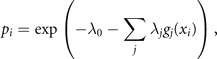
where the expression for the probability distribution is generalized for multiple measured functions gj (xi ) of the event xi . The entropy S of this distribution is maximal and reads
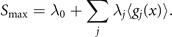
The link between empirical measurements and the maximum information entropy is established by the partition function Z (as in Zustandssumme)
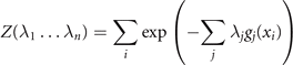
and the relations
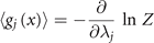

The correlations captured by the empirical measurements ⟨gj (x)⟩ link through these equations to the stationary probability distribution functions and consequently to the generative model (aka deterministic forces) expressed through the Langevin equation. In the following sections, we will provide explicit examples with clear neuroscience relevance.
3. Emergence in self-organizing system—modeling system dynamics
While the above-mentioned frameworks of perception-action dynamics and predictive coding complementarily explain how brain and behavior are shaped through acting on and observing one's environment and self, the framework of SFMs provides a mechanistic picture of how the end result of those shaping processes is embodied. SFMs provides a conceptualization of a spatiotemporal infrastructure in abstract phase space for the constantly evolving internal generative model in the form of spontaneously emerging manifolds of coordinated neural activity that the brain navigates as it experiences and acts on the world. We now briefly discuss the underlying core dynamical systems concepts and the associated mathematical machinery for the investigation of SFMs in the context of brain dynamics.
3.1. Time-scales separation
Emergence in self-organizing systems requires the change of stability of some typically low-dimensional attractor. The system under consideration is nonlinear and high dimensional with N degrees of freedom. In the space spanned by these degrees of freedom, each point is a state vector and represents a potential state of the full system. As time evolves, the state of the system changes and thus traces out a trajectory in state space. The rules that the system follows can be understood as forces that cause the changes of the state vector and define a flow. In order to allow this system to generate low-dimensional behavior, that is, M dimensions withM ≪ N, there must be a mechanism in place that is capable of directing the trajectories in the high-dimensional space toward the lower M-dimensional sub-space. Mathematically, this translates into two flow components that are associated with different time scales: first, the low-dimensional attractor space contains a manifold M, which attracts all trajectories on a fast time scale; second, on the manifold a structured flow F(.) prescribes the dynamics on a slow time scale, where here slow is relative to the collapse of the fast dynamics toward and onto the attracting manifold, as illustrated in figure 2. For compactness and clarity, imagine that the state of the system is described by the N-dimensional state vector Q(t) at any given moment in time t. Then we split the full set of state variables into the components q and s, where the state variables in q define the M task-specific variables linked to emergent behavior in a low-dimensional subspace (the functional network) and theN − M variables of s define the remaining recruited degrees of freedom. Naturally, N is much greater than M and the manifold in the subspace of the variables q has to satisfy certain constraints to be locally stable, in which case all the dynamics is attracted thereto.
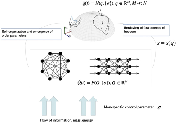
Figure 2. Emergence in a self-organizing dynamical system. External input drives the system out of equilibrium controlled by a control parameter k. Nonlinear interactions in the system lead to the emergence of few macroscopic patterns (order parameters) at critical values of the control parameter. The remaining degrees of freedom are enslaved and follow the evolution of the order parameters.
Download figure:
Standard image High-resolution image3.2. Synergetics
We briefly outline some of the concepts of synergetics first, which will contextualize and aid in better understanding the concepts of SFM. Synergetics is the theory of self-organized pattern formation in open systems (i.e., those that are in contact with the environment through matter, energy, and/or information fluxes) far from thermo-equilibrium that are composed of numerously weakly interacting microscopic elements [4]. Due to the interaction among the microscopic elements, such systems may become organized in spatially as well as temporally ordered patterns that are typically macroscopic in nature and can be described by a limited number of so-called order parameters (or collective variables). Spontaneous switching of brain activity patterns (i.e., non-equilibrium phase transitions) occurs as one macroscopic pattern losses stability while another stable pattern takes hold. The stability of a system's state (or phase) implies that, if perturbed away from it, the system will tend to return to that state. When stability is lost, the system will instead tend to move away from that state and rather switch to another stable state. Close to such points of (macroscopic) instability the time to return increases tremendously. As a result, the macroscopic state evolves rather slowly in response to perturbation, whereas the underlying microscopic components maintain their individual time scale. Consequently, the time scales of their dynamics differ tremendously (time-scales separation). From the perspective of the slowly evolving macroscopic state, the microscopic components change so quickly that they can adapt instantaneously to macroscopic changes. Thus, even though the macroscopic patterns are generated by the subsystems, the former, metaphorically, enslaves the latter [4]. Ordered states can always be described by a very few variables (at least in the close vicinity of a bifurcation) and consequently, the state of the originally high-dimensional system can be summarized by a few or even a single collective variable, the order parameter(s). The order parameters then span the workspace. The circular relationship between the enslaving order parameters and the enslaved microscopic components, which generate the order parameters, is sometimes referred to as circular causality, which effectively allows for a low-dimensional description of the dynamical properties of the system [57]. The notion of circular causality and the emergence of low-dimensional dynamics in self-organizing systems are at the heart of Hermann Haken's synergetics [4].
The mathematical formalism of synergetics can be briefly sketched as follows. An N-dimensional state vector  is defined as a function of time and comprises all state variables of the system. The evolution of the state vector is captured by a nonlinear ordinary differential equation:

where F is a nonlinear function capturing all possible interactions and  is the set of control parameters, which control the state of the system and are time-independent. The nonlinear evolution equation includes the influence of noise υ(t), which shall be considered later, but not here. The state vector and its evolution equations can also be extended to incorporate spatial dependence of the state variables, but it suffices here to consider only spatially discrete systems. For a detailed mathematical treatment see Haken (1983).
The entry point to self-organization and emergence in synergetics is the qualitative change (state transitions) of states of the system on the macroscopic level. A given state typically corresponds to a (stationary) fixed point Q0 or periodic (limit) cycle in state space (see figure 2) and synergetics aims at describing the flow in its local vicinity in state space (figure 3).
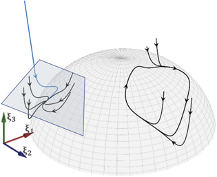
Figure 3. Synergetics and SFMs. In self-organization emerging patterns are constrained to low-dimensional manifolds such as a spherical surface. Criticality in synergetics arises when the flow changes its topology locally (left, rectangular area). Criticality in SFMs is non-local and arises when the flow of the entire manifold is zero.
Download figure:
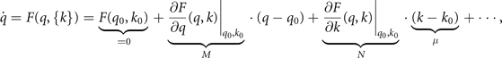
Standard image High-resolution imageThe deviation ɛ(t) from the steady state Q0 is Q(t) = Q0 + ɛ(t) and its time evolution can be approximated by a Taylor expansion of F around the steady state Q0

where  and
and  are the first and second order terms of the Taylor expansion. As the control parameters
  are varied, the system is guided through parameter space and will encounter parameter configurations, for which bifurcations occur, leading to the change of stability of the current state and a major reorganisation of the system on the macroscopic level. The bifurcation point defines the working point k0 and hence a second local constraint, this time in parameter space, next to the working point Q0 in state space. Under these local conditions, at least one of the eigenvalues λ0 of the Jacobian
  becomes zero
2
and allows the application of the local center manifold theorem. It states that a small subset of new variables
becomes zero
2
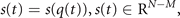
and allows the application of the local center manifold theorem. It states that a small subset of new variables  , the order parameters, arises, which dominate the system dynamics and enslave the remaining variables
  by means of time scale separation, where the order parameters q(t) are slow and the enslaved variables s(t) are fast. In the jargon of synergetics, enslaving means that the intrinsic dynamics of the variables s(t) can be adiabatically eliminated and its long term evolution is expressed as a function of the order parameters, that is s(t) = s(q(t)). This leads then to the reduced description of the emergent dynamics as

where P is a nonlinear function parametrized by  and can be analytically computed from F by use of the decomposition into order parameters and enslaved variables.
3.3. Structured flows on manifolds arising from symmetry breaking
Although synergetics is conceptually not limited to local working points in state space, practically this has always been the case. In biology this has placed an enormous limitation on the utility of the synergetic framework, as the exploration of the flow in state space appears to be a fundamental activity of the organism. To this end, symmetry offers itself as another guiding principle to define the working point in parameter space [9, 16], with the objective to overcome the limitation of confinement to local regions in state space. Dynamical systems with symmetries are called equivariant dynamical systems [59–62], for which group theoretical methods provide a natural language [59, 60]. To demonstrate this, let us consider equation (1) with the state variables formally expressed in  rather than Q(t)
  , for reasons. We return to this point at the end of section 4.2. Further, for simplicity, let us consider only one control parameter k. Let then Γ be a group acting on its solutions. The equation is said to be Γ-equivariant if F commutes with the group action of Γ, that is
  for all γ ∈ Γ. This symmetry shall exist for a critical control parameter value k0. An important consequence of Γ-equivariance is that if a solution q(t) solves the ordinary differential equation, then so does γ ⋅ q(t) for all γ ∈ Γ. If the symmetry is continuous, that is γ ⋅ q = q + δq, then the corresponding group is a Lie group, whose elements have the topology of an M-dimensional smooth manifold M in state space and whose group operation is a smooth function of the elements. Then the stationary solutions of equation (1) span a smooth manifold M, which is defined by

allowing a continuous displacement δq along the manifold. In the case of symmetry breaking, k = k0 + μ, where μ is small, the solutions of the system can be approximated by perturbations of the fully symmetric solution
where M is the smooth invariant manifold of stationary solutions. A zero eigenvalue is associated with the tangent space to M which establishes a time scale hierarchy to the other degrees of freedom as is typically known from synergetics. For full symmetry, k = k0, all points on the manifold are stable fixed points if M is stable. For small symmetry breaking, μ ≪ 1, a slow flow emerges along the manifold, which is slow as compared to the fast dynamics orthogonal to the manifold. These two cases are illustrated in figure 4 for a circular manifold M : 0 = 1 − x2 − y2.
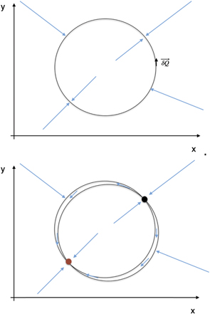
Figure 4. Illustration of a structured flow on circular manifold. Top: the two nullclines for zero-flow in x and in y direction overlap due to full symmetry of the two subsystems. The circular manifold is composed of stable fixed points. Bottom: symmetry breaking, for instance via a coupling between x and y, moves the two nullclines apart and creates a narrow channel of structured flow on the manifold comprising one stable and one unstable fixed point.
Download figure:
Standard image High-resolution imageThe structure of the flow on the manifold is entirely determined by the symmetry breaking through k in N. In the neuroscience context, e.g. in large-scale brain network models, such a symmetry breaking result from variations in the connectivity between brain regions or the local properties of the individual regions. There is no associated immense dimension reduction as we know it from the traditional framework in synergetics, causing a compression from N to M dimensions for the order parameters  . Rather the symmetry is obliged to be defined within a subspace spanned
  , which then is completed by the remaining N − M variables
  as in the traditional synergetic framework. Assuming that these variables are not passing through an instability at the critical point, k = k0, then they can be adiabatically eliminated via enslaving in the usual way and their dynamics is expressed as a function of the order parameters q(t). The difference between the traditional synergetic framework and SFMs is that in the former, the full N-dimensional system is considered allowing the full dimension reduction naturally, whereas in the latter the added constraint needs to be assumed or imposed. These considerations lead us to the following form of system equations:


where  , and
, and  . This set of equations established the basic mathematical framework expressed by SFMs, in which we will develop the basic network equations next.
4. Equivariant dynamics in the brain
The precedent discussion of emerging SFMs is a general one pertaining to all dynamical systems in nature satisfying the constraints. This section makes the link to dynamical systems relevant to neuroscience with the goal to illustrate how SFMs naturally emerge from basic neuroscience networks and create probability distributions in state space.
4.1. Neural mass models show basic 2D dynamics
Neural mass models are reduced mathematical representations of the collective activity of neurons. They are typically derived from a population of neurons, which are represented by coupled point neuron models. Under assumptions about the statistics of the distribution of action potentials and/or coupling between neurons, mean field theory is applied to derive equations of collective variables, capturing the evolution of mean, variance and higher statistical momenta of the population. Notable examples include the Brunel Wang model assuming Poisson distributed spikes [63], Zerlaut et al model using master equation and transfer function formalisms [64], and the Stefanescu–Jirsa model [65, 66] exploiting the heterogeneity of neuronal parameters leading to synchronized clusters of neurons. The mean field derivation of Montbrio et al is particularly attractive from the theoretical perspective [67], because it is exact under the assumption of Lorentzian ansatz. It derives two collective state variables, the mean firing rate r and the mean neuronal membrane potential V. The corresponding phase flows are plotted in figure 5(A), the equations in figure 5(B). These and all other neural mass models have in common that they reduce the mean field dynamics to a low-dimensional representation, often in 2 dimensions. The neural mass dynamics typically comprises a down state corresponding to a low firing rate, an upstate corresponding to a high firing rate, and the capacity to show oscillatory dynamics prevalently in the upstate. Ignoring the oscillatory dynamics for the time being, we can conceptually reduce the co-existing up and down states and their stability changes via bifurcations to the phaseflow of a single variable, x, as illustrated in figure 5(C). Here the phase flow is reduced to the separation of the two stable states, which may lose stability via saddle-node bifurcations under the change of an external control parameter k. This model is mathematically identical to Wong–Wang model, which was derived under adiabatic approximation from the Brunel Wang model. We wish to emphasize that this representation is not specific to the Brunel Wang neural mass model, but captures the essential dynamic features of all neural mass models, that is co-existence of a low- and high-firing state for a range of intermediate control parameter values, loss of the low/high-firing state via bifurcations at high/low values of the control parameter. For these reasons we here use this reduced neural mass as the basic building block of the equivariant brain network model in the next section.
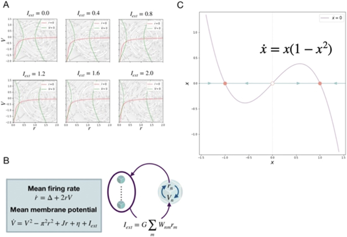
Figure 5. Reduction of neural mass models to a basic one-dimensional form. (A) Two-dimensional Montbrio et al model for various input strengths. (B) Composition of Montbrio et al neural mass model. (C) Reduced one-dimensional neural mass model.
Download figure:
Standard image High-resolution image4.2. Derivation of the equivariant matrix
Symmetry breaking in a network composed of bistable neural masses naturally leads to the creation of SFMs [16]. This can be understood as follows. Let us first consider an intuitive toy network of two nodes with state variables x and y. The underlying equations read


and form a system of coupled neural mass models, where k is the local excitability and v the noise, following the notation of equation (1). Figure 6 shows the phase flow in state space for this situation, illustrating four stable fixed points, one unstable fixed point and four saddle points. The red and the green lines identify the nullclines. The above equations can now be formally rewritten as


where the first term on the rhs represents the same circular invariant manifold as seen in the previous section 3.3. For G = 1, these equations are identical to the uncoupled system. As G varies from 1 to 0, the nullclines change their form continuously from infinity (straight lines) through elliptic to a closed circular shape (see figure 6). G acts as a second control parameter quantifying the degree of mutual connectivity, ranging from fully disconnected (G = 1) to all-to-all coupling (G = 0) topology. For a highly interconnected network, that is G ≈ 0, these intermediate values constrain the phase flow on a closed manifold, centered around the origin, creating a symmetric flow and time scale separation. If other forms of symmetry breaking are introduced, such as regional variance of k or asymmetric connections, then this provides a means of systematically controlling the flow on the manifold.
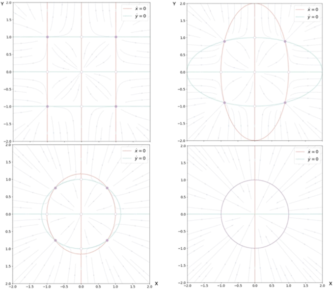
Figure 6. Flow in state space of two nodes under changes of the coupling parameter G. From top left in the sense of the clock:G = 0, 0.25, 0.75, 1.
Download figure:
Standard image High-resolution imageExtending this network to three network nodes, the equations read


where the corresponding phase flow is plotted for G = 0 in state space shown in figure 7. This situation corresponds to the unconnected network nodes as in the previous example. Again, the origin is an unstable fixed point, located symmetrically within a cube comprising 1 unstable fixed point, 8 stable fixed points, separated by 12 saddle points, that are aligned along the nullclines defining the edges of the cube (see figure 7). As connectivity is being established between the three nodes, G reduces to smaller values toward the fully connected network with G = 0. For the latter, the invariant manifold is a 2-sphere, centered at the origin with radius 1 and zero flow.
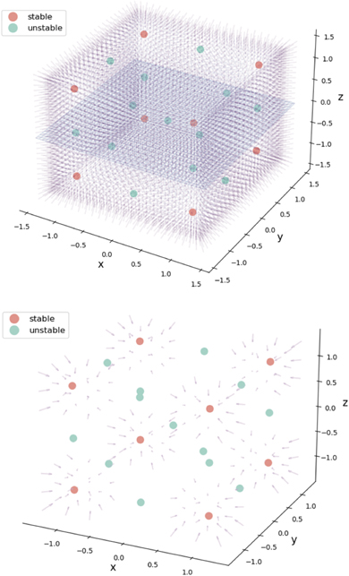
Figure 7. Flow in a network of three uncoupled nodes. A 3 three-dimensional cube spans an equivariant matrix with 1 unstable fixed point in the center (green), 8 stable fixed points (red) and 12 saddle points (green). Upper and lower figure show the same situation with different degrees of detail.
Download figure:
Standard image High-resolution imageThis situation can be formally generalized to a network composed of N basic units
The network establishes an equivariant matrix in N-dimensional state space, in which for the absence of any coupling, 2N
stable fixed points exist, separated by the same number of unstable fixed points, all centered around the origin. As connections are established, the system's phase flow is more and more constrained to the proximity of the (N − 1)-sphere  , which is the manifold M as discussed in section 2.2 and composed entirely of stable fixed points for G = 0, cij
= 1 ∀ i, j, in full analogy to the 2 and 3 dimensional cases. In case of more elaborate symmetry breaking, for instance through the introduction of a connectome, here cij
≠ 1, or variation in regional excitability ki
and local noise vi
, a large range of structured flows can be established on this manifold.
, which is the manifold M as discussed in section 2.2 and composed entirely of stable fixed points for G = 0, cij
= 1 ∀ i, j, in full analogy to the 2 and 3 dimensional cases. In case of more elaborate symmetry breaking, for instance through the introduction of a connectome, here cij
≠ 1, or variation in regional excitability ki
and local noise vi
, a large range of structured flows can be established on this manifold.
Connectome based network modeling has been performed extensively for resting state activity [68–75], but no rigorous theoretical perspective has yet been offered beyond descriptive statistics (such as functional connectivity, functional connectivity dynamics, multiscale entropy) and hypothesized mechanisms (subcriticality, stochastic resonance). The symmetry breaking of the equivariant matrix through the connectome adds an attractive alternative explanation. However, it still lacks an important explanatory argument, as there is no substantial dimension reduction provided by the symmetry breaking of the equivariant matrix. The invariant manifold remains N − 1 dimensional. As discussed in section 3.3 in general, and now here specifically for neuroscience, it poses questions in terms of how such a dimension reduction of the variables Q(t) inN-dimensional space to variables q(t) in M-dimensional space can be accomplished, as M should be much smaller than N.
The following is a possible realisation. In more realistic neuroscience models, the fixed points will not be identical. Generally the down state is more stable than the upstate. Although such differences will inevitably introduce gradients into the flow of the network, it will not suffice to reduce the low-dimensional manifolds that are required for task-specific processes and are known to exist in the human brain activity. Discussions in the literature evoke the possibility of decorrelation as an important mechanism for information processing [76–78] and may here be realized by oscillations in the upstate. Decoupling via frequency separation or averaging is a well known mechanism in dynamical system theory (e.g. rotating wave approximation) and exploited in large-scale brain networks for the organization of synchrony [79] and cross-frequency coupling [80]. Such capacity for oscillatory behavior is an excellent candidate for the purpose of disconnecting an equivariant M-dimensional manifold from its N − M-dimensional complementary subspace with M ≪ N, offering a clear path forward for future scientific investigation.
4.3. Derivation of the probability distribution function and the free energy
The free energy can be seen to mirror the evolution of structured flows on the manifold created by the deterministic features present in the system. In the context of the large scale brain network models, we demonstrated that the symmetry breaking via the connectome qualifies as a candidate mechanism underlying the emergence of these features, thereby establishing the link to biophysical processes such as Hebbian learning and other plasticity mechanisms. The system is then entropically driven by stochastic fluctuations exploring the manifold. Each point on the manifold is associated with a probability distribution. As a limit case in absence of stochastic forces, these distributions are sharply peaked approximating delta-functions and the structured flow is fully deterministic [16]. The link between these deterministic and stochastic influences is the Fokker–Planck equation, which prescribes the temporal evolution of the probability distribution functions [4]. By restricting our attention to the prediction of its stationary properties, the interpretation of the statistical properties is rendered time independent, and we can refer to states, otherwise the interpretation of the state of the system at time t is to be carried out on the basis of measurements performed at time t only.
We wish to illustrate this along a two examples. The first example pertains to the situation previously discussed in section 4.1, in which two nodes were coupled. Let us place the initial focus on only one of the two stable fixed points. We linearize its flow and obtain the following expression
where V(x, y) is the potential, v the noise, y0 a deplacement and β the coupling strength. The deterministic and stochastic influences express themselves in the experimentally accessible correlations, establishing the constraints that need to be satisfied when constructing the probability distribution function p(x, y). The expectation value of a function g(x, y) is ⟨g(x, y)⟩ which can be widely represented by the statistical momenta ⟨x⟩, ⟨y⟩, ⟨x2⟩, ⟨y2⟩, ⟨xy⟩, .... The stationary probability distribution function
is the time independent solution to the Fokker–Planck equation 3
where x1 = x and x2 = y, and N is the normalization constant. It can be expressed by the ansatz

where all the Lagrange multipliers λi
can be estimated explicitly in the usual way from the experimentally accessible correlations ⟨g(x, y)⟩ and the normalization condition  . Without limiting the generality, we can write the above for simplicity assuming λ1 = −1, λ2 = 0 and λ3 = −2β, λ4 = 2y0, λ5 = −1 and obtain

The normalization factor is obtained from the term with λ0. This joint probability distribution function can be formally rewritten to reflect the Bayes theorem and link back to our initial discussion, that is

where Nx , Ny are the normalization constants of p(x|y), p(y). If the two nodes are independent, then naturally the momenta factorize ⟨xy⟩ = ⟨x⟩⟨y⟩ and the deterministic coupling β = 0. The conditional probability p(x|y) becomes independent of y, that is p(x|y) = p(x), and both p(x) and p(y) are fully Gaussian. The expressionF = (x − βy)2/Q is the free energy and intuitively captures the interaction between the nodes as a deformation of the stationary probability density as illustrated in figure 8.
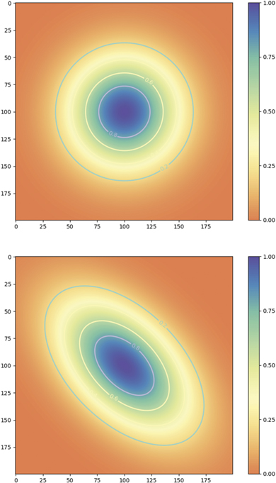
Figure 8. Probability distributions around a stable fixed point in a two-dimensional network of linearly coupled identical nodes with coupling strength β = 1 − G. Top: β = 0. Bottom: β = 0.5.
Download figure:
Standard image High-resolution imageThe second illustrative example comprises the equivariant matrix in section 4.2. For simplicity, we restrain the discussion again to two nodes. Following the same mathematical steps as in the previous example, the potential function for the coupled nodes reads

where β = G − 1 is the coupling strength, with β = 0 for no coupling. With the same arguments as before, we can now write the stationary probability function as p(x, y) = p(x|y)p(y) with
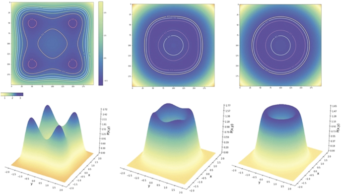
In full analogy, the free energy is explicitly given by F =  and provides an illustrative example of Friston's free energy principle, where the essential deterministic and stochastic features of the correlations between x and y are captured via the interaction term with β. For β = 0 the two nodes are statistically independent and display each a bimodal distribution illustrated in figure 9. Each individual fixed point can be locally approximated by a Gaussian, which can be analytically derived by a Taylor expansion of the full probability density function around the fixed point. As the coupling strength β increases toward 1, the stationary probability distribution changes its shape approaching the circular manifold and structuring its flow on the manifold. Distributions for various β values are plotted in figure 9. Here the structured flow comprises the four stable and four unstable fixed points.
Figure 9. Potential and stationary probability distribution functions in an equivariant network of two nodes. The coupling strength is varied from left to right strength β = 1 − G = 0, 0.75, 1. Top row: potential. Bottom row: probability distributions.
Download figure:
Standard image High-resolution image
5. Final thoughts and conclusions
If we accept the concept of entropy and information as discussed here as the first basic primitive, then what follows naturally from the information theoretic framework, in light of our intuitive understanding of entropy as uncertainty, is the fundamental organization of deterministic and stochastic influences expressed in the shape variations of probability distribution functions. This consequence applies to all systems in nature and not just the brain, which is why Hermann Haken often referred to this as the second foundation of synergetics [4].
Narrowed down to the forces present in brain networks, we linked basic properties of neural masses and networks to the emergence of invariant manifolds in state space, which are the carrier of structured flows known from behavioral neurosciences, in particular ecological psychology and coordination dynamics. The SFMs represent the internal model in predictive coding. This link to behavior is important as it has been regularly called upon to guide research in neuroscience to make it ecologically meaningful. When computing the probability distribution functions explicitly, the free energy appears naturally expressed by the structured flow on the manifold, which in turn is generated by the couplings between the network nodes. During the process of active inference, the brain adjusts these couplings to change the corresponding SFMs (aka the internal model).
Let us bear in mind that these couplings (or more precisely: the coupling parameters) are target for variation under the minimization of free energy in predictive coding on the one hand side, and responsible for the realization of task specific functional architectures in behavior on the other hand side. Unlike the free energy principle which addresses the mechanism of 'how' the network evolves in terms of connectivity and parameters, SFMs instead address the 'what'—'that is, what are the constraints upon the network that need to be satisfied to enable the emergence of a particular flow and manifold' [16]. As such, entropy and free energy can be evoked to explain the evolution of the processes through learning and development, but can also be seen to be at play on the shorter timescales of cognitive performance. Accordingly, the flows on the low-dimensional task-specific manifolds capture, in abstract state space, the mechanistic manifestation of entropy as constructive irreversibility in the brain, and thus, serve as a principal enabling link between neural activity and behavior.
Acknowledgments
We wish to thank Hermann Haken, Karl Friston and Randy McIntosh for many discussions on this topic, as well as Spase Petkoski, Claudio Runfola for discussions and useful comments on an early version of this text. Claudio Runfola and Meysam Hashemi helped with some of the figures and we thank them for their aid. This work is funded through the European Union's Horizon 2020 Framework Programme for Research and Innovation under the Specific Grant Agreement No. 945539 (Human Brain Project SGA3).
Data availability statement
No new data were created or analysed in this study.
Footnotes
- 1
A technically more precise form identifying the underlying calculus can be found for instance in [4]. The here assumed calculus is Ito.
- 2
Positive and negative eigenvalues of the Jacobian are associated with exponentially expanding and contracting flows along local unstable and stable manifolds, respectively, transverse to the center manifold which is associated with the eigenvalues on the imaginary axis [58].
- 3
Note that there exist generalizations of the formalism to nonlinear Fokker–Planck equations addressing complex behaviors like anomalous diffusion. This leads to a free energy-like functional related to non-extensive (Tsallis) entropy functions, e.g., see [81].