


Abstract
We present two algorithms to identify and flag radio frequency interference (RFI) in radio interferometric imaging data. The first algorithm utilizes the redundancy of visibilities inside a UV cell in the visibility plane to identify corrupted data, while varying the detection threshold in accordance with the observed reduction in noise with radial UV distance. In the second algorithm, we propose a scheme to detect faint RFI in the visibility time-channel (TC) plane of baselines. The efficacy of identifying RFI in the residual visibilities is reduced by the presence of ripples due to inaccurate subtraction of the strongest sources. This can be due to several reasons including primary beam asymmetries and other direction-dependent calibration errors. We eliminated these ripples by clipping the corresponding peaks in the associated Fourier plane. RFI was detected in the ripple-free TC plane but was flagged in the original visibilities. Application of these two algorithms to five different 150 MHz data sets from the GMRT resulted in a reduction in image noise of 20%–50% throughout the field along with a reduction in systematics and a corresponding increase in the number of detected sources. However, in comparing the mean flux densities before and after flagging RFI, we find a differential change with the fainter sources (25σ < S < 100 mJy) showing a change of −6% to +1% relative to the stronger sources (S > 100 mJy). We are unable to explain this effect, but it could be related to the CLEAN bias known for interferometers.
Export citation and abstract BibTeX RIS
1. Introduction
At low radio frequencies, below 1 GHz, the radio frequency interference (RFI) environment is quite active and can cause severe degradation in image quality. RFI can increase image noise by up to an order of magnitude above the thermal noise expected for the telescope. The images also usually exhibit widespread systematics in the form of multiple ripples, which increase the detection thresholds of faint objects.
There has been much effort directed toward RFI mitigation and flagging strategies in both hardware (pre-correlation) and software (post-correlation) regimes. Hardware-based techniques typically use either some sort of a reference signal to measure the interference and subtract it from the data (Barnbaum & Bradley 1998; Briggs et al. 2000; Fridman & Baan 2001; Hellbourg et al. 2014) or use specialized hardware such as additional antennas (or antenna arrays) to null sources of interference along certain directions (Van Der Veen & Boonstra 2004; Kocz et al. 2010). Among the software-based tools there are techniques that attempt to excise the RFI from the data i.e., recover the uncorrupted visibilities (Golap et al. 2005; Athreya 2009; Pen et al. 2009; Offringa et al. 2012a) and methods to remove—i.e., flag—the affected data (Bhat et al. 2005; Middelberg 2006; Winkel et al. 2007; Offringa et al. 2010, 2012b). The software methods have an advantage in that they can be applied to both new as well as archival observations.
In general, a single mitigation strategy has not proved to be very effective, as different sources of RFI leave different signatures in the data. Persistent RFI appears as strong fringes in a baseline, and the amplitude and phase of these fringes can change as a function of both time and frequency. Broadband RFI can affect the entire baseline and cause fluctuations in antenna gain and are much more difficult to characterize and eliminate. Intermittent RFI, localized in time and frequency, look like "hotspots" in the visibility data and cause large-scale ripples in the image plane.
We describe here two new methods to identify and flag intermittent RFI, which have consistently yielded high-sensitivity images when applied to a variety of GMRT observations.
2. Description of the Algorithms
The measured visibilities in any polarization in the presence of RFI signal can be written as

where ij are antenna indices,  are the visibilities due to sky emission,
  is correlated RFI,
  is the fringe stopping function (and the only polarization independent factor), and ηij is additive noise in the system. Gi and Gj are the complex antenna gains, which can be affected by strong RFI even if the RFI is uncorrelated.
  will stop the fringe of the cosmic source at the phase center but introduces a corresponding fringe on a stationary (terrestrial) source, like RFI. Athreya (2009) used the form of
  to excise RFI while recovering the visibilities.
VRFI can be orders of magnitude larger than Vsky and vary with time, frequency, and baseline. The second term in the above equation causes poorer solutions during self-calibration and introduce systematic errors in the image.
In this paper, we focus on intermittent RFI, which are localized in the visibility space. These localized hotspots will result in large-scale ripples across the image. We explore two different visibility spaces, viz. the binned UV plane of the entire interferometer and the time-channel (TC) plane of a single baseline, to locate and flag corrupted visibilities. The two algorithms are individually called GRIDflag and TCflag, respectively, and are combined into an integrated RFI flagging package called IPFLAG.
2.1. RFI Flagging in the Gridded UV Plane—GRIDflag
Visibilities sampled by a baseline form a continuous track across the UV plane. The tracks of different baselines are distributed irregularly and usually sparsely. Imaging algorithms compensate for this by interpolating these sampled visibilities onto a regular grid to be able to use the fast Fourier transform (FFT) algorithm (Thompson et al. 2001). This gridded UV plane is fundamental to almost all imaging algorithms, and the sampled cells within the UV grid define the UV coverage of the observation. The size of the UV cell is related to the field of view being imaged. A single baseline will in general contribute multiple visibilities to a particular cell. These multiple visibilities usually lie within a short time interval of each other, unless the observation spans multiple epochs. Multiple baselines may contribute to the same cell, but at different times.
All of the visibility samples within a cell approximately measure the same celestial information, but differ in the RFI environment that they encountered due to different times of observation. We propose to use this dichotomy to identify and flag RFI-affected visibilities.
The first step of the GRIDflag algorithm is to bin the visibilities based on their UV coordinates. The size of a UV-bin is similar in size to the UV cell used while imaging. We assume that in the absence of RFI, the differences between the visibilities in a UV-bin are dominated by system temperature and not source structure. This is valid when applying the scheme to the residual visibility plane obtained after subtracting the strongest sources. Thus, any differences between the visibilities within a UV-bin component that are well in excess of the system noise can be ascribed to RFI. The visibility function must be locally smooth for any realistic sky intensity distribution. Therefore, one can combine data from adjacent UV-bins to calculate statistically secure thresholds to identify RFI.
The standard radio astronomy imaging procedure consists of pre-calibration flagging and several rounds of imaging and self-calibration followed by (often manual) residual visibility flagging procedures available in CASA/AIPS (Greisen et al. 2003; McMullin et al. 2007). Typically, observers using the GMRT 150 MHz band produce images with RMS noise of 1.5–5 mJy beam−1 by using these standard procedures. We have routinely reached below 1 mJy beam−1 using the pre-calibration RfiX procedure (Athreya 2009) to excise persistent broadband RFI. We applied the algorithms described in this paper at the end of this standard procedure. Our recipe is as follows:
- 1.Apply the RfiX algorithm and the standard CASA/AIPS calibration, imaging, and flagging process to obtain the residual visibilities.
- 2.Allot the visibilities into bins in the UV plane. These bins are approximately the same size as the UV-cells used for gridding by imagers. Calculate the robust median and standard deviation (with respect to the median) of all the residual visibilities falling within each UV-bin.
- 3.Partition the UV plane into several annuli and calculate RFI thresholds as a function of UV radius. This is because both RFI and source signals in the residual visibilities tend to decrease with radial distance. The choice of the annulus width is not critical and is decided by the competing requirements of tracking the change in RMS with radius and having sufficient UV-bins within an annulus.
- 4.Use the distribution of medians in an annulus to exclude highly contaminated UV-bins while determining the smoothed median background surface. Note that this will be a function of UV radius.
- 5.The smoothed median surface and the local standard deviation is used to identify RFI-affected data within each UV-bin through any thresholding scheme—we used the visibility RMS to define the threshold. One can set this threshold either using data from within the same UV-bin or by combining other UV-bins in the immediate neighborhood.
- 6.Apply these flags to the original, un-smoothed and un-binned data, and redo the entire process of imaging and self-calibration.
This procedure largely preserves the UV coverage for two reasons: the flagging in each UV-bin is processed separately and in most cases at least a few visibilities in each UV-bin survive the process. Second, this procedure allows for smooth variation of standard deviation even within an annulus. Though we have yet to implement it, the variation of standard deviation may be compensated for by differentially weighting the visibilities.
As a matter of detail, only one-half of the visibility data is recorded, as the other half is simply a Hermitian conjugate. Therefore, the visibilities have to be appropriately conjugated to ensure that they all lie within the same half plane. One will also need to extend the data into a few UV-bins in the other half for statistics at the edge.
We applied this procedure separately and successively for the amplitude, real, and imaginary components in the RR and LL and stokes V polarization modes.
2.2. RFI Flagging in the TC Plane—TCflag
RFI may be identified in the residual visibilities in the TC plane of individual baselines. However, the residual TC plane often has multi-component sinusoidal patterns caused by RFI or by improper subtraction of (strong) sources due to several reasons (e.g., an azimuthally asymmetric antenna primary beam, time dependent pointing error, uncorrected gain fluctuations, etc.). These visibility fringes tend to inflate estimates of the standard deviation, thereby increasing the threshold above which RFI (localized in both time and frequency) can be detected. Therefore, we devised a procedure to eliminate these fringes prior to estimating the sigma threshold for flagging RFI. The scheme is as follows:
- 1.For each baseline and polarization, take a two-dimensional Fourier transform of the TC plane within a window to obtain the group-delay–delay-rate (GD–DR) plane. This window has to be large enough to cover a substantial fraction of the fringe period while being smaller than the period over which the amplitude of the fringe may vary.
- 2.Iteratively sigma clip all components above a threshold in the GD–DR plane, thereby eliminating the corresponding fringes in the TC plane.
- 3.Inverse Fourier transform to obtain the fringe-free TC plane.
- 4.Identify RFI-affected data using any threshold algorithm (e.g., sigma clipping) in the fringe-free TC plane.
- 5.Apply the flags to the original data, and restart the process of imaging and self-calibration.
This procedure works because the signatures of source structure and localized RFI differ in the residual TC and GD–DR planes. Any RFI that is localized in time and frequency will be dispersed over the GD–DR plane, whereas a sinusoidal fringe due to source structure will show up as compact peaks in GD–DR.
Because the fringes in the residual visibilities arise primarily from incorrectly subtracted sources, we tried window sizes of 5–20 minutes, with success. We settled on a window size of 10 minutes for all sources, as it also matched the scan breaks in our data. This value does not need to be finely tuned. If the fringe were to change in amplitude or frequency, this will smear the Fourier signal over several pixels resulting in lower efficiency of RFI detection. However, one can also run this procedure using several windows sizes in decreasing succession. This method aims to remove the fringes associated with improperly subtracted sources in the residual visibilities. The highly efficient, modern FFT algorithms work well for all window sizes; the process of FFT and it's inverse results in discrepancies only of the order of double precision computer numbers (∼10−12).
Finally, this algorithm can in principle be applied at any stage of image processing. Even the presence of real source fringes in TC data will not result in artefacts, as we only modify the flags of the original, raw data.
2.3. Observations and Parameters
All of the observations were done with a bandwidth of 16 MHz in the 150 MHz band and a spectral resolution of 62.5 or 125 kHz. The data was recorded with an integration time of 2s. The flow of analysis is shown in Figure 1.
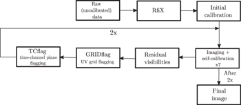
Figure 1. Flowchart describing the data analysis recipe that was used to obtain the final data sets shown in the comparisons below.
Download figure:
Standard image High-resolution imageWe used the following parameters in IPFLAG:
- 1.UV-bin size (GRIDflag): 10λ, from the field of view at 150 MHz.
- 2.Smoothing window for median visibility background (GRIDflag): 5 × 5 bins.
- 3.UV-bin annuli width (GRIDflag): 3, 3 and 6.5 kλ
- 4.Fourier transform window size (TCflag): bandwidth × 10 minutes.
- 5.Fourier peak detection threshold (TCflag): 3 × RMS noise
- 6.RFI threshold (both): 3 × RMS noise
We transferred the RFI flags from IPFLAG to the raw data, and repeated the entire process of imaging, self-calibration, residual flagging, and flag transfer. Finally, the data was again self-calibrated and imaged for the final result (see Figure 1). The final image covers 6 25 × 625 with a pixel size of 4
 5. The sources were extracted from the images using the PyBDSF source finder (Mohan & Rafferty 2015), running with identical parameters across all images.
Stand-alone calibration using the standard CASA/AIPS recipes resulted in flux density scale errors of up to 15%. This becomes important while comparing the absolute noise in an image, though it does not affect the relative change in noise with the application of RFI flagging procedures. We therefore anchored our flux density scale to TGSS-ADR (Intema et al. 2017) using the sources in common with the two observations. The fractional discrepancy in source flux densities is shown in Figure 4. For reasons we do not understand, but which may have to do with something similar to CLEAN bias (Condon et al. 1998; Cohen et al. 2007), we find a flux-dependent fractional discrepancy between TGSS and our flux densities. The fractional discrepancy changes between −0.5% and −9% between sources above and below 100 mJy.
3. Efficacy
We applied IPFLAG to real data from the GMRT at 150 MHz and compared the results with and without the same. The 150 MHz band of the GMRT is important for a variety of astrophysical phenomena but is under-utilized because of the presence of strong RFI. We felt that this comparison using real data would be a more realistic appraisal of the algorithms than simulations with well-behaved noise.
We targeted five fields—VIRMOSC (GMRT observation code: 14RAA01), J1453+3308 (27_063), J1158+2621 (27_063), A2163 (16_259), and 3C286 (TGSS data, Intema et al. 2017).
3C286—A commonly used flux density calibrator source, which is compact and has a flux of 26 Jy at 150 MHz. The field is dominated by point sources with almost no extended emission. However, for reasons that are not understood, this field showed a reduced flux density in TGSS-ADR by ∼25% (see Intema et al. 2017).
VIRMOSC—A field dominated by point sources. The strongest point source in the field is ∼1.7 Jy while it has a single diffuse (4 arcmin) source of 300 mJy.
J1453+3308 and J1158+2621—Double-double radio galaxies, with diffuse outer lobes spanning 4'–7'.
A2163—This is a galaxy cluster with a 14' low surface brightness radio halo.
Figure 2 shows examples of the elimination of the RFI hotspots from the median binned UV plane. Only the upper half of the UV plane is shown in the plot; the lower half is simply the Hermitian conjugate. The band of higher intensity seen at U ≡ [−100 λ, 100 λ] (e.g., J1453+3308 in Figure 2) arises from the inability of the RfiX algorithm to mitigate RFI in regions where the fringe-stop frequency is close to zero.
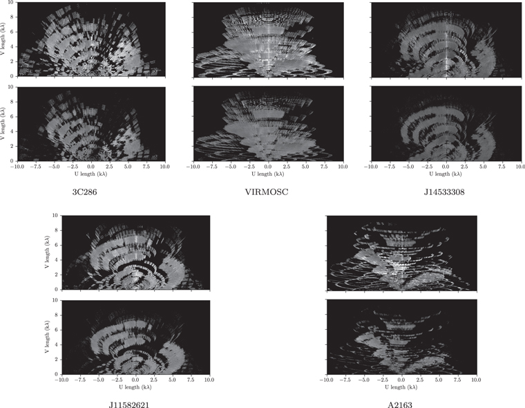
Figure 2. Comparison of the median binned UV plane before and after GRIDflag. The grayscale represents the median flux density in a 10λ × 10λ UV-bin.
Download figure:
Standard image High-resolution imageFigure 3 shows a comparison between TCflag (described here) and existing flagging tools RFlag, TFCrop (both implemented in CASA), and AOFlagger (Offringa et al. 2010, 2012b). Our algorithm TCflag is competitive with the others while using a different procedure to estimate the true noise background.
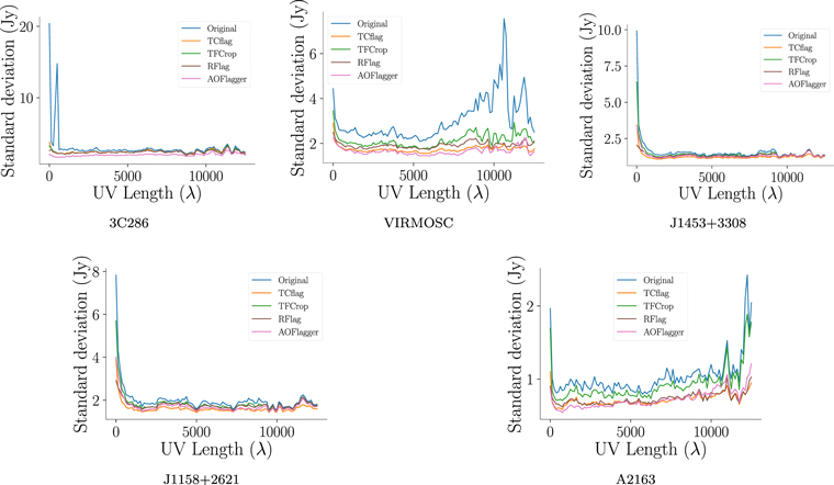
Figure 3. A comparison of the time-channel plane RFI flagging effectiveness of different algorithms. The plots show that TCFlag is competitive with the others while using a different procedure to estimate the true background noise in the time-channel plane of a baseline.
Download figure:
Standard image High-resolution image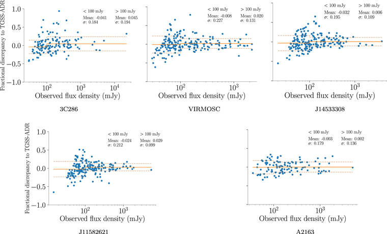
Figure 4. The plots show the fractional flux density discrepancy between our data and TGSS-ADR for point sources common to both. The solid line shows the mean fractional discrepancy (corrected to zero by suitable scaling) and the dashed lines indicate the standard deviation of the scatter for sources above and below 100 mJy.
Download figure:
Standard image High-resolution imageThe total data flagged by IPFLAG was 2.4%–15.7%, and the corresponding loss in UV-bins was 1.2%–3.9%. Table 1 shows that the change in the dirty beam parameters is small before and after IPFLAG, confirming that our procedure did not change the UV coverage despite the loss of a substantial amount of data. We used the same restoring beam before and after IPFLAG in all of our targets. The post imaging comparisons are plotted in Figure 5.
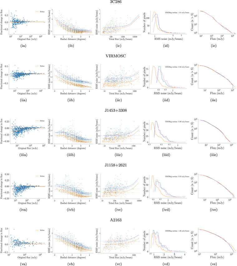
Figure 5. Comparison of images generated using IPFLAG, AOflagger, and with neither. Each row corresponds to a different target, while the five columns show, from left to right, (a) fractional change in flux as a function of original (pre-flagging) flux—only for IPFLAG; the solid line shows the median change separately for the strong (S > 100 mJy), intermediate (25σ < S < 100 mJy) and faint (S < 25σ) sources; (b) image noise as a function of radial distance from the phase center; (c) image noise as a function of neighborhood source flux; (d) histogram of image noise values from across the field; and (e) integral source counts. The results for IPFLAG, AOFlagger, and "Neither" are shown in orange, pink, and blue, respectively. Application of IPFLAG resulted in the detection of fainter sources as evidenced by the extension of source counts to lower flux densities.
Download figure:
Standard image High-resolution imageTable 1. The Effect of IPFLAG on Image Parameters
| Source Name | Without IPFLAG | With IPFLAG | ||||||||
|---|---|---|---|---|---|---|---|---|---|---|
| Major Axis | Minor Axis | NO | σO | Major Axis | Minor Axis | Nf | σf | Flagged Bins % | Flagged Points % | |
| 3C286 | 18.4 | 13.1 | 374 | 1.12 | 18.9 | 13.0 | 403 | 1.01 | 1.2 | 2.4 |
| VIRMOSC | 23.9 | 15.9 | 846 | 0.55 | 25.6 | 15.8 | 949 | 0.42 | 1.7 | 6.4 |
| J1453+3308 | 20.2 | 14.5 | 862 | 0.46 | 18.9 | 14.1 | 870 | 0.38 | 2.7 | 15.7 |
| J1158+2621 | 19.0 | 15.1 | 819 | 0.72 | 18.9 | 14.6 | 844 | 0.55 | 3.9 | 15.5 |
| A2163 | 28.9 | 14.3 | 419 | 1.30 | 31.6 | 15.8 | 493 | 1.06 | 1.5 | 3.9 |
Note. The values of the dirty beam major and minor axes in arcsec, median image noise σo and σf in mJy beam−1, and the number of detected sources No and Nf are listed for each field. We have also listed the percentage of UV-bins lost and visibility data flagged after IPFLAG.
Download table as: ASCIITypeset image
Point source fluxes—The plots in Figure 5(a) show the fractional change in flux density (FCF) as a function of the original (unflagged) flux density. These flux densities were compared before primary beam correction. We analyzed the FCF in three flux density regimes, viz. S > 100 mJy, 25σ < S < 100 mJy, and S < 25σ. 25σ is the flux density above which source counts are typically ∼90% complete (e.g., Intema et al. 2017) and as such defines the limit of the reliability of source catalogs for statistical studies. The FCF ranges from −1% to +6% for the strongest sources. The increase in flux may be expected due to an improvement in calibration after the RFI has been flagged. The mean FCF for intermediate sources is smaller than that for the strong sources by −6% to +1%. This trend in reduction of flux density continues to the faintest sources detected. We saw this reduction with all of the other flaggers as well (AOFlagger, RFlag, and TFCrop), and both of the source detection algorithms used (PyBDSF and aegean; Hancock et al. 2012; Mohan & Rafferty 2015). Suspecting that this discrepancy may be a result of a systematic shift in the background level, we analyzed the residuals in the immediate vicinity of the detected sources before and after flagging but did not detect any such systematic offsets. In summary, this effect is independent of the RFI flagging algorithm used; it does not seem to affect the flux density scale, as the brightest sources are not affected; it must have something to do with the CLEAN algorithm that we use, which comes with CASA. The change in flux density of the intermediate sources is much smaller than the reduction in image noise. At the moment, we have no explanation for this effect, but it may be something similar to the CLEAN bias whose impact is most obvious for the faintest sources (Condon et al. 1998; Cohen et al. 2007). We recall that a similar effect was observed while comparing our flux densities with that of TGSS-ADR in Figure 4.
Image noise as a function of radial distance—In general, the image noise is known to reduce with radial distance. A 200 × 200 pixel box was used to calculate the robust RMS at 625 locations across the image. The plots in column (b) of Figure 5 show both the scatter and the trendline for the unflagged and IPFLAG data; the AOFlagger data is only represented by the trendline in the interest of clarity. The plots show that IPFLAG has reduced the noise all across the image.
Image noise as a function of source flux—Column (c) of Figure 5 shows a plot of the image noise plotted against the cumulative flux density within each of the 625 boxes mentioned earlier. Normally, a higher level of local artefacts is expected in the presence of strong point sources.
Noise Histogram—Column (d) of Figure 5 shows the histogram of the noise across the field. There is a clear shift in the distribution of RMS noise to lower values.
Source Counts—The ultimate metric for image improvement is an increase in source detection at lower flux levels. Figure 5(e) shows that IPFLAG passes this criterion by detecting faint sources to the expected depth. The plot shows the cumulative histogram of the number of sources detected as a function of flux density, i.e., N(> S), which shows clearly that the excess detections come from lower flux densities. Table 1 provides the number of sources detected for each field. In all cases, IPFLAG has resulted in the detection of more sources.
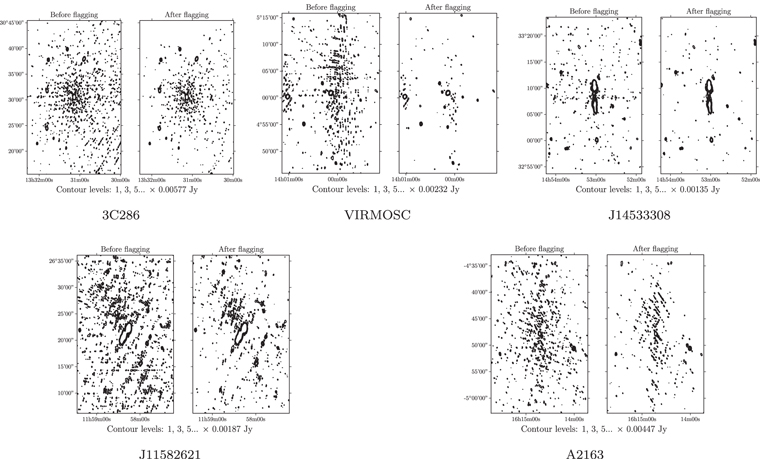
Artefacts—Figure 6 shows the reduction in artefacts in the field after the application of IPFLAG.
Figure 6. A comparison of artefacts in the inner parts of images (1800 × 2700 arcsec2, pixel size 45)—except for the A2163 field where an off-center source is shown—made with and without the application of IPFLAG. The contours levels are indicated below each plot. The unit contour level corresponds to three times the local standard deviation of the IPFLAG image in each case. All fields show a substantial reduction in artefacts on application of IPFLAG.
Download figure:
Standard image High-resolution image
4. Conclusions
The IPFLAG procedures have worked well across a variety of data sets, substantially reducing the image noise and detecting fainter sources. While we tested the algorithms on GMRT data, they should be as effective for any interferometric array in which the UV plane contains a large number of visibility samples.
We are unaware of any other algorithm that approaches RFI flagging in the manner that GRIDflag does. TCflag is similar to several other algorithms like AOflagger, TFcrop, Rflag, etc., which flag localized RFI in the TC plane of an individual baseline while differing in the manner of estimating the background. The combined application of GRIDflag+TCflag, which are components of our RFI pipeline IPFLAG, outperforms the other algorithms. AOFlagger was the closest in terms of performance, and we recognize that a more experienced user of AOflagger may be able to obtain better results by optimizing its many tuneable parameters for GMRT data.
On the other hand, IPFLAG has only six tuneable parameters in total. These values did not require much optimization, and the same values were used for all of the fields tested. In fact, of the six, the UV-bin size selects itself from the field of view, and the three noise thresholds were set to "universal" default values (at 3σ). The width of the UV-annuli was set by simply distributing the visibilities approximately equally across the three annuli used. While the values may require some changes for other frequencies and interferometers, we believe that they will not need to be tuned for different fields.
Upon application of IPFLAG, our images have consistently reached an RMS noise <1 mJy beam−1, with a corresponding increase in source detection; typical GMRT 150 MHz images have hitherto reached an RMS noise of 1.5–5 mJy beam−1, with exceptional effort yielding 0.7 mJy beam−1 (e.g., Ishwara-Chandra et al. 2010). In three of the five images, we have reached an image noise of 0.38–0.55 mJy beam−1, which is only a factor of ∼2 above the theoretical confusion limit. Even in the case of 3C286, an exceptionally bright flux density calibrator, we have reached 1.0 mJy beam−1, and the peak to RMS noise ratio is in excess of 21000, which is unprecedented for GMRT 150 MHz images.
The fact that GRIDflag reduces the loss of UV coverage in the gridded UV plane means that the reduction in RFI is not offset by a corresponding increase in the sidelobes of the synthesized beam. The efficacy of the algorithm depends on the level of redundancy in the gridded visibility plane. The GMRT has good coverage of the shorter spacings, particularly at low frequencies (Swarup et al. 1991), and this coverage is due to get better with the upgraded GMRT (Gupta et al. 2017).
The algorithms also worked at higher frequencies (325 and 610 MHz), but the improvement was not as substantial. We think that this is because of the weaker RFI environment at these frequencies. However, even these weak RFI environments could substantially impact the performance of ultra-deep imaging projects like the MIGHTEE (Jarvis et al. 2017). Furthermore, we believe that GRIDflag is particularly tailored toward multi-epoch observations such as the MIGHTEE, wherein the same UV grids are sampled day after day.
These algorithms will not work in the presence of persistent, broadband RFI. However, other algorithms are available for these situations (e.g., Athreya 2009, used in this paper). We think that the issues that remain to be addressed are the nonisoplanatic ionosphere and an asymmetric antenna primary beam. Applying our algorithms in conjunction with schemes like SPAM (Intema et al. 2009) should yield further improvement of image quality.
We thank the staff of the GMRT who have made these observations possible. GMRT is run by the National Centre for Radio Astrophysics of the Tata Institute of Fundamental Research. Discussions with Drs. Sanjay Bhatnagar and Ishwara-Chandra contributed to this work. We thank the referee for many suggestions that have considerably improved this manuscript.
Facility: GMRT - Giant Meter-wave Radio Telescope.