


ABSTRACT
We compile an updated list of 38 measurements of the Hubble parameter H(z) between redshifts 0.07 ≤ z ≤ 2.36 and use them to place constraints on model parameters of constant and time-varying dark energy cosmological models, both spatially flat and curved. We use five models to measure the redshift of the cosmological deceleration–acceleration transition, zda, from these H(z) data. Within the error bars, the measured zda are insensitive to the model used, depending only on the value assumed for the Hubble constant H0. The weighted mean of our measurements is zda = 0.72 ± 0.05 (0.84 ± 0.03) for H0 = 68 ± 2.8 (73.24 ± 1.74) km s−1 Mpc−1 and should provide a reasonably model-independent estimate of this cosmological parameter. The H(z) data are consistent with the standard spatially flat ΛCDM cosmological model but do not rule out nonflat models or dynamical dark energy models.
Export citation and abstract BibTeX RIS
1. INTRODUCTION
In the standard scenario the currently accelerating cosmological expansion is a consequence of dark energy dominating the current cosmological energy budget; at earlier times nonrelativistic (cold dark and baryonic) matter dominated the energy budget and powered the decelerating cosmological expansion.3 Initial quantitative observational support for this picture came from "lower"-redshift Type Ia supernova (SN Ia) apparent magnitude observations and "higher"-redshift cosmic microwave background (CMB) anisotropy measurements.
More recently, cosmic chronometric and baryon acoustic oscillation (BAO) techniques (see, e.g., Simon et al. 2005; Moresco et al. 2012; Busca et al. 2013) have resulted in the measurement of the cosmological expansion rate or Hubble parameter, H(z), from the present epoch back to a redshift z exceeding 2, higher than currently probed by SN Ia observations. This has resulted in the first mapping out of the cosmological deceleration–acceleration transition, the epoch when dark energy took over from nonrelativistic matter, and the first measurement of the redshift of this transition (see, e.g., Farooq & Ratra 2013a; Farooq et al. 2013a; Moresco et al. 2016).4
H(z) measurements have also been used to constrain some more conventional cosmological parameters, such as the density of dark energy and the density of nonrelativistic matter (see, e.g., Samushia & Ratra 2006; Chen & Ratra 2011b; Chimento & Richarte 2013; Farooq & Ratra 2013b; Ferreira et al. 2013; Akarsu et al. 2014; Bamba et al. 2014; Capozziello et al. 2014; Dankiewicz et al. 2014; Forte 2014; Gruber & Luongo 2014; Chen et al. 2015; Meng et al. 2015; Alam et al. 2016; Guo & Zhang 2016; Mukherjee & Banerjee 2016), typically providing constraints comparable to or better than those provided by SN Ia data, but not as good as those from BAO or CMB anisotropy measurements. More recently, H(z) data have been used to measure the Hubble constant H0 (Verde et al. 2014; Chen et al. 2016a), with the resulting H0 value being more consistent with recent lower values determined from a median statistics analysis of Huchra's H0 compilation (Chen & Ratra 2011a), from CMB anisotropy data (Hinshaw et al. 2013; Sievers et al. 2013; Ade et al. 2015), from BAO measurements (Aubourg et al. 2015; Ross et al. 2015; L'Huillier & Shafieloo 2016), and from current cosmological data and the standard model of particle physics with only three light neutrino species (see, e.g., Calabrese et al. 2012).
In this paper, we put together an updated list of H(z) measurements, compared to that of Farooq & Ratra (2013a), and use this compilation to constrain the redshift of the cosmological deceleration–acceleration transition, zda, as well as other cosmological parameters. In the zda analysis here we study more models than used by Farooq & Ratra (2013a) and Farooq et al. (2013a), now also allowing for nonzero spatial curvature in the XCDM parameterization of the dynamical dark energy case and in the dynamical dark energy ϕCDM model (Pavlov et al. 2013). The cosmological parameter constraints derived here are based on more, as well as more recent, H(z) data than were used by Farooq et al. (2015), and we also explore a much larger range of parameter space in the nonflat ϕCDM model than they did.
We find, from the likelihood analyses, that the  values measured from the H(z) data agree within the error bars in all five models. They, however, depend more sensitively on the value of H0 assumed in the analysis. These results are consistent with those found in Farooq & Ratra (2013a) and Farooq et al. (2013a). In addition, the binned H(z) data in redshift space show qualitative visual evidence for the deceleration–acceleration transition, independent of how they are binned provided that the bins are narrow enough, in agreement with that originally found by Farooq et al. (2013a). Given that the measured zda are relatively model independent, it is not unreasonable to average the measured values to determine a reasonable summary estimate. We find, for a weighted mean estimate, zda = 0.72 ± 0.05 (0.84 ± 0.03) if we assume H0 = 68 ± 2.8 (73.24 ± 1.74) km s−1 Mpc−1.
The constraints on the more conventional cosmological parameters, such as the density of dark energy, derived from the likelihood analysis of the H(z) data here, indicate that these data are quite consistent with the spatially flat ΛCDM model, the standard model of cosmology where the cosmological constant Λ is the dark energy. These H(z) data, however, do not rule out the possibility of dynamical dark energy or space curvature, especially when included simultaneously, in agreement with the conclusions of Farooq et al. (2015). Currently available SN Ia, BAO, growth factor, CMB anisotropy, and other data can tighten the constraints on these parameters, and it will be interesting to study these data sets in conjunction with the H(z) data we have compiled here, but this is beyond the scope of our paper. Near-future data will also result in interesting limits (see, e.g., Podariu et al. 2001a; Pavlov et al. 2012; Santos et al. 2013; Basse et al. 2014).
The outline of our paper is as follows. In the next section, we discuss and tabulate our new H(z) data compilation. In Section 3 we summarize how we bin the H(z) data in redshift space and list binned H(z) data. Section 4 summarizes the cosmological models we consider. In Section 5 we discuss how we compute and measure the deceleration–acceleration transition redshift and tabulate numerical values of zda determined from the H(z) measurements. Section 6 presents the constraints on cosmological parameters, and we conclude in the last section.
2. NEW HUBBLE PARAMETER DATA COMPILATION
In Table 1 we collect 38 Hubble parameter H(z) measurements from Simon et al. (2005), Stern et al. (2010), Moresco et al. (2012), Blake et al. (2012), Zhang et al. (2012), Font-Ribera et al. (2014), Delubac et al. (2015), Moresco (2015), Alam et al. (2016), and Moresco et al. (2016). These data are plotted in the top panel of Figure 1.
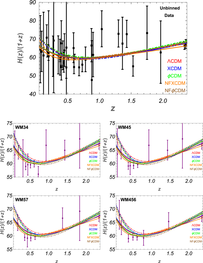
Figure 1. Top panel: 38 H(z) measurements of Table 1. All error bars are 1σ. The left (right) panel in the second row shows the binned H(z) data with 3 or 4 (4 or 5) measurements per bin, combined using weighted mean statistics, listed in Table 2. In the last row, the left (right) panel shows binned H(z) data with 5 or 7 (4, 5, or 6) measurements per bin, combined using weighted mean statistics, listed in Table 2. In all panels, there are five different colored solid (dot-dashed) best-fit model prediction lines for the two H0 priors used in our analyses (see main text for details; NF stands for nonflat).
Download figure:
Standard image High-resolution imageTable 1. Hubble Parameter vs. Redshift Data
| z | H(z) | σH | Reference |
|---|---|---|---|
| (km s−1 Mpc −1) | (km s−1 Mpc −1) | ||
| 0.070 | 69 | 19.6 | 5 |
| 0.090 | 69 | 12 | 1 |
| 0.120 | 68.6 | 26.2 | 5 |
| 0.170 | 83 | 8 | 1 |
| 0.179 | 75 | 4 | 3 |
| 0.199 | 75 | 5 | 3 |
| 0.200 | 72.9 | 29.6 | 5 |
| 0.270 | 77 | 14 | 1 |
| 0.280 | 88.8 | 36.6 | 5 |
| 0.352 | 83 | 14 | 3 |
| 0.380 | 81.5 | 1.9 | 10 |
| 0.3802 | 83 | 13.5 | 9 |
| 0.400 | 95 | 17 | 1 |
| 0.4004 | 77 | 10.2 | 9 |
| 0.4247 | 87.1 | 11.2 | 9 |
| 0.440 | 82.6 | 7.8 | 4 |
| 0.4497 | 92.8 | 12.9 | 9 |
| 0.4783 | 80.9 | 9 | 9 |
| 0.480 | 97 | 62 | 2 |
| 0.510 | 90.4 | 1.9 | 10 |
| 0.593 | 104 | 13 | 3 |
| 0.600 | 87.9 | 6.1 | 4 |
| 0.610 | 97.3 | 2.1 | 10 |
| 0.680 | 92 | 8 | 3 |
| 0.730 | 97.3 | 7 | 4 |
| 0.781 | 105 | 12 | 3 |
| 0.875 | 125 | 17 | 3 |
| 0.880 | 90 | 40 | 2 |
| 0.900 | 117 | 23 | 1 |
| 1.037 | 154 | 20 | 3 |
| 1.300 | 168 | 17 | 1 |
| 1.363 | 160 | 33.6 | 8 |
| 1.430 | 177 | 18 | 1 |
| 1.530 | 140 | 14 | 1 |
| 1.750 | 202 | 40 | 1 |
| 1.965 | 186.5 | 50.4 | 8 |
| 2.340 | 222 | 7 | 7 |
| 2.360 | 226 | 8 | 6 |
References. (1) Simon et al. 2005; (2) Stern et al. 2010; (3) Moresco et al. 2012; (4) Blake et al. 2012; (5) Zhang et al. 2012; (6) Font-Ribera et al. 2014; (7) Delubac et al. 2015; (8) Moresco 2015; (9) Moresco et al. 2016; (10) Alam et al. 2016.
Download table as: ASCIITypeset image
These 38 H(z) measurements are not completely independent. The three measurements taken from Blake et al. (2012) are correlated with each other, and the three measurements of Alam et al. (2016) also are correlated. Also, in these and other cases, when BAO observations are used to measure H(z), one has to apply a prior on the radius of the sound horizon,  , evaluated at the drag epoch zd, shortly after recombination, when photons and baryons decouple. This prior value of rd is generally derived from CMB observations.
Table 1 here is based on Table 1 of Farooq & Ratra (2013a) with the following modifications. We drop older Sloan Digital Sky Survey galaxy clustering H(z) determinations from Chuang & Wang (2013) in favor of the more recent measurements from Alam et al. (2016). We have added the new Moresco et al. (2016) measurements. We have dropped the older Busca et al. (2013) Lyα forest measurement in favor of the newer Font-Ribera et al. (2014) and Delubac et al. (2015) ones. We have also added two new measurements from Moresco (2015).
There are many other compilations of H(z) data available in the literature (see, e.g., Cai et al. 2015; Meng et al. 2015; Duan et al. 2016; Nunes et al. 2016; Qi et al. 2016; Solà et al. 2016; Yu & Wang 2016; Zhang & Xia 2016). We emphasize that our compilation here does not include older, less reliable data, a few with a lot of weight because of anomalously small error bars.
3. BINNING OF HUBBLE PARAMETER DATA
There are two reasons to compute "average" H(z) values for bins in redshift space. First, the weighted mean technique of binning data can indicate whether the original unbinned data have error bars inconsistent with Gaussianity, an important consistency check. Second, data binned in redshift space can more clearly visually illustrate trends as a function of redshift, with the additional advantage of not having to assume a particular cosmological model.
The 38 Hubble parameter measurements in Table 1 are binned to ensure as many measurements as possible per bin, while also retaining as many (narrow) redshift bins as possible. The ideal case is  measurements in each of
  bins. Here we consider about 3–4, 4–5, 4–5–6, and 5–7 measurements per bin. The last four measurements are binned by twos in all but the 4–5–6 measurement per bin case. In all cases, data points in a given bin are not correlated with each other.
After binning the data, we use weighted mean statistics5 to find a representative central estimate for each bin. Following Podariu et al. (2001b), the weighted mean is given by
where H(zi) and σi are the Hubble parameter and one standard deviation of i = 1, 2, 3,..., N measurements in the bin. We also compute the weighted bin redshift using
The associated weighted error is given by
A goodness of fit, χ2, can be found for each bin where the reduced χ2 is

The number of standard deviations that χν deviates from unity (the expected value) is given by

A large Nσ can be the result of non-Gaussian measurements, the presence of unaccounted-for systematic errors, or correlations between measurements. Table 2 lists the weighted mean results for the binned H(z) measurements.
Table 2. Weighted Mean Results for 38 Redshift Measurements
| Bin | N | za | H(z) | H(z) (1σ Range) | H(z) (2σ Range) | Nσ |
|---|---|---|---|---|---|---|
| (km s−1 Mpc −1) | (km s−1 Mpc −1) | (km s−1 Mpc −1) | ||||
| 3 or 4 Measurements per Bin | ||||||
| 1 | 3 | 0.0892 | 69.0 | 59.4–78.5 | 49.9–88.0 | 2.0 |
| 2 | 4 | 0.185 | 76.0 | 73.1–78.9 | 70.2–81.8 | 1.1 |
| 3 | 3 | 0.309 | 80.6 | 71.0–90.2 | 61.5–99.7 | 1.5 |
| 4 | 4 | 0.381 | 81.5 | 79.7–83.4 | 77.9–85.2 | 1.2 |
| 5 | 3 | 0.438 | 85.8 | 80.1–91.5 | 74.3–97.3 | 1.0 |
| 6 | 3 | 0.509 | 90.0 | 88.1–91.9 | 86.3–93.7 | 0.53 |
| 7 | 3 | 0.609 | 96.5 | 94.5–98.4 | 92.6–100 | 0.22 |
| 8 | 3 | 0.720 | 96.6 | 91.8–101 | 87.0–106 | 0.71 |
| 9 | 4 | 0.929 | 129 | 118–140 | 108–151 | 0.066 |
| 10 | 4 | 1.43 | 158 | 149–167 | 140–176 | 0.047 |
| 11 | 2 | 1.83 | 196 | 165–227 | 133–259 | 1.1 |
| 12 | 2 | 2.35 | 224 | 219–229 | 213–234 | 0.88 |
| 4 or 5 Measurements per Bin | ||||||
| 1 | 2 | 0.0846 | 69.0 | 58.8–79.2 | 48.5–89.5 | 1.4 |
| 2 | 5 | 0.184 | 75.9 | 73.1–78.8 | 70.2–81.7 | 1.4 |
| 3 | 5 | 0.377 | 81.5 | 79.7–83.3 | 77.8–85.2 | 2.3 |
| 4 | 5 | 0.427 | 84.6 | 79.8–89.4 | 75.0–94.2 | 1.1 |
| 5 | 5 | 0.518 | 90.1 | 88.3–91.8 | 86.6–93.6 | 0.66 |
| 6 | 4 | 0.628 | 97.2 | 95.3–99.1 | 93.3–101 | 1.2 |
| 7 | 4 | 0.929 | 129 | 118–140 | 108–151 | 0.066 |
| 8 | 4 | 1.43 | 158 | 149–167 | 140–176 | 0.047 |
| 9 | 2 | 1.83 | 196 | 165–227 | 133–259 | 1.1 |
| 10 | 2 | 2.35 | 224 | 219–229 | 213–234 | 0.88 |
| 4, 5, or 6 Measurements per Bin | ||||||
| 1 | 4 | 0.137 | 77.2 | 71.1–83.3 | 64.9–89.5 | 0.85 |
| 2 | 5 | 0.192 | 75.2 | 72.1–78.2 | 69.1–81.2 | 2.3 |
| 3 | 5 | 0.380 | 81.6 | 79.7–83.4 | 77.9–85.2 | 1.5 |
| 4 | 6 | 0.502 | 89.6 | 87.8–91.4 | 86.1–93.1 | 1.1 |
| 5 | 4 | 0.613 | 96.2 | 94.3–98.1 | 92.4–100 | 0.10 |
| 6 | 6 | 0.787 | 106 | 101–112 | 95.8–117 | 1.1 |
| 7 | 6 | 1.46 | 161 | 153–170 | 144–178 | 0.16 |
| 8 | 2 | 2.35 | 224 | 219–229 | 213–234 | 0.88 |
| 5 or 7 Measurements per Bin | ||||||
| 1 | 5 | 0.166 | 75.7 | 72.3–79.0 | 69.0–82.4 | 1.2 |
| 2 | 7 | 0.355 | 80.7 | 79.0–82.4 | 77.2–84.2 | 1.6 |
| 3 | 5 | 0.427 | 84.6 | 79.8–89.4 | 75.0–94.2 | 1.1 |
| 4 | 5 | 0.518 | 90.1 | 88.3–91.8 | 86.6–93.6 | 0.66 |
| 5 | 7 | 0.633 | 97.7 | 95.8–99.6 | 93.9–102 | 0.55 |
| 6 | 5 | 1.37 | 158 | 149–166 | 141–174 | 0.32 |
| 7 | 2 | 1.83 | 196 | 165–227 | 133–259 | 1.1 |
| 8 | 2 | 2.35 | 224 | 219–229 | 213–234 | 0.88 |
Note.
aWeighted mean of z values of measurements in the bin.Download table as: ASCIITypeset image
The last column of Table 2 shows reasonably small Nσ for all binnings, thus suggesting that the error bars of the H(z) data of Table 1 are not inconsistent with Gaussianity. As in Farooq et al. (2013a), we find that the cosmological constraints that follow from the weighted mean binned data are almost identical to those derived using the unbinned data, while the median statistics binned data typically result in somewhat weaker constraints. A possible reason for this could be that some of the unbinned H(z) data error bars might be a bit larger than they really should be. This would be consistent with the low reduced χ2 shown in the last line of Table 1 in Chen et al. (2016a).
The binned data are plotted in the four lower panels of Figure 1. It is reassuring that, independent of the binning used, all the binned data sets show clear visual qualitative evidence for the cosmological deceleration–acceleration transition, as in Farooq et al. (2013a). This is model-independent qualitative evidence for the existence of the cosmological deceleration–acceleration transition. We shall see, in Section 5, that all cosmological models we use in the analysis of the H(z) data to measure zda result in zda values that overlap within the error bars (for a given H0 prior). This is additional model-independent evidence for the presence of the deceleration–acceleration transition.
4. COSMOLOGICAL MODELS
In this section we briefly describe the five models we use to analyze the H(z) data. These are the ΛCDM model, which allows for spatial curvature and where dark energy is the cosmological constant Λ (Peebles 1984), and the ϕCDM model, in which dynamical dark energy is represented by a slowly evolving scalar field ϕ (Peebles & Ratra 1988; Ratra & Peebles 1988). We also consider an incomplete, but popular, parameterization of dynamical dark energy, XCDM, where dynamical dark energy is represented by an X-fluid. In the ϕCDM and XCDM cases, we consider both spatially flat and nonflat models (Pavlov et al. 2013).
In the ΛCDM model with spatial curvature the Hubble parameter is

where we have made use of  to eliminate the current value of the space curvature energy density parameter in favor of the current value of the nonrelativistic matter energy density parameter, Ωm0, and the cosmological constant energy density parameter, ΩΛ. Here
  are the two cosmological parameters that conventionally characterize ΛCDM, and H0 is the value of the Hubble parameter at the present time and is called the Hubble constant.
It has become fashionable to parameterize dynamical dark energy as a spatially homogeneous X-fluid, with a constant equation-of-state parameter,  (here pX and ρX are the pressure and energy density of the X-fluid, respectively). For the spatially flat XCDM parameterization, using
  (where ΩX0 is the current value of the X-fluid energy density parameter), we have
In this spatially flat case the two cosmological parameters are  . The XCDM parameterization is incomplete as it cannot describe the evolution of energy density inhomogeneities. In the nonflat XCDM parameterization case,
  is the third free parameter and
where the three cosmological parameters are  . ϕCDM is the simplest, most complete, and most consistent dynamical dark energy model. Here dark energy is modeled as a slowly rolling scalar field ϕ with, e.g., an inverse-power-law potential energy density
  , where mp is the Planck mass and α is a non-negative parameter that determines the coefficient κ(mp, α) (Peebles & Ratra 1988). The equation of motion of the scalar field is

where an overdot represents a time derivative and a is the scale factor. For the spatially flat ϕCDM model

where the time-dependent scalar field energy density parameter is
In this case the two cosmological parameters are  . In the nonflat ϕCDM model
and the three cosmological parameters are  .
.
Solving the coupled differential equations of motion allows for a numerical computation of the Hubble parameter  (Peebles & Ratra 1988; Samushia 2009; Farooq 2013; Pavlov et al. 2013).6
In Section 6 we use these expressions for the Hubble parameter in conjunction with the H(z) measurements in Table 1 to constrain the cosmological parameters of these models. In our analyses here we study the following parameter ranges: 0 ≤ Ωm0 ≤ 1, 0 ≤ ΩΛ ≤ 1.4, −2 ≤ ωX ≤ 0, 0 ≤ α ≤ 5, and −0.7 ≤ ΩK0 ≤ 0.7 for nonflat XCDM and −0.4 ≤ ΩK0 ≤ 0.4 for nonflat ϕCDM (which is double the ΩK0 range used in Farooq et al. 2015).
5. COSMOLOGICAL DECELERATION–ACCELERATION TRANSITION REDSHIFT
At the current epoch, dark energy dominates the cosmological energy budget and accelerates the cosmological expansion. At earlier times nonrelativistic (baryonic and cold dark) matter dominated the energy budget and the cosmological expansion decelerated. The cosmological deceleration–acceleration transition redshift, zda, is defined as the redshift at which  , in the cosmological model under consideration.
  is proportional to the active gravitational mass density, the sum of the energy densities and three times the pressure of the constituents.
For ΛCDM, setting  , we find
For the case of the spatially flat XCDM parameterization

while for nonflat XCDM
For the spatially flat ϕCDM model, defining the time-dependent equation-of-state parameter for the scalar field
the redshift zda (Ωm0, α) is determined by numerically solving

where  . In the nonflat ϕCDM model zda (Ωm0, α, ΩK0) is determined by numerically solving the same equation, but now setting
  .
.
To compute the expected values  and
and  for the two-parameter models, we use
Here  is the H(z) data likelihood function after marginalization over the Gaussian H0 prior in the two-parameter model under consideration, as explained in Farooq et al. (2013b, 2015), but this time accounting for the nondiagonal correlation matrices of the Blake et al. (2012) and Alam et al. (2016) measurements, which have a small effect.
  depends only on the model parameters
  for ΛCDM,
  for flat XCDM, and
  for flat ϕCDM. The generalization for the three-parameter models is straightforward. The standard deviation in zda is computed from the standard formula
  . The results of this computation are summarized in Table 3.
Table 3. Deceleration–Acceleration Transition Redshiftsa
| Model | h Priorb | BFc |

|
 d d
|
 e e
|
|---|---|---|---|---|---|
| 0.68 ± 0.028 | Ωm0 = 0.23 | 22.4 | 0.723 ± 0.089 | 0.690 ± 0.096 | |
| ΛCDM | ΩΛ = 0.60 | ||||
| 0.7324 ± 0.0174 | Ωm0 = 0.25 | 24.2 | 0.832 ± 0.055 | 0.781 ± 0.067 | |
| ΩΛ = 0.78 | |||||
| 0.68 ± 0.028 | Ωm0 = 0.26 | 22.5 | 0.753 ± 0.091 | 0.677 ± 0.097 | |
| Flat XCDM | ωX = −0.86 | ||||
| 0.7324 ± 0.0174 | Ωm0 = 0.24 | 23.9 | 0.813 ± 0.062 | 0.696 ± 0.082 | |
| ωX = −1.06 | |||||
| 0.68 ± 0.028 | Ωm0 = 0.27 | 22.9 | 0.703 ± 0.104 | 0.724 ± 0.148 | |
| Flat ϕCDM | α = 0.50 | ||||
| 0.7324 ± 0.0174 | Ωm0 = 0.25 | 25.2 | 0.885 ± 0.056 | 0.850 ± 0.116 | |
| α = 0 | |||||
| 0.68 ± 0.028 | Ωm0 = 0.15 | 21.9 | 0.684 ± 0.117 | ⋯ | |
| ωX = −1.68 | |||||
| Nonflat XCDM | ΩK0 = 0.45 | ||||
| 0.7324 ± 0.0174 | Ωm0 = 0.13 | 20.3 | 0.709 ± 0.090 | ⋯ | |
| ωX = −2 | |||||
| ΩK0 = 0.41 | |||||
| 0.68 ± 0.028 | Ωm0 = 0.23 | 22.6 | 0.690 ± 0.118 | ⋯ | |
| α = 0 | |||||
| Nonflat ϕCDM | ΩK0 = 0.18 | ||||
| 0.7324 ± 0.0174 | Ωm0 = 0.25 | 25.0 | 0.853 ± 0.053 | ⋯ | |
| α = 0 | |||||
| ΩK0 = −0.03 | |||||
Notes.
aEstimated using the unbinned data of Table 1. bHubble constant in units of 100 km s−1 Mpc−1. cBest-fit parameter values. dComputed using Equations (13)–(18) of this work. eThe deceleration–acceleration transition redshift in the model, as computed in Table 1 of Farooq et al. (2013a). Note that the best-fit cosmological parameter values found in Farooq et al. (2013a) differ from those found here and listed in this table.Download table as: ASCIITypeset image
Table 3 shows best-fit cosmological parameter values and the corresponding minimum χ2 for the five different cosmological models and for the two Gaussian H0 priors. The second-to-last column in Table 3 shows the average deceleration–acceleration transition redshift with corresponding standard deviation for each model. It is very reassuring that the zda values we measure in the five different models (for a given H0 prior) overlap reasonably well. (The main effect on the measured zda value is the assumed H0 prior value.) Given that the measured zda are almost independent of the other model parameters, within the errors, we may conclude that to leading order we have measured a model-independent zda value. However, it is useful to have a single summary value for this cosmological parameter.
By taking the simple average of the penultimate column zda values and computing the population standard deviation for the five values in this column, we find zda = 0.71 ± 0.03 (0.82 ±0.06) for  (73.24 ± 1.74) km s−1 Mpc−1. Using all 10 zda values in the penultimate column of Table 3, we find zda = 0.76 ± 0.07.
A more reliable summary value of the deceleration–acceleration transition redshift is determined from a weighted mean analysis. Using Equations (1)–(3), we find zda = 0.72 ± 0.05 (0.84 ± 0.03) for  (73.24 ± 1.74) km s−1 Mpc−1, and using all 10 values in the penultimate column of Table 3, we get zda = 0.80 ± 0.02. By looking at the fourth and fifth columns of Table 3, it appears that all five models discussed here fit better with the lower value of H0, while the uncertainty in zda is more sensitive to
  .
.
These results are listed in Table 4 and compared with the previously computed summary values of Farooq et al. (2013a). Note that only three models (ΛCDM, flat XCDM, and flat ϕCDM) were considered in Farooq et al. (2013a). Here we also consider nonflat XCDM and nonflat ϕCDM. We see that there is good agreement between the old and new weighted mean zda for h = 0.68, less so for h = 0.7324. From Table 4 we see that for a given H0 the weighted average values of zda for all five models and for the two sets of (non-nested) triplets of models agree to within the error bars.
Table 4. zda Summary
| Averages | h ± σh = 0.68 ± 0.028a | h ± σh = 0.7324 ± 0.0174a | Totalb | |||
|---|---|---|---|---|---|---|
| Herec | Previousd | Herec | Previousd | Herec | Previousd | |
| Simple averages | 0.71 ± 0.03 | 0.70 ± 0.02 | 0.82 ± 0.06 | 0.78 ± 0.06 | 0.76 ± 0.07 | 0.74 ± 0.06 |
| Weighted averages | 0.72 ± 0.05 | 0.69 ± 0.06 | 0.84 ± 0.03 | 0.76 ± 0.05 | 0.80 ± 0.02 | 0.74 ± 0.04 |
| Simple averages from | 0.73 ± 0.02 | ⋯ | 0.84 ± 0.03 | ⋯ | 0.78 ± 0.06 | ⋯ |
| ΛCDM and flat models | ||||||
| Weighted averages from | 0.73 ± 0.05 | ⋯ | 0.85 ± 0.03 | ⋯ | 0.81 ± 0.03 | ⋯ |
| ΛCDM and flat models | ||||||
| Simple averages from | 0.70 ± 0.02 | ⋯ | 0.80 ± 0.06 | ⋯ | 0.75 ± 0.07 | ⋯ |
| nonflat models | ||||||
| Weighted averages from | 0.70 ± 0.06 | ⋯ | 0.82 ± 0.04 | ⋯ | 0.79 ± 0.03 | ⋯ |
| nonflat models | ||||||
Notes.
aHubble constant in units of 100 km s−1 Mpc−1. bCombination of results from both H0 priors. cEstimated using the unbinned data of 38 H(z) measurements from Table 1. dResults from Farooq et al. (2013a). We have corrected typos in that paper here.Download table as: ASCIITypeset image
6. COSMOLOGICAL PARAMETER CONSTRAINTS
In this section, we use the 38 Hubble parameter measurements (over 0.07 ≤ z ≤ 2.36) listed in Table 1 to determine constraints on the parameters of the five different cosmological models. We use the technique of Farooq et al. (2015) to find constraints on (Ωm0, ΩΛ) in the ΛCDM model, (Ωm0, ωX) for the spatially flat XCDM parameterization, (Ωm0, α) in the spatially flat ϕCDM model,  for the XCDM parameterization with space curvature, and
  in the ϕCDM model with space curvature. For the H(z) cosmological test, cosmological parameter constraints depend on the value of the Hubble constant (see, e.g., Samushia et al. 2007). We use two different Gaussian priors for the Hubble constant; the lower value is 68 ± 2.8 km s−1 Mpc−1, and the higher is 73.24 ± 1.74 km s−1 Mpc−1. The lower value is from a median statistics analysis (Gott et al. 2001) of 553 measurements of H0 tabulated by Huchra (Chen & Ratra 2011a). It agrees with earlier median statistics estimates of H0 from smaller compilations (Gott et al. 2001; Chen et al. 2003) and is consistent with a number of other recent determinations of H0 from Wilkinson Microwave Anisotropy Probe, Atacama Cosmology Telescope, and Planck CMB anisotropy data (Hinshaw et al. 2013; Sievers et al. 2013; Ade et al. 2015; Addison et al. 2016), from BAO measurements (Aubourg et al. 2015; Ross et al. 2015; L'Huillier & Shafieloo 2016), and from Hubble parameter data (Chen et al. 2016a), as well as with what is expected in the standard model of particle physics with only three light neutrino species given current cosmological data (see, e.g., Calabrese et al. 2012). The higher value is a relatively local measurement, based on Hubble Space Telescope data (Riess et al. 2016). It is consistent with other recent local measurements of H0 (Riess et al. 2011; Freedman et al. 2012; Efstathiou 2014).
We compute the likelihood function  for the models under discussion using Equation (18) of Farooq et al. (2013b) for the ranges of the cosmological parameters listed at the end of Section 4. We need these likelihood functions for the zda computation of the previous section, which is the main result of the paper. In this section, we use these likelihood functions to constrain cosmological parameters such as the dark energy density.
For the two-parameter models, maximizing the likelihood function  is performed by minimizing the corresponding
 ![${\chi }^{2}({\boldsymbol{p}})\equiv -2\mathrm{ln}[{ \mathcal L }({\boldsymbol{p}})]$](https://content.cld.iop.org/journals/0004-637X/835/1/26/revision1/apjaa4e43ieqn39.gif) following the procedure of Farooq et al. (2015). The corresponding minimum values of χ2 and best-fit parameter values for the two-parameter models are summarized in Table 3. The 1σ, 2σ, and 3σ confidence contours are computed following the procedure of Farooq et al. (2015), and results are shown in Figure 2. The generalization of this procedure for the three-parameter models is straightforward, and best-fit three-dimensional parameter values and minimum χ2 are also summarized in Table 3.
following the procedure of Farooq et al. (2015). The corresponding minimum values of χ2 and best-fit parameter values for the two-parameter models are summarized in Table 3. The 1σ, 2σ, and 3σ confidence contours are computed following the procedure of Farooq et al. (2015), and results are shown in Figure 2. The generalization of this procedure for the three-parameter models is straightforward, and best-fit three-dimensional parameter values and minimum χ2 are also summarized in Table 3.
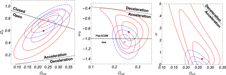
Figure 2. The three panels (from left to right) show 1σ, 2σ, and 3σ red solid (blue dot-dashed) constraint contours for the lower (higher) H0 prior, for ΛCDM, flat XCDM, and flat ϕCDM, respectively. Red filled (blue open) circles are the best-fit points for the lower (higher) H0 prior. The straight dashed lines in the left and middle panels correspond to spatially flat ΛCDM models, the dotted lines demarcate zero-acceleration models, and the shaded area in the upper left-hand corner of the left panel is the region for which there is no big bang. For quantitative parameter best-fit values and ranges see Tables 3 and 6.
Download figure:
Standard image High-resolution imageFor the three-parameter models we next compute three two-dimensional likelihood functions by marginalizing the three-dimensional likelihood function over each of the three parameters (assuming flat priors) in turn. These three two-dimensional likelihood functions are maximized as above, and the corresponding best-fit parameter values and minimum χ2 are listed in Table 5. The confidence contours for these two-dimensional likelihood functions are shown in Figure 3 for the nonflat XCDM parameterization and in Figure 4 for the nonflat ϕCDM model.
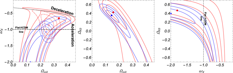
Figure 3. The three panels (from left to right) show 1σ, 2σ, and 3σ two-dimensional constraint contours for the three-parameter, nonflat XCDM parameterization, computed after marginalizing over each of the three parameters in turn. Red (blue) solid lines are for the lower (higher) H0 prior. Left, middle, and right panels correspond to marginalizing over ΩK0, ωX, and Ωm0, respectively. Red (blue) filled circles are the best-fit points for the lower (higher) H0 prior. Red (blue) dot-dashed lines in the left panel are 1σ, 2σ, and 3σ constraint contours for the lower (higher) H0 prior for spatially flat XCDM (see the middle panel of Figure 2). For quantitative parameter best-fit values and ranges see Tables 3, 5, and 7.
Download figure:
Standard image High-resolution image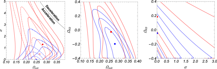
Figure 4. The three panels (from left to right) show 1σ, 2σ, and 3σ two-dimensional constraint contours for the three-parameter, nonflat ϕCDM model, computed after marginalizing over each of the three parameters in turn. Red (blue) solid lines are for the lower (higher) H0 prior. Left, middle, and right panels correspond to marginalizing over ΩK0, α, and Ωm0, respectively. Red (blue) filled circles are the best-fit points for the lower (higher) H0 prior. Red (blue) dot-dashed lines in the left panel are  , 2σ, and 3σ constraint contours for the lower (higher) H0 prior for the spatially flat ϕCDM model (see the right panel of Figure 2). For quantitative parameter best-fit values and ranges see Tables 3, 5, and 7.
Download figure:
Standard image High-resolution image
Table 5. Two-dimensional Best-fit Parameters for Three-parameter, Nonflat Models
| Model | h Priora | Marginalized Parameter | BFb |

|
|---|---|---|---|---|
| 0.68 ± 0.028 | ΩK0 | Ωm0 = 0.38 | 25.3 | |
| ωX = −0.64 | ||||
| ωX | Ωm0 = 0.16 | 22.5 | ||
| ΩK0 = 0.43 | ||||
| Ωm0 | ωX = −1.80 | 27.3 | ||
| Nonflat XCDM | ΩK0 = 0.47 | |||
| 0.7324 ± 0.0174 | ΩK0 | Ωm0 = 0.13 | 25.0 | |
| ωX = −2 | ||||
| ωX | Ωm0 = 0.15 | 22.1 | ||
| ΩK0 = 0.39 | ||||
| Ωm0 | ωX = −2 | 26.8 | ||
| ΩK0 = 0.41 | ||||
| 0.68 ± 0.028 | ΩK0 | Ωm0 = 0.28 | 25.7 | |
| α = 1.33 | ||||
| α | Ωm0 = 0.26 | 22.4 | ||
| ΩK0 = −0.02 | ||||
| Ωm0 | α = 0.01 | 28.7 | ||
| Nonflat ϕCDM | ΩK0 = 0.19 | |||
| 0.7324 ± 0.0174 | ΩK0 | Ωm0 = 0.25 | 29.0 | |
| α = 0.01 | ||||
| α | Ωm0 = 0.28 | 26.6 | ||
| ΩK0 = −0.19 | ||||
| Ωm0 | α = 0.01 | 31.6 | ||
| ΩK0 = −0.04 | ||||
Notes.
aHubble constant in units of 100 km s−1 Mpc−1. bBest-fit parameter values.Download table as: ASCIITypeset image
To get two one-dimensional likelihood functions from each of the two-dimensional likelihood functions, we marginalize (with a flat prior) over each parameter in turn. We then determine the best-fit parameter values by maximizing each one-dimensional likelihood function and compute 1σ and 2σ intervals for each parameter in each model and for both H0 priors. The best-fit parameter values and 1σ and 2σ intervals are given in Table 6 for the two-parameter models and in Table 7 for the three-parameter models.
Table 6. One-dimensional Best-fit Parameters and Intervals for Two-parameter Models
| Model | h Priora | Marginalization | BFb | 1σ Intervals | 2σ Intervals |
|---|---|---|---|---|---|
| Range | |||||
| ΛCDM | 0.68 ± 0.028 | 0 ≤ ΩΛ ≤ 1.4 | 0.23 | 0.19 ≤ Ωm0 ≤ 0.27 | 0.15 ≤ Ωm0 ≤ 0.30 |
| 0 ≤ Ωm0 ≤ 1 | 0.58 | 0.46 ≤ ΩΛ ≤ 0.69 | 0.32 ≤ ΩΛ ≤ 0.80 | ||
| 0.7324 ± 0.0174 | 0 ≤ ΩΛ ≤ 1.4 | 0.26 | 0.22 ≤ Ωm0 ≤ 0.29 | 0.19 ≤ Ωm0 ≤ 0.32 | |
| 0 ≤ Ωm0 ≤ 1 | 0.79 | 0.71 ≤ ΩΛ ≤ 0.86 | 0.63 ≤ ΩΛ ≤ 0.93 | ||
| Flat XCDM | 0.68 ± 0.028 | −2 ≤ ωX ≤ 0 | 0.27 | 0.25 ≤ Ωm0 ≤ 0.29 | 0.22 ≤ Ωm0 ≤ 0.31 |
| 0 ≤ Ωm0 ≤ 1 | −0.85 | −0.98 ≤ ωX ≤ −0.73 | −1.11 ≤ ωX ≤ −0.59 | ||
| 0.7324 ± 0.0174 | −2 ≤ ωX ≤ 0 | 0.25 | 0.23 ≤ Ωm0 ≤ 0.26 | 0.22 ≤ Ωm0 ≤ 0.28 | |
| 0 ≤ Ωm0 ≤ 1 | −1.07 | −1.17 ≤ ωX ≤ −0.98 | −1.27 ≤ ωX ≤ −0.89 | ||
| Flat ϕCDM | 0.68 ± 0.028 | 0 ≤ α ≤ 5 | 0.26 | 0.23 ≤ Ωm0 ≤ 0.28 | 0.20 ≤ Ωm0 ≤ 0.30 |
| 0 ≤ Ωm0 ≤ 1 | 0.53 | 0.09 ≤ α ≤ 1.29 | 0 ≤ α ≤ 2.9 | ||
| 0.7324 ± 0.0174 | 0 ≤ α ≤ 5 | 0.24 | 0.23 ≤ Ωm0 ≤ 0.26 | 0.21 ≤ Ωm0 ≤ 0.28 | |
| 0 ≤ Ωm0 ≤ 1 | 0 | 0 ≤ α ≤ 0.15 | 0 ≤ α ≤ 0.46 | ||
Notes.
aHubble constant in units of 100 km s−1 Mpc−1. bBest-fit parameter values.Download table as: ASCIITypeset image
Table 7. One-dimensional Best-fit Parameters and Intervals for Three-parameter, Nonflat Models
| Model | h Priora | Marginalization | BF | 1σ Intervals | 2σ Intervals |
|---|---|---|---|---|---|
| Rangeb | |||||
| 0.68 ± 0.028 | 0 ≤ Ωm0 ≤ 1 | 0.45 | 0.32 ≤ ΩK0 ≤ 0.55 | −0.06 ≤ ΩK0 ≤ 0.66 | |
| −2 ≤ ωX ≤ 0 | |||||
| 0 ≤ Ωm0 ≤ 1 | −0.71 | −1.28 ≤ ωX ≤ −0.59 | −2 ≤ ωX ≤ −0.49 | ||
| −0.7 ≤ ΩK0 ≤ 0.7 | |||||
| −2 ≤ ωX ≤ 0 | 0.26 | 0.21 ≤ Ωm0 ≤ 0.33 | 0.16 ≤ Ωm0 ≤ 0.39 | ||
| Nonflat XCDM | −0.7 ≤ ΩK0 ≤ 0.7 | ||||
| 0.7324 ± 0.0174 | 0 ≤ Ωm0 ≤ 1 | 0.36 | 0.28 ≤ ΩK0 ≤ 0.43 | 0.12 ≤ ΩK0 ≤ 0.50 | |
| −2 ≤ ωX ≤ 0 | |||||
| 0 ≤ Ωm0 ≤ 1 | −0.98 | −1.54 ≤ ωX ≤ −0.91 | −2 ≤ ωX ≤ −0.70 | ||
| −0.7 ≤ ΩK0 ≤ 0.7 | |||||
| −2 ≤ ωX ≤ 0 | 0.22 | 0.18 ≤ Ωm0 ≤ 0.26 | 0.10 ≤ Ωm0 ≤ 0.35 | ||
| −0.7 ≤ ΩK0 ≤ 0.7 | |||||
| 0.68 ± 0.028 | 0 ≤ Ωm0 ≤ 1 | −0.28 | −0.4 ≤ ΩK0 ≤ 0.10 | −0.4 ≤ ΩK0 ≤ 0.38 | |
| 0 ≤ α ≤ 5 | |||||
| 0 ≤ Ωm0 ≤ 1 | 0.087 | 0 ≤ α ≤ 2.03 | 0 ≤ α ≤ 4.07 | ||
| −0.4 ≤ ΩK0 ≤ 0.4 | |||||
| 0 ≤ α ≤ 5 | 0.26 | 0.21 ≤ Ωm0 ≤ 0.30 | 0.17 ≤ Ωm0 ≤ 0.33 | ||
| Nonflat ϕCDM | −0.4 ≤ ΩK0 ≤ 0.4 | ||||
| 0.7324 ± 0.0174 | 0 ≤ Ωm0 ≤ 1 | −0.35 | −0.4 ≤ ΩK0 ≤ −0.08 | −0.4 ≤ ΩK0 ≤ 0.08 | |
| 0 ≤ α ≤ 5 | |||||
| 0 ≤ Ωm0 ≤ 1 | 0 | 0 ≤ α ≤ 0.71 | 0 ≤ α ≤ 1.25 | ||
| −0.4 ≤ ΩK0 ≤ 0.4 | |||||
| 0 ≤ α ≤ 5 | 0.28 | 0.25 ≤ Ωm0 ≤ 0.31 | 0.22 ≤ Ωm0 ≤ 0.34 | ||
| −0.4 ≤ ΩK0 ≤ 0.4 | |||||
Notes.
aHubble constant in units of 100 km s−1 Mpc−1. bThe three-parameter-dependent likelihood function is integrated over the two parameters in the ranges given in this column, and the corresponding best-fit and 1σ and 2σ intervals of the third parameter are computed and listed in the fourth, fifth, and sixth columns, respectively, of the same row.Download table as: ASCIITypeset image
The best-fit (two- and three-dimensional) model predictions are shown in Figure 1, for the five different cosmological models, ΛCDM in red, flat XCDM in blue, flat ϕCDM in green, nonflat XCDM in orange, and nonflat ϕCDM in brown, for the two H0 priors, with  km s−1 Mpc−1 in solid lines and
  km s−1 Mpc−1 in dot-dashed lines.
While the main purpose of our paper was to improve on the characterization of the deceleration–acceleration transition studied in Farooq & Ratra (2013a) and Farooq et al. (2013a), we see from Figure 2 and the left panels of Figures 3 and 4 that the H(z) data by themselves indicate that the cosmological expansion is currently accelerating.
From these figures, it is clear that the H(z) data of Table 1 are very consistent with the standard spatially flat ΛCDM cosmological model, although even for the two-parameter model constraint contours shown in Figure 2 there are a large range of dynamical dark energy models and spatially curved models that are consistent with the data. In Figures 3 and 4 for the nonflat dynamical dark energy models, it is clear that allowing for nonzero space curvature considerably broadens the dynamical dark energy options and vice versa. It is interesting to note that in the nonflat ϕCDM model Chen et al. (2016b) find that the cosmological data bound on the sum of neutrino masses is considerably weaker than if the model were spatially flat.
While the error bars are large, it is curious that Table 7 entries show that the nonflat XCDM parameterization mildly favors open spatial hypersurfaces while the nonflat ϕCDM model mildly prefers closed ones.
7. CONCLUSION
From the new list of H(z) data we have compiled, we find evidence for the cosmological deceleration–acceleration transition to have taken place at a redshift zda = 0.72 ± 0.05 (0.84 ± 0.03), depending on the value of H0 = 68 ± 2.8 (73.24 ± 1.74) km s−1 Mpc−1, but otherwise only mildly dependent on other cosmological parameters. In addition, the binned H(z) data in redshift space show qualitative visual evidence for the deceleration–acceleration transition, independent of how they are binned provided that the bins are narrow enough, in agreement with that originally found by Farooq et al. (2013a). These H(z) data are consistent with the standard spatially flat ΛCDM cosmological model but do not rule out nonzero space curvature or dynamical dark energy, especially in models that allow for both. Other data, such as currently available SN Ia, BAO, growth factor, or CMB anisotropy data, can tighten the constraints on these parameters (see, e.g., Farooq et al. 2015), and it is of interest to study how the other data constrain parameters when used in conjunction with the H(z) data we have compiled here.
O.F. and M.F. greatfully acknowledge the partial funding from the Department of Physical Sciences, Embry-Riddle Aeronautical University. S.C. and B.R. were supported in part by DOE grant DE-SC0011840.
Footnotes
- 3
- 4
- 5
We also used median statistics to find central estimates, where the median is the value for which there is a 50% chance of finding a measurement above and below it. Since median statistics does not make use of individual measurement errors, the resultant central estimate error is larger than that for weighted mean statistics. For discussions and applications of median statistics, see Gott et al. (2001), Chen & Ratra (2003), Hodge et al. (2009), Crandall & Ratra (2014), Crandall et al. (2015), Ding et al. (2015), Crandall & Ratra (2015), and Zheng et al. (2016). As in Farooq et al. (2013a) for the earlier H(z) data tabulated in Farooq & Ratra (2013a), all median statistics analysis results look reasonable, and since the weighted mean results are also all reasonable and more constraining, going forward we use only weighted mean results.
- 6
For discussions of observational constraints on the ϕCDM model see, e.g., Podariu & Ratra (2000), Chen & Ratra (2004), Samushia & Ratra (2010), Samushia et al. (2010), Campanelli et al. (2012), Pavlov et al. (2014), Avsajanishvili et al. (2014, 2015), Gosenca & Coles (2015), Lima et al. (2016), and Chen et al. (2016b).