


Abstract
We report the mass and distance measurements of two single-lens events from the 2017 Spitzer microlensing campaign. The ground-based observations yield the detection of finite-source effects, and the microlens parallaxes are derived from the joint analysis of ground-based observations and Spitzer observations. We find that the lens of OGLE-2017-BLG-1254 is a 0.60 ± 0.03 M⊙ star with DLS = 0.53 ± 0.11 kpc, where DLS is the distance between the lens and the source. The second event, OGLE-2017-BLG-1161, is subject to the known satellite parallax degeneracy, and thus is either a  star with DLS = 0.40 ± 0.12 kpc or a
  star with DLS = 0.53 ± 0.19 kpc. Both of the lenses are therefore isolated stars in the Galactic bulge. By comparing the mass and distance distributions of the eight published Spitzer finite-source events with the expectations from a Galactic model, we find that the Spitzer sample is in agreement with the probability of finite-source effects occurring in single-lens events.
Export citation and abstract BibTeX RIS
1. Introduction
Gravitational microlensing is potentially a powerful tool for probing isolated objects with various masses such as free-floating planets, brown dwarfs, low-mass stars, and black holes. At the low-mass end, microlensing has detected several free-floating planet candidates based on their short microlens timescale, tE ≲ 2 days (Sumi et al. 2011; Mróz et al. 2017, 2018, 2019), including a few possible Earth-mass objects. Such discoveries are crucial for testing theories about the origin and evolution of free-floating planets (Veras & Raymond 2012; Pfyffer et al. 2015; Ma et al. 2016; Barclay et al. 2017; Clanton & Gaudi 2017). For more massive objects (i.e., isolated brown dwarfs), five have been discovered by microlensing: OGLE-2007-BLG-224L (Gould et al. 2009), OGLE-2015-BLG-1268L (Zhu et al. 2016), OGLE-2015-BLG-148258 (Chung et al. 2017), OGLE-2017-BLG-0896 (Shvartzvald et al. 2019), and OGLE-2017-BLG-118659 (Li et al. 2019). Shvartzvald et al. (2019) recently announced the discovery of an isolated, extremely low-mass brown dwarf of M ∼ 19 MJ, with proper motion in the opposite direction of disk stars, which indicates that it might be a halo brown dwarf or from a different, unknown counter-rotating population. At the high-mass end, Gould (2000a) estimated that ∼20% of microlensing events observed toward the Galactic bulge are caused by stellar remnants, and specifically that ∼1% are due to stellar-mass black holes, with another ∼3% due to neutron-star lenses. The first observed example of this was the long-timescale (∼640 days) event OGLE-1999-BUL-32, for which the microlens parallax measurement indicated this event could be a stellar black hole (Mao et al. 2002). In addition, Wyrzykowski et al. (2016) identified 13 microlensing events that are consistent with having a white-dwarf, neutron star, or a black hole lens in the OGLE-III database.
In general, for microlensing events due to isolated lenses, the only measured parameter that describes the physical properties of the lens system is the Einstein timescale tE. Because tE depends on the lens mass, the distances to the lens and source, and the transverse velocity (See Equation (17) of Mao 2012), it can only be used to make a statistical estimate of the lens mass. Unambiguous measurements of the lens mass require two second-order microlensing observables: the angular Einstein radius θE and the microlens parallax πE. For a lensing object, the total mass is related to the two observables by (Gould 1992, 2000b)

and its distance by

where κ ≡ 4G/(c2 au) = 8.144 mas/M⊙, πS = au/DS is the source parallax, DS is the source distance (Gould 1992, 2004), and πrel is the lens-source relative parallax.
There are three methods to measure the microlens parallax πE. The first one is "orbital microlens parallax," which can be measured when including the orbital motion of Earth around the Sun in modeling (Gould 1992; Alcock et al. 1995). However, this method is generally feasible only for events with long microlensing timescales tE ≳ yr/2π (e.g., Udalski et al. 2018). The second method, "terrestrial microlens parallax," in rare cases can be measured by a combination of simultaneous observations from ground-based telescopes that are well separated (e.g., Gould et al. 2009; Yee et al. 2009). The most efficient and robust method to measure the microlens parallax is to simultaneously observe an event from Earth and a satellite (Refsdal 1966; Gould 1994). That is the "satellite microlens parallax." The feasibility of satellite microlens parallax measurements has been demonstrated by Spitzer microlensing programs (Dong et al. 2007; Calchi Novati et al. 2015a; Udalski et al. 2015b; Yee et al. 2015b; Zhu et al. 2015). Since 2014, the Spitzer satellite has observed more than 700 microlensing events toward the Galactic bulge, yielding mass measurements of eight isolated lens objects (Zhu et al. 2016; Chung et al. 2017; Shin et al. 2018; Li et al. 2019; Shvartzvald et al. 2019), including two in this work.
For measurements of the angular Einstein radius θE, Dong et al. (2019) recently reported the angular Einstein radius θE measurement of microlensing event TCP J05074264+2447555 by interferometric resolution of the microlensed images. However, this method requires a rare, bright microlensing event (for TCP J05074264+2447555, K ∼ 10.6 mag at the time of observation). Measurements of the angular Einstein radius θE are obtained primarily via finite-source effects and an estimate of the angular diameter θ* of the source from its dereddened color and magnitude (e.g., Kervella & Fouqué 2008; Boyajian et al. 2014)

where ρ is the source size normalized by the Einstein radius, which can be measured from the modulation in the lensing light curve with finite-source effects. Such effects arise when the source transits a caustic (where the magnification diverges to infinity) or comes close to a cusp (Gould 1994; Nemiroff & Wickramasinghe 1994; Witt & Mao 1994). Then the source cannot be regarded as a point-like source, and the observed magnification is the integration of the magnification pattern over the face of the source. Finite-source effects are frequently measured in binary/planetary events, for which the caustic structures are relatively large, but they are rarely measured in the case of a single-lens event because the caustic is a single geometric point.
In addition, an independent mass-distance relationship can be obtained by high angular resolution observations (Bennett et al. 2007; Yee 2015). For some events, current adaptive optics (AO) instruments can resolve the source and lens ∼5–20 yr after the microlensing event and thus measure the lens flux (e.g., Batista et al. 2015; Bennett et al. 2015; Bhattacharya et al. 2018). By resolving the source and lens, one can also measure the relative source-lens proper motion  , and thus measure the angular Einstein radius by θE = μrel × tE. However, this method is not feasible for dark lenses such as free-floating planets, brown dwarfs, or stellar remnants.
Here we present the mass and distance measurements of two Spitzer single-lens microlensing events, OGLE-2017-BLG-1161 and OGLE-2017-BLG-1254. The ground-based observations yield a robust detection of finite-source effects for the two events, and the microlens parallaxes are derived from the joint analysis of ground-based observations and Spitzer observations. Combining the measurements of θE and πE, we find that the lenses of the two events are both isolated stars in the Galactic bulge. The paper is structured as follows. In Section 2, we introduce ground-based and Spitzer observations of the two events. We then describe the light-curve modeling process in Section 3, and present the physical parameters of the two events in Section 4. Finally, our conclusions and the implications of our work are given in Section 5.
2. Observations and Data Reductions
Figures 1 and 2 show the ground-based and Spitzer data together with the best-fit models for OGLE-2017-BLG-1161 and OGLE-2017-BLG-1254, respectively. The observations of OGLE-2017-BLG-1161 and OGLE-2017-BLG-1254 both consist of Spitzer, ground-based survey, and ground-based follow-up observations.

Figure 1. Light curves of event OGLE-2017-BLG-1161. The black and magenta lines represent the best-fit (−, +) model for the ground data with the I and H bands, respectively, and the red line shows the corresponding model for Spitzer. The inset in the top panel shows the peak of the event, with a clear finite-source effect. The circles with different colors are ground-based data points from different collaborations or bands. The red dots are Spitzer data points.(The data used to create this figure are available.)
Download figure:
Standard image High-resolution image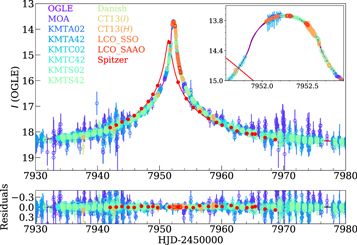
Figure 2. Ground-based and Spitzer data and best-fit model light curves of event OGLE-2017-BLG-1254 for the (0, +) model. The symbols are similar to those in Figure 1.(The data used to create this figure are available.)
Download figure:
Standard image High-resolution imageThe Spitzer observations were part of a large program to measure the Galactic distribution of planets in different stellar environments (Calchi Novati et al. 2015a; Zhu et al. 2017). The detailed protocols and strategies for the Spitzer observations are discussed in Yee et al. (2015a). Specifically, the two events were observed by the Spitzer satellite because they were both high-magnification events, which are more sensitive to planets (Griest & Safizadeh 1998). The Spitzer observations were taken using the 3.6 μm channel (L−band) of the IRAC camera.
Ground-based surveys included the Optical Gravitational Lensing Experiment (OGLE, Udalski et al. 2015a), the Microlensing Observations in Astrophysics (MOA, Sumi et al. 2016), and the Korea Microlensing Telescope Network (KMTNet, Kim et al. 2016). OGLE is in its fourth phase (OGLE-IV), and the observations are carried out using its 1.3 m Warsaw Telescope equipped with a 1.4 deg2 field-of-view (FOV) mosaic CCD camera at the Las Campanas Observatory in Chile. The MOA group conducts a high-cadence survey toward the Galactic bulge using its 1.8 m telescope equipped with a 2.2 deg2 FOV camera at the Mt. John University Observatory in New Zealand. KMTNet consists of three 1.6 m telescopes, equipped with 4 deg2 FOV cameras at the Cerro Tololo Inter-American Observatory (CTIO) in Chile (KMTC), the South African Astronomical Observatory (SAAO) in South Africa (KMTS), and the Siding Spring Observatory (SSO) in Australia (KMTA). The majority of observations were taken in the I band for the OGLE and KMTNet groups, and the MOA-Red filter (which is similar to the sum of the standard Cousins R- and I-band filters) for the MOA group, with occasional observations taken in the V band.
The aim of the ground-based follow-up observations was to detect and characterize any planetary signatures with dense observations, which are crucial if an event is not heavily monitored by ground-based surveys (e.g., OGLE-2017-BLG-1161) or the ground-based surveys could not observe due to weather (e.g., OGLE-2016-BLG-1045 Shin et al. 2018). The follow-up teams included the Las Cumbres Observatory (LCO) global network, the Microlensing Follow-up Network (μFUN, Gould et al. 2010), and Microlensing Network for the Detection of Small Terrestrial Exoplanets (MiNDSTEp, Dominik et al. 2010). The LCO global network provided observations from its 1.0 m telescopes located at CTIO, SAAO, and SSO, with the SDSS-i' filter. The μFUN team followed the events using the 1.3 m SMARTS telescope at CTIO (CT13) with the V/I/H bands (DePoy et al. 2003), the 0.4 m telescope at Auckland Observatory (AO) using a number 12 Wratten filter (which is similar to R-band), and the 0.36 m telescope at Kumeu Observatory (Kumeu) in Auckland. The MiNDSTEp team monitored the events using the Danish 1.54 m telescope sited at ESO's La Silla observatory in Chile, with a non-standard filter.
We provide detailed descriptions of the observations for OGLE-2017-BLG-1161 and OGLE-2017-BLG-1254 in the next section.
2.1. OGLE-2017-BLG-1161
OGLE-2017-BLG-1161 was discovered by the OGLE collaboration on 2017 June 20. With equatorial coordinates (α, δ)J2000 = (17:41:12.65, −26:44:28.1) and Galactic coordinates (ℓ, b) = (1.36, 1.98), it lies in OGLE field BLG652, monitored by OGLE with a cadence of 0.5–1 observations per night (Udalski et al. 2015a). This event was located in the gap of two CCD chips of KMTNet BLG15 field, thus the follow-up observations were important supplements to the sparse observations from the ground-based surveys. The I/H-band observations from CT13 intensively covered the falling side of the peak, and its H-band data calibrated to VVV H-band data (Saito et al. 2012) were also used to derive the color of the source because this event suffered from very high extinction (AI ∼ 4.5; See Section 4). In addition, OGLE-2017-BLG-1161 was also densely observed by the LCO network, the 0.4 m telescope at Auckland Observatory (AO), and the 0.36 m telescope at Kumeu Observatory (Kumeu). OGLE-2017-BLG-1161 was selected as a "secret" Spitzer target on 2017 June 25 (UT 16:00) because the newest OGLE point (HJD = 2457932.78) indicated a significant rise (consistent with a high-magnification event) and the event was predicted to peaked within 1 day, and it was formally announced as a Spitzer target on 2017 June 28. The Spitzer observations began on 2017 June 30 and ended on 2017 July 13 with 16 data points in total.
2.2. OGLE-2017-BLG-1254
OGLE-2017-BLG-1254 was first alerted by the OGLE collaboration on 2017 July 2. The event was located at equatorial coordinates (α, δ)J2000 = (17:57:23.56, −27:13:13.3), corresponding to Galactic coordinates (ℓ, b) = (2.80, −1.36). It therefore lies in OGLE field BLG645, which has a cadence less than 0.5 observations per night (Udalski et al. 2015a). This event was also identified by the MOA group as MOA-2017-BLG-373 ∼12.2 days later (Bond et al. 2001), and recognized by KMTNet's event-finding algorithm as KMT-2017-BLG-0374 (Kim et al. 2018). The KMTNet group observed this event in its two slightly offset fields BLG02 and BLG42, with combined cadence of Γ = 4 hr−1. The LCO, μFUN, and MiNDSTEp follow-up teams also observed this event. The dense observations during the peak by LCO and MiNDSTEp were important to constrain the finite-source effects. The H-band observations taken by CT13 were important for characterizing the source star because this event suffered from very high extinction (AI ∼ 4.2; see Section 4). OGLE-2017-BLG-1254 was chosen as a "secret" Spitzer target on 2017 July 2 (UT 20:48) because (1) the model predicted that the event could be a high-magnification event; and (2) KMTNet has a high cadence of Γ = 4 hr−1. It was "subjectively" selected on July 6 and became "objective" on July 17 (see Yee et al. 2015a). The Spitzer observations began on 2017 July 7 and ended on 2017 August 3 with a cadence of ∼1 observation per day.
2.3. Data Reductions
The photometry of OGLE, MOA, KMTNet, LCO, AO, Kumeu, and Danish data was extracted using custom implementations of the difference image analysis technique (Alard & Lupton 1998): Wozniak (2000) (OGLE), Bond et al. (2001) (MOA), Albrow et al. (2009) (KMTNet, LCO, AO, and Kumeu), and Bramich (2008) (Danish). In addition, the CT13 data were reduced by DoPHOT (Schechter et al. 1993). The Spitzer data were reduced using the algorithm developed by Calchi Novati et al. (2015b) for crowded-field photometry.
3. Light-curve Analysis
3.1. Ground-based Data Only
For each event, we model the ground-based data using four parameters for the magnification, A(t). These include three Paczyński parameters (t0, u0, tE; Paczyński 1986) to describe the light curve produced by a single-lens with a point-source: the time of the maximum magnification as seen from Earth t0, the impact parameter u0 (in units of the angular Einstein radius θE), and the Einstein radius crossing time tE. In addition, the source size normalized by the angular Einstein radius ρ is needed to incorporate finite-source effects. The flux, f(t), calculated from the model is

where fs represents the flux of the source star being lensed, and fb is any blended flux that is not lensed. The two linear parameters, fs and fb, are different for each observatory and each filter. In addition, we adopt the linear limb-darkening law to consider the brightness profile of the source star (An et al. 2002)

where  is the mean surface brightness of the source, θ is the angle between the normal to the surface of the source and the line of sight, and Γλ is the limb-darkening coefficient at wavelength λ. We employ the Markov chain Monte Carlo (MCMC) χ2 minimization using the emcee ensemble sampler (Foreman-Mackey et al. 2013) to find the best-fit parameters and their uncertainties.
3.2. Satellite Parallax
We measure the microlens parallax from the light-curve modeling:

where Δt0 is the difference in event peak time t0 and Δu0 is the difference in impact parameter u0 as seen from the Spitzer satellite and Earth, and D⊥ is the projected separation between the Spitzer satellite and Earth at the time of the event. Generally, only the absolute value of u0 can be measured from the modeling, thus the satellite parallax measurements usually suffer from a fourfold degeneracy (Refsdal 1966; Gould 1994). We specify the four solutions as (+, +), (+, −), (−, −), and (−, +) using the sign convention described in Zhu et al. (2015). Briefly, the first and second signs in each parenthesis indicate the signs of u0,⊕ and u0,Spitzer, respectively. In addition, the Spitzer observations only cover the falling part of OGLE-2017-BLG-1161, which leads to large uncertainty of πE. Thus, we include a color–color constraint on the Spitzer source flux fs,Spitzer to improve the parallax measurement (e.g., Calchi Novati et al. 2015a). This constraint adds a  into the total χ2 (see Equation (2) in Shin et al. 2017 for the form of the
  ).
).
3.3. OGLE-2017-BLG-1161
Using the intrinsic color of the source star (see Section 4.1) and the color–temperature relation of Houdashelt et al. (2000), we estimate the effective temperature of the source to be Teff ≈ 4450 K. Applying ATLAS models and assuming a surface gravity of  = 2.5, a metallicity of [M/H] = 0.0, and a microturbulence parameter of 1 km s−1, we obtain the linear limb-darkening coefficients uI = 0.60 for the I band, uV = 0.81 for the V band, uR = 0.71 for the R band, uH = 0.39 for the H band, and uL = 0.24 for the L band (Claret & Bloemen 2011). We then employ the transformation formula in An et al. (2002) and Fields et al. (2003), yielding the corresponding limb-darkening coefficients ΓI = 0.50, ΓV = 0.74, ΓR = 0.62, ΓH = 0.30, and ΓL = 0.18. In the light-curve modeling, we use ΓI for OGLE, LCO, CT13 I−band, and Kumeu data, ΓAO = (ΓV+ΓR)/2 = 0.68 for AO data, ΓH for CT13 H−band data, and ΓL for Spitzer data.
To derive the color–color constraint on the Spitzer source flux fs,Spitzer, we extract the Spitzer photometry of red giant bulge stars (4.0 < IOGLE−HVVV < 5.5; 17.5 < IOGLE < 20.0) and fit for the two parameters in the equation60

where Xp = 4.65 is a pivot parameter chosen to minimize the covariance between the parameters. We then obtain c0 = 4.47 ± 0.01, c1 = 1.28 ± 0.03 (see Figure 3 for the fit of the color–color relation). This, when combined with (IOGLE−HVVV)S = 4.71 ± 0.01 (see Section 4.1), yields (IOGLE−LSpitzer)S = 4.55 ± 0.02. We employ this constraint on the light-curve modeling.

Figure 3. In each panel, the blue circles with error bars represent the Spitzer, OGLE, and VVV photometry of the red giants, and the red dots represent the positions of the source star. The black line is the best-fit linear model.
Download figure:
Standard image High-resolution imageTable 1 shows the best-fit parameters and their 1σ uncertainties for the fourfold degenerate solutions (Δχ2 < 0.16). The best-fit model curves for the (−, +) solution are shown in Figure 1. For all the fourfold degenerate solutions, the east component πE,E of the microlens parallax vector is ∼0.038 ± 0.06, while the north component πE,N is consistent with 0 at the ∼2σ level.
Table 1. Best-fit Parameters for OGLE-2017-BLG-1161 and OGLE-2017-BLG-1254 and Their 68% Uncertainty Range from the MCMC
| Event | OGLE-2017-BLG-1161 | OGLE-2017-BLG-1254 | ||||
|---|---|---|---|---|---|---|
| Solution | (+, +) | (+, −) | (−, −) | (−, +) | (0, +) | (0, −) |
| t0,⊕ −2450000(d) | 7933.548(2) | 7933.548(2) | 7933.548(2) | 7933.548(2) | 7952.2519(4) | 7952.2518(4) |
| u0,⊕ | 0.0214(8) | 0.0214(9) | −0.0214(9) | −0.0214(9) | 0.0003(10) | −0.0003(9) |
| tE | 9.5(3) | 9.5(3) | 9.5(3) | 9.4(3) | 15.43(6) | 15.42(7) |
| ρ | 0.0464(15) | 0.0465(15) | 0.0467(15) | 0.0466(16) | 0.0251(1) | 0.0251(1) |
| πE,N | −0.000(23) | −0.034(21) | −0.000(22) | 0.037(22) | 0.0203(7) | −0.0174(7) |
| πE,E | 0.039(7) | 0.038(5) | 0.038(5) | 0.037(6) | 0.0368(4) | 0.0384(5) |
| πE | 0.039(9) | 0.051(17) | 0.038(8) | 0.052(16) | 0.0420(7) | 0.0421(7) |
| Is,OGLE | 18.71(3) | 18.70(3) | 18.70(3) | 18.70(3) | 18.53(1) | 18.53(1) |
| Ib,OGLE | 18.71(3) | 18.72(3) | 18.72(3) | 18.72(3) | 21.32(6) | 21.32(6) |
| χ2penalty | 0.00 | 0.02 | 0.01 | 0.02 | ⋯ | ⋯ |
| χ2/dof | 618.41/617 | 618.35/617 | 618.25/617 | 618.30/617 | 8254.78/8256 | 8254.69/8256 |
Download table as: ASCIITypeset image
3.4. OGLE-2017-BLG-1254
Applying the same procedure as in Section 3.3, we obtain the corresponding limb-darkening coefficients ΓI = 0.45, ΓR = 0.55, ΓH = 0.26, and ΓL = 0.16. In the light-curve modeling, we use ΓI for OGLE, KMTNet, LCO, CT13 I−band, and Danish data, ΓMOA = (ΓI+ΓR)/2 = 0.50 for MOA data, ΓH for CT13 H-band data, and ΓL for Spitzer data. We find that the impact parameter u0,⊕ ≃ 0, so the four degenerate solutions reduce to two solutions [(0, +), (0, −)], with Δχ2 = 0.09. However, this degeneracy has no effect on the mass and distance measurement for the lens (Gould & Yee 2012; Shin et al. 2018). The best-fit model curves for (0, +) are shown in Figure 2, and the best-fit parameters for the two degenerate solutions are shown in Table 1.
For this event the Spitzer light curve precisely constrains the microlens parallax without the need of a color–color constraint on LSpitzer. Nevertheless, we derive the IHL color–color relation using red giants (3.6 < IOGLE−HVVV < 5.0; 17.0 < IOGLE < 19.5) for validation of the color–color method. The relation and the (IOGLE−HVVV)S color in Section 4.2 suggest (IOGLE−LSpitzer)S = 3.82 ± 0.03, which is in excellent agreement with the color measured from the model of (IOGLE−LSpitzer)S = 3.82 ± 0.01.
3.5. Effect of the Color–Color Constraint
A method to check the Spitzer photometry is to compare the parallax constraint with and without color–color constraints.
To investigate the effect of the color–color constraint, we fit the parallax for the two events both with and without imposing the constraint. We plot the likelihood distributions for  derived from the MCMC chain in Figures 4 and 5.
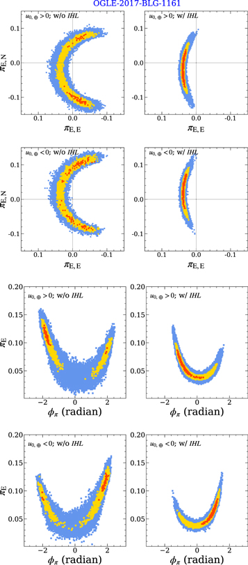
Figure 4. Likelihood distributions for πE,E vs. πE,N (upper four panels) and ϕπ vs. πE (lower four panels) for OGLE-2017-BLG-1161, respectively. Here  . The left panels show the distributions without the IHL color–color relation, and the right panels show the distributions with the relation. In each panel, red, yellow, and blue show likelihood ratios
 ![$[-2{\rm{\Delta }}\mathrm{ln}{ \mathcal L }/{{ \mathcal L }}_{\max }]\lt (1,4,\infty )$](https://content.cld.iop.org/journals/0004-637X/891/1/3/revision1/apjab6ff8ieqn10.gif) , respectively.
, respectively.
Download figure:
Standard image High-resolution image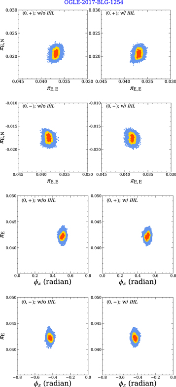
Figure 5. Likelihood distributions for πE,E vs. πE,N (upper four panels) and ϕπ vs. πE (lower four panels) for OGLE-2017-BLG-1254, respectively. The symbols have the same meanings as those in Figure 4.
Download figure:
Standard image High-resolution imageFor OGLE-2017-BLG-1161, we find that the most likely solutions without the color–color constraint are consistent with the solutions with the color–color constraint, and the color–color constraint reduces the uncertainty of the parallax measurements. The plots show that even though there is a large uncertainty in the direction of the parallax vector, its magnitude is well-constrained, even without the color–color constraint. The arc-like form of the parallax contours arises because the Spitzer measurements began after the peak of the event and each contributed a series of oscillating circular constraints (Gould 2019).
For OGLE-2017-BLG-1254, the color–color constraint has basically no effect on the derived parallax, which is expected since the Spitzer observations cover the peak of the light curve.
4. Physical Parameters: Two Low-mass Stars in the Galactic Bulge
4.1. OGLE-2017-BLG-1161L
To derive the angular Einstein radius θE for the lens by Equation (3), we estimate the angular radius θ* of the source by locating it on a color–magnitude diagram (Yoo et al. 2004). We construct an I−H versus I color–magnitude diagram by cross-matching the OGLE-IV I-band and the VVV H-band stars within a 2' × 2' square centered on the event (See Figure 6). We estimate the red giant clump to be (I−H, I)cl = (4.59 ± 0.02, 18.90 ± 0.03) and find that the position of the source is (I−H, I)S = (4.71 ± 0.01, 18.70 ± 0.03) from OGLE I−band data and CT13 H−band data aligned to the VVV magnitudes. From Nataf et al. (2016), we find that the intrinsic color and dereddened magnitude of the red clump are (I−H, I)cl,0 = (1.30, 14.39). Thus, the intrinsic color and dereddened brightness of the source are (I−H, I)S,0 = (1.42 ± 0.03, 14.19 ± 0.04). These values suggest the source is a K-type giant star (Bessell & Brett 1988). Using the color/surface-brightness relation of Adams et al. (2018), we obtain

We derive the angular Einstein radius and the geocentric lens-source relative proper motion


Using Equation (1), we measure the lens mass,


The lens-source relative parallax for the two cases is


which are very small compared to the source parallax πS ≃ 0.12 (Nataf et al. 2016). Thus, the distance between the lens and the source is determined much more precisely than the distance to the lens or the source separately. We measure the lens-source distance,


where we adopt the source distance DS = 8.0 ± 0.8 kpc using the Galactic model of Zhu et al. (2017). Because the lens-source distance is ≲1 kpc and the source is almost certainly a bulge red-clump star, the lens should be an M/K dwarf in the Galactic bulge. We list the derived source star properties in Table 2 and the physical parameters of all the fourfold degenerate solutions in Table 3. In addition, we predict the lens apparent magnitude in the I and H bands using the MIST isochrones,61 which are shown in Table 3.
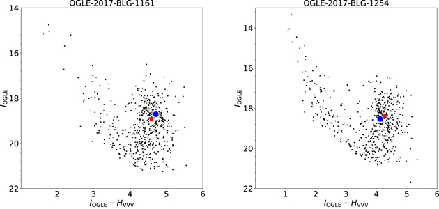
Figure 6. OGLE-VVV color–magnitude diagrams of a 2' × 2' square centered on OGLE-2017-BLG-1161 (left panel) and OGLE-2017-BLG-1254 (right panel). The red asterisks show the centroid of the red clump. The blue dots indicate the position of the source.
Download figure:
Standard image High-resolution imageTable 2. Derived Source Star Properties for OGLE-2017-BLG-1161 and OGLE-2017-BLG-1254
| Parameters | Units | Value | |
|---|---|---|---|
| OGLE-2017-BLG-1161 | OGLE-2017-BLG-1254 | ||
| AI | (mag) | ∼4.5 | ∼4.2 |
| IS | (mag) | 18.70 ± 0.03 | 18.53 ± 0.01 |
| HS | (mag) | 13.99 ± 0.03 | 14.41 ± 0.01 |
| (I−H)S | 4.71 ± 0.01 | 4.12 ± 0.02 | |
| (I−L)S | 4.55 ± 0.02 | 3.81 ± 0.02 | |
| IS,0 | (mag) | 14.19 ± 0.04 | 14.51 ± 0.03 |
| HS,0 | (mag) | 12.77 ± 0.04 | 13.37 ± 0.03 |
| (I−H)S,0 | 1.42 ± 0.03 | 1.14 ± 0.03 | |
| θ* | (μas) | 7.4 ± 0.04 | 5.2 ± 0.03 |
Download table as: ASCIITypeset image
Table 3. Physical Parameters and Predicted Lens I- and H-band Brightness for OGLE-2017-BLG-1161 and OGLE-2017-BLG-1254
| Event | OGLE-2017-BLG-1161 | OGLE-2017-BLG-1254 | |||
|---|---|---|---|---|---|
| Solution | (+, +) | (+, −) | (−, −) | (−, +) | (0, +) and (0, −) |
| θE (mas) | 0.159 ± 0.009 | 0.159 ± 0.009 | 0.159 ± 0.009 | 0.159 ± 0.009 | 0.207 ± 0.008 |
| ML (M⊙) |

|

|

|

|
0.60 ± 0.03 |
| DLS (kpc) | 0.40 ± 0.12 | 0.53 ± 0.19 | 0.40 ± 0.12 | 0.53 ± 0.19 | 0.53 ± 0.11 |
| μrel (mas yr−1) | 6.11 ± 0.39 | 6.11 ± 0.39 | 6.11 ± 0.39 | 6.11 ± 0.39 | 4.90 ± 0.20 |
| IL (mag) | 26.5 ± 0.9 | 27.5 ± 0.9 | 26.5 ± 0.9 | 27.5 ± 0.9 | 25.1 ± 0.4 |
| HL (mag) | 21.0 ± 0.6 | 21.8 ± 0.6 | 21.0 ± 0.6 | 21.8 ± 0.6 | 20.4 ± 0.2 |
Download table as: ASCIITypeset image
4.2. OGLE-2017-BLG-1254L
We construct an I−H versus I color–magnitude diagram via the OGLE-IV I-band and the VVV H-band stars within a 2' × 2' square centered on the event (See Figure 6). We measure the centroid of the red giant clump (I−H, I)cl = (4.28 ± 0.02, 18.39 ± 0.03) and the position of the source (I−H, I)S = (4.12 ± 0.02, 18.53 ± 0.01). From Nataf et al. (2016), we find that the intrinsic color and dereddened magnitude of the red clump are (I−H, I)cl,0 = (1.30, 14.35), from which we derive the intrinsic color and dereddened brightness of the source as (I−H, I)S,0 = (1.14 ± 0.03, 14.51 ± 0.03). Thus, the source is a G-type giant star (Bessell & Brett 1988). Applying the color/surface-brightness relation of Adams et al. (2018), we obtain


where we also adopt the source distance DS = 7.8 ± 0.8 kpc using the Galactic model of Zhu et al. (2017). Thus, the lens is probably a K dwarf in the Galactic bulge. We list the derived source star properties in Table 2 and the physical parameters of OGLE-2017-BLG-1254 in Table 3.
5. Discussion and Conclusion
We have reported an analysis of two microlensing events, OGLE-2017-BLG-1161 and OGLE-2017-BLG-1254, each of which displays both finite-source effects detected by the ground-based data and a microlens parallax measured by the joint analysis of the ground-based data and the Spitzer data. Including these two events, the Spitzer microlensing program has measured the mass and distance for eight isolated objects from 2015 to 2017, yielding an estimate of the apparent detection frequency ∼8/328 = 2.4%.62 This apparent frequency agrees with the theoretical frequency ∼3.3% (Zhu et al. 2016) within 1σ for Poisson statistics. The theoretical frequency assumes that the probability of detecting the finite-source effects in single-lens events is the same for ground and Spitzer observations, but the Spitzer data only detected finite-source effects for two events63 (OGLE-2015-BLG-0763 Zhu et al. 2016, OGLE-2015-BLG-1482 Chung et al. 2017), with a degeneracy in ρ. This is because the Spitzer observations only have a Γ ∼ day−1 cadence and require a 3–10 day turnaround time after selection of the event, leading to the loss of finite-source effect detection from Spitzer observations.
The probability of finite-source effects occurring in a single-lens event is

This, when combined with the microlensing rate Γμlens ∝ nμrelθE (n is the number density), yields the finite-source event rate (Gould & Yee 2012; Shvartzvald et al. 2019)

We apply the Galactic model described in Zhu et al. (2017) and estimate the probability density distribution of finite-source events based on n × μrel. We average the distributions in the direction of the eight Spitzer finite-source events and assume the source distances are 8.3 kpc for all the events (following Zhu et al. 2017). For events with two degenerate solutions, both solutions are included at half the weight. Figure 7 compares the resulting probability densities for different masses and distances with the eight Spitzer finite-source events. Figures 8 and 9 compare the cumulative distributions of the lens distance and lens mass, respectively. In this comparison, we do not take into account the Spitzer detection efficiency, and possible selection or publication biases. Such a detailed analysis is beyond the scope of this paper and will be done in a future complete statistical analysis of the Spitzer campaigns.
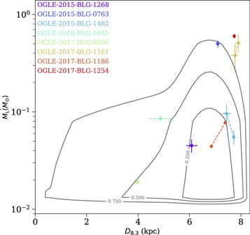
Figure 7. Bayesian probability density distributions from the Galactic model of Zhu et al. (2017) compared to the eight published Spitzer finite-source events. We fix the source distance to 8.3 kpc and then derive the lens distance D8.3 for all the events. The predicted mass distribution is derived from the initial mass function of Kroupa (2001). The dots with different colors represent different events. The two dots connected by dashed lines represent the two degenerate solutions of one event. The gray lines represent equal probability density. The values on the contours indicate the total probability inside the contours predicted by the Galactic model, and the total probability is normalized to unity.
Download figure:
Standard image High-resolution image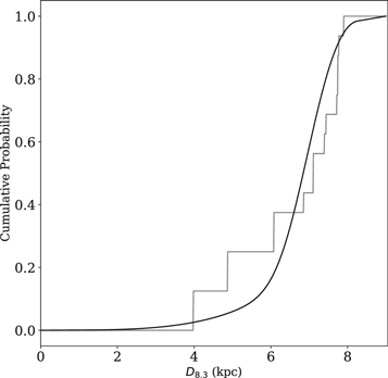
Figure 8. Cumulative distribution of the lens distance from the Galactic model of Zhu et al. (2017) and the eight published Spitzer finite-source events. We fix the source distance of 8.3 kpc and then derive the lens distance D8.3 for all the events. The black line represents the distribution predicted by the Galactic model, and the gray lines represent the distribution calculated from the eight events. The observed distribution is consistent with the Galactic model with a Kolmogorov–Smirnov probability of 86.8%.
Download figure:
Standard image High-resolution image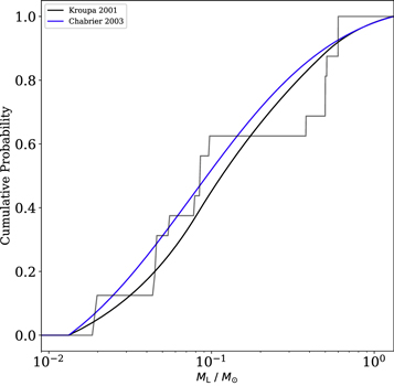
Figure 9. Cumulative distribution of the lens mass from the initial mass function and the eight published Spitzer finite-source events. The black line represents the distribution predicted by the initial mass function of Kroupa (2001) and the blue line represents the distribution calculated from Chabrier (2003). The observed distribution is consistent with the initial mass functions of Kroupa (2001) and Chabrier (2003), with Kolmogorov–Smirnov probabilities of 84.9% and 72.3%, respectively.
Download figure:
Standard image High-resolution image
The observed Spitzer sample agrees with expectations from the Galactic model. The distance distribution of the eight events is consistent with the Galactic model of Zhu et al. (2017), with a Kolmogorov–Smirnov probability of 86.8%, and the mass distribution is consistent with the initial mass function of Kroupa (2001) and Chabrier (2003), with Kolmogorov–Smirnov probabilities of 84.9% and 72.3%, respectively. Both the Galactic model and the eight Spitzer events show that the finite-source effects have strong bias toward objects in the Galactic bulge. This is primarily because the stellar number density in the Galactic bulge is significantly higher than that of the Galactic disk, while the lens-source relative proper motions of disk lenses are only slightly higher on average (see Figures 1 and 2 of Zhu et al. 2017).
Shan et al. (2019) compared 13 well-characterized Spitzer systems (10 binary/planetary lenses and 3 single lenses) with Bayesian predictions from Galactic models and found that they are in excellent agreement. Our preliminary comparisons of eight Spitzer single lenses also suggests good agreement with the expectations from the Galactic model. Assuming the empirical rate from 2015 to 2017 season, we expect another 5–10 detections of finite-source events in 2018 and 2019 Spitzer microlensing campaigns, and thus future statistical analyses of all Spitzer finite-source events will potentially allow a study of specific stellar populations and test the Galactic model.
Koshimoto & Bennett (2019) argued that the point-lens sample of 50 events in Zhu et al. (2017) is not consistent with the Galactic model they adopted. Gould et al. (2019) showed that the systematic errors in the Spitzer photometry for the microlensing event KMT-2018-BLG-0029 may be caused by the bright stars near the target and the rotation of the telescope with respect to the sky between images. For our events, the two sources are both red giants, so the influence of stars near the targets is weak. In addition, as discussed in Section 3.5, the parallax measurements with and without color–color constraints are basically the same. Thus, the source flux measured by Spitzer photometry and the color–color relation are basically the same, which shows that the Spitzer photometry for these two events is correct.
W.Z., W.T., S.-S.L., and S.M. acknowledge support by the National Science Foundation of China (grants No. 11821303 and 11761131004). This work is based (in part) on observations made with the Spitzer Space Telescope, which is operated by the Jet Propulsion Laboratory, California Institute of Technology under a contract with NASA. Support for this work was provided by NASA through an award issued by JPL/Caltech. The OGLE has received funding from the National Science Centre, Poland, grant MAESTRO 2014/14/A/ST9/00121 to A.U. This research has made use of the KMTNet system operated by the Korea Astronomy and Space Science Institute (KASI) and the data were obtained at three host sites of CTIO in Chile, SAAO in South Africa, and SSO in Australia. The MOA project is supported by JSPS KAKENHI grants No. JSPS24253004, JSPS26247023, JSPS23340064, JSPS15H00781, JP16H06287, and JP17H02871. The research has made use of data obtained at the Danish 1.54 m telescope at ESO's La Silla Observatory. CITEUC is funded by National Funds through FCT—Foundation for Science and Technology (project: UID/Multi/00611/2013) and FEDER—European Regional Development Fund through COMPETE 2020—Operational Programme Competitiveness and Internationalization (project: POCI-01-0145-FEDER-006922). Work by A.G. was supported by AST-1516842 and by JPL grant 1500811. A.G. received support from the European Research Council under the European Unions Seventh Framework Programme (FP 7) ERC grant Agreement No. [321035]. Wei Zhu was supported by the Beatrice and Vincent Tremaine Fellowship at CITA. Work by C.H. was supported by the grant (2017R1A4A1015178) of the National Research Foundation of Korea. Y.T. acknowledges the support of DFG priority program SPP 1992 "Exploring the Diversity of Extrasolar Planets" (WA 1047/11-1). L.M. acknowledges support from the Italian Minister of Instruction, University and Research (MIUR) through the FFABR 2017 fund.
Footnotes
- 58
OGLE-2015-BLG-1482 has two possible solutions, with M = 55 ± 9 MJ or M = 96 ± 23 MJ.
- 59
OGLE-2017-BLG-1186 has two possible solutions, with M = 45 ± 1 MJ or M = 73 ± 2 MJ.
- 60
The Spitzer L-band in this paper is in instrumental magnitude.
- 61
- 62
Spitzer observed 524 events from 2015 to 2017, but only 328 events are single-lens events with a clear Spitzer signal.
- 63
For OGLE-2017-BLG-1186, the best-fit Spitzer light curve also shows finite-source effects, but the daily Spitzer data are insufficient for the detection.