


Abstract
We present a two-epoch Hubble Space Telescope study of NGC 2071 IR highlighting HOPS 361-C, a protostar producing an arced 0.2 parsec-scale jet. The proper motions for the brightest knots decrease from 350 to 100 km s−1 with increasing distance from the source. The [Fe ii] and Paβ emission line intensity ratio gives a velocity jump through each knot of 40–50 km s−1. A new [O i] 63 μm spectrum, taken with the German REciever for Astronomy at Terahertz frequencies instrument aboard Stratospheric Observatory for Infrared Astronomy, shows a low line-of-sight velocity indicative of high jet inclination. Proper motions and jump velocities then estimate 3D flow speed for knots. Subsequently, we model knot positions and speeds with a precessing jet that decelerates. The measurements are matched with a precession period of 1000–3000 yr and half opening angle of 15°. The [Fe ii] 1.26-to-1.64 μm line intensity ratio determines visual extinction to each knot from 5 to 30 mag. Relative to ∼14 mag of extinction through the cloud from C18O emission maps, the jet is embedded at a 1/5–4/5 fractional cloud depth. Our model suggests the jet is dissipated over a 0.2 pc arc. This short distance may result from the jet sweeping through a wide angle, allowing the cloud time to fill cavities opened by the jet. Precessing jets contrast with nearly unidirectional protostellar jets that puncture host clouds and can propagate significantly farther.
Export citation and abstract BibTeX RIS

Original content from this work may be used under the terms of the Creative Commons Attribution 4.0 licence. Any further distribution of this work must maintain attribution to the author(s) and the title of the work, journal citation and DOI.
1. Introduction
NGC 2071 is a region of embedded star formation in the Orion B molecular cloud complex and is rich in intermediate-mass protostars and protostellar jets. The setting is ideal for investigation of interactions between outflows and the host molecular cloud (Bally 1982; Wootten et al. 1984; Bally 2016; Lee 2020). At IR wavelengths, the northern region is dubbed NGC 2071 IR. It contains bright protostars like HOPS 361-C (IRS 3) and HOPS 361-A (IRS 1; Walther & Geballe 2019), both of which feature prominent jets traced in molecular hydrogen emission (Eislöffel 2000). HOPS 361-A, one of the brightest sources in NGC 2071 IR, has a distance of 430.4 pc using Gaia observations (Tobin et al. 2020). The region and its protostars were recently studied at high-angular resolution with the Atacama Large Millimeter/submillimeter Array (ALMA) and the Very Large Array (VLA) by Cheng et al. (2022).
HOPS 361-C is the proposed driving source for the largest NE–SW outflow bright in molecular hydrogen. The outflow features large  arcs on both sides of the HOPS 361 region (Eislöffel 2000). HOPS 361-C is a class 0 protostar (Tobin et al. 2020), although it is borderline with class I according to its bolometric temperature of 69 K (Furlan et al. 2016). A Keplerian molecular disk is resolved with ALMA in SO 65–54, with an outer disk radius of ∼150 au and position angle of ∼130° approximately perpendicular to a high-velocity CO jet (Cheng et al. 2022).
Misaligned segments and wiggles in the outflow tracer, CO J = 2–1, led Cheng et al. (2022) to propose that the molecular jet is produced by a young stellar object with a precessing disk. A jet that precesses due to tidal interactions in a binary system may experience wide variations in direction. These variations occur when the jet axis is tilted or misaligned with respect to the direction normal to the binary's orbital plane (Terquem et al. 1999; Masciadri & Raga 2002).
Variations in jet direction can also affect stellar feedback and ensuing star formation. If the jet remains at a fixed angle, then a single cavity is cleared within a molecular cloud (Cunningham et al. 2009a). In contrast, arced jets can affect a larger volume of the undisturbed cloud (Hartigan et al. 2001) or be dissipated locally (Fendt & Yardimci 2022). By comparing properties of wide, arced jets with those that exhibit small opening angles, we can constrain how the jet propagates into the ambient molecular cloud, an important step toward quantifying the reach of feedback.
Bright gaseous knots trace shocks in protostellar jets and outflows, and their positions along a jet can wiggle (e.g., Raga et al. 2002). These wiggles have been attributed to variations in jet velocity caused by orbital motion within a binary system or by variations in jet orientation due to precession (Masciadri & Raga 2002; Anglada et al. 2007; Erkal et al. 2021). If both a jet and counter-jet are observed, the two scenarios can be differentiated via examination of the symmetry pattern of the jet trajectory. Mirror-symmetry is expected in the case of binary orbital motion; an S-shaped morphology is expected in the case of precession. These two types of models can be applied to the jet and knot positions, directly relating periodicity in the knot positions to the binary period or precession period (e.g., Raga et al. 2002). Most prior work focuses on molecular jets with small wiggles and opening angles (i.e., the angular width of the jet) of <10°; these are usually interpreted in terms of binary motion (Gueth et al. 1996; Zinnecker et al. 1998; Woitas et al. 2002; Chandler et al. 2005; Sahai et al. 2005; Ybarra et al. 2006; Seale & Looney 2008; Phillips & Pérez-Grana 2009; Lee et al. 2010, 2015; Whelan et al. 2010; Agra-Amboage et al. 2011; Noriega-Crespo et al. 2011, 2020; Estalella et al. 2012; Fernández-López et al. 2013; Velázquez et al. 2014; Kwon et al. 2015; Beltrán et al. 2016; Moraghan et al. 2016; Choi et al. 2017; Louvet et al. 2018; Hara et al. 2021; Jhan & Lee 2021; Murphy et al. 2021; Massi et al. 2022, 2023).
Some jets exhibit a visible S-shape but have a narrow opening angle of 8°, like the L1157 molecular outflow and jet (Podio et al. 2016). The outflow from HOD07 1 in Monoceros R2 (Hodapp 2007), from IRAS 4A2 in NGC 1333 (Hodapp et al. 2005; Jørgensen et al. 2006; Chuang et al. 2021), the jet in Barnard 1 denoted B1c (Matthews et al. 2006), and the collimated outflows surveyed in the Cores to Disks Spitzer Legacy program (Seale & Looney 2008) all show an S-shaped morphology and are likely to have wider opening angles. S-shaped jets and jets that appear to have a wide opening angle are often interpreted in terms of only precession of the binary orbit (Hodapp et al. 2005; Jørgensen et al. 2006; Matthews et al. 2006; Podio et al. 2016; Lee 2020; Chuang et al. 2021). However, Cunningham et al. (2009b) proposed that the HW2 protostellar source in the Cepheus A region precessed due to capture of a binary partner, but this result cannot entirely rule out the binary precessing (Ferrero et al. 2022). Variations in jet direction can also be due to asymmetric infall from the envelope or tidal torque from the envelope resulting in disk precession (Hirano & Machida 2019). The massive protostar IRAS 20126 + 4104 has a precessing jet with the widest known opening angle of 40°, but CO imaging did not distinguish between possible interpretations (Shepherd et al. 2000).
Subarcsecond resolution and multiepoch observations are required to study the morphology and motion of bright knots along a protostellar jet (Bally 1982; Reiter et al. 2017; Hartigan et al. 2019; López et al. 2022). Near-infrared (NIR) emission lines can be used to detect these knots in heavily extinguished regions (e.g., Erkal et al. 2021). Shocks throughout a jet consist of sharp, discontinuous jumps in density and velocity, called jump or J-type, and continuous versions or C-type. To separate emission from dust and from shocks, the forbidden and atomic spectral lines, like [Fe ii] and Paβ respectively, are used to determine extinction and to study hot, ionized, and shocked gas in protostellar jets (e.g., Erkal et al. 2021; Reiter et al. 2017).
We focus on HOPS 361-C, which has a clear and distinct string of knots tracing an arced jet with a wide opening angle. In Section 2, we present new Hubble Space Telescope (HST) observations of NGC 2071 IR in [Fe ii] and Paβ and NIR HST images from an earlier epoch. The knots of emission are detected, presumed from J-type shocks associated with the jet. We also present a new [O i] spectrum using the German REciever for Astronomy at Terahertz frequencies (GREAT) instrument on the Stratospheric Observatory for Infrared Astronomy (SOFIA), which measures the radial velocity near the base of the jet, and constrains the orientation of the outflow relative to the plane of the sky. In Section 3, we use the multiepoch data to measure knot proper motions. In Section 4, we discuss constraints on shock models and use [Fe ii] line ratios to calculate the extinction to each knot in the jet. In Section 5, we discuss models that can account for the speed and morphology of the jet originating from HOPS 361-C. The shock speeds from our spectral line images combine with the tangential speeds from proper motions to give the jet's momentum and kinetic energy injection rate into the cloud. With our model of HOPS 361-C's jet, we estimate the rate that jet material is decelerated by interacting with the molecular cloud.
2. Observations and Data Reduction
2.1. HST WFC3/IR
NGC 2071 was observed twice with HST's Wide Field Camera 3/Infrared (WFC3/IR). The first epoch is centered on NGC 2071 IR and the protostellar sources HOPS 361 (A)–(F). These images were taken on 2010 March 8 from HST General Observer (GO) proposal 11548 (Kounkel et al. 2016; Habel et al. 2021). The second epoch of images were taken between 2021 September 16 and November 3 as part of a joint HST/SOFIA GO proposal 16493. That program observed three fields to cover the entire HOPS 361-C jet, the HOPS 361-A outflow cavity, and the region surrounding these features.
The image frames were acquired with HST/WFC3 in star tracker-guided mode and using a standard 4-point dither. WFC3's field of view is 136'' × 123'' at NIR wavelengths. The images were captured using the following narrowband, NIR filters (and relevant spectral features): F126N (1.26 μm [Fe ii]), F128N (1.28 μm Paβ), F130N (1.30 μm continuum), F164N (1.64 μm [Fe ii]), F167N (1.67 μm continuum). Images are standard data products outputted by the calwf3 pipeline, retrieved from the Barbara A. Mikulski Archive for Space Telescopes (MAST) with suffix "FLT," and have details in Table 1.
Table 1. Observing Details
| Target | Observation ID | Date | Filter | Spectral Line and Wavelength | Exposure Time |
|---|---|---|---|---|---|
| (s) | |||||
| HOPS 369 | IB0L9X010 | 2010 Mar 8 | F160N | Continuum 1.60 μm | 2496 |
| HOPS361-center | IEJ707010 | 2021 Nov 1 | F126N | [Fe ii] 1.257 μm | 1797.7 |
| HOPS361-center | IEJ708010 | 2021 Nov 1 | F128N | H i Paβ 1.282 μm | 1797.7 |
| HOPS361-center | IEJ707020, IEJ708020 | 2021 Nov 1 | F130N | Continuum 1.30 μm | 597.7, 597.7 |
| HOPS361-center | IEJ701010 | 2021 Sep 16 | F164N | [Fe ii] 1.644 μm | 2396.9 |
| HOPS361-center | IEJ702010 | 2021 Sep 16 | F167N | Continuum 1.67 μm | 2396.9 |
| HOPS361-SW | IEJ705010 | 2021 Sep 30 | F164N | [Fe ii] 1.644 μm | 2396.9 |
| HOPS361-SW | IEJ706010 | 2021 Nov 1 | F167N | Continuum 1.67 μm | 2396.9 |
| HOPS361-SW | IEJ711010 | 2021 Nov 3 | F126N | [Fe ii] 1.257 μm | 1797.7 |
| HOPS361-SW | IEJ711020, IEJ712020 | 2021 Nov 3 | F130W | Continuum 1.30 μm | 597.7, 597.7 |
| HOPS361-SW | IEJ712010 | 2021 Nov 3 | F128N | H i Paβ 1.282 μm | 1797.7 |
| HOPS361-NE | IEJ703010 | 2021 Sep 27 | F164N | [Fe ii] 1.644 μm | 2396.9 |
| HOPS361-NE | IEJ704010 | 2021 Sep 29 | F167N | Continuum 1.67 μm | 2396.9 |
| HOPS361-NE | IEJ709010 | 2021 Nov 2 | F126N | [Fe ii] 1.257 μm | 1797.7 |
| HOPS361-NE | IEJ709020, IEJ710020 | 2021 Nov 2 | F130N | Continuum 1.30 μm | 597.7, 597.7 |
| HOPS361-NE | IEJ710010 | 2021 Nov 2 | F128N | H i Paβ 1.282 μm | 1797.7 |
Note. Target and observation IDs taken from MAST ordered by date of observation. Target centers (J2000 R.A., decl.) were HOPS369 at (05h47m01 606, +00d17m5888), HOPS361-Center at (05h46m58943, +00d20m4112), HOPS361-SW at (05h46m58943, +00d20m4112), HOPS361-NE at (05h47m09900, +00d23m4672).
Download table as: ASCIITypeset image
We aligned images using the Python drizzlepac package with default parameters. The images in all filters were simultaneously aligned using the TweakReg routine version 1.4.7 to give a subpixel accuracy. We estimate errors in the image shifts to be at most 0.05 pixels or ∼0 006 based on comparing centroids of stars in images at the two different epochs.
The Astrodrizzle algorithm (Hoffmann et al. 2021) version 3.3.0 was used with default parameters to resample the images to the same pixel size of 012825 × 012825 and remove defects (e.g., cosmic rays, bad pixels). The same routine was used to mosaic sets of second epoch narrowband images with the same filter. We then used the IPAC software Montage to shift, regrid, and update the World Coordinate System to the same frame size and orientation. This gave a final spatial (angular) resolution by 2D Gaussian FWHM of about 2 pixels (02565) for epoch (1) and about 3 pixels (038475) for epoch (2).
To convert e-/s to units of intensity, we used the flux density and bandwidth calibration values in the FITS file headers produced by the HST calibration pipeline (keywords PHOTFLAM and PHOTBW). The rms noise in the central frame for all images and within circular areas ranging from 1 to 15 arcsec2 (used through this work) is 1.55 ×10⁻¹⁸ erg cm−2 s−1 per pixel as measured in regions devoid of stars and nebulosity.
For the precise coalignment needed to compute proper motions, the F160W frames were separately reprocessed through with drizzlepac, Astrodrizzle, and Montage as described with the corresponding second epoch F164N and F167N frames covering the closest overlapping area. Our images from both epochs centered on HOPS 361 are shown in the top left and top right of Figure 1. HOPS 361-C has an R.A. of 5h47m4631 and decl. of +0d21m4782 according to ALMA data in Tobin et al. (2020). This diverges from the coordinates found by Walther & Geballe (2019), which are based on Two Micron All Sky Survey K-band images, but we choose to use those from Tobin et al. (2020) because they were found with higher spatial resolution.
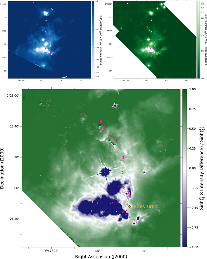
Figure 1. Images centered on the HOPS 361 region. Top left: epoch (1) F160W image with a sinh stretch and (top right) epoch (2) synthetic F160W image with an arcsinh stretch. Bottom: the cropped F160W difference image with a diverging color bar and sinh stretch. Blue (negative values) represents epoch (1), and green (positive values) epoch (2); blue transitioning to green marks a white boundary for a knot potentially moving between epochs. HOPS 361-C is shown with the largest, yellow, star-shaped marker, and other nearby protostellar sources are pink. Knots we identify (Table 2) are numbered for reference, where (1) is closest and (11) is farthest from HOPS 361-C. Our SOFIA 4GREAT beam is shown around knot (1).
Download figure:
Standard image High-resolution imageFor the second epoch images, the closest continuum filter was subtracted from each line image to construct narrowband images in [Fe ii] 1.26 μm and 1.64 μm as well as Paβ 1.28 μm. The appropriate continuum filters were F130N for F126N and F128N, and F167N for F164N. The continuum-subtracted narrowband images from the second epoch are shown in Figure 2.
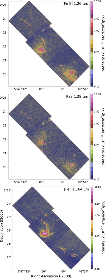
Figure 2. From top to bottom, we show the continuum-subtracted 1.26 μm [Fe ii], 1.28 μm Paβ, and 1.64 μm [Fe ii] mosaics coaligned for ease of comparison. All colorbars use a natural log stretch.
Download figure:
Standard image High-resolution image2.2. SOFIA GREAT
SOFIA observations taken on 2021 February 9–10 use the 4GREAT channel to observe the [O i] 63 μm line. The 4GREAT footprints overlap the HOPS 361 region, and [O i] emission traces the shocked material to give a jet's radial velocity and calibrate shock models, as shown with observations of other emission lines (e.g., Hartmann & Raymond 1984; Carr 1993; Hartigan et al. 2000; Graham et al. 2003) and theoretically for jets exhibiting bow shocks (e.g., Hartigan et al. 1987). The observations have a sensitivity of 0.04 K with 2 km s−1 bins, resulting in a signal-to-noise ratio (S/N) of ∼6.
There is only one pointing that overlaps the base of the HOPS 361-C jet (see the circular region centered on the R.A. and decl. of 05h47m04723, 00d21m5784 in Figure 1). The footprint is shown with a diffraction limited beam size with a radius of 315. After removing the second-order baseline, the resulting [O i] 63 μm line spectrum is shown in Figure 3 with a Gaussian profile that is fit by least squares minimization. The fit gives a mean velocity of 3.3 ± 0.5 km s−1 and a full width at half the maximum value of 15.8 ± 2 km s−1. Comparing the mean velocity with the HOPS 361-C protostar's systemic velocity of 9.5 km s−1, Cheng et al. (2022) yields an average radial velocity at the base of the jet of approximately −6.2 km s−1 and a velocity spread with FWHM of about 16 km s−1.
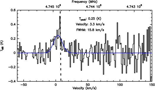
Figure 3. The SOFIA 4GREAT spectrum in black, centered on the [O i] 63 μm line, and positioned near the base of the HOPS 361-C jet. For the footprint on the sky, see Figure 1. The blue curve marks a Gaussian fit to the line centered at around 3.3 km s−1 with parameters listed in the figure. The dashed line shows HOPS 361-C's systemic velocity of 9.5 km s−1 for reference (Cheng et al. 2022).
Download figure:
Standard image High-resolution image3. Identifying Knots and Proper-motion Methods
We used the HST images to identify bright knots of ionized gas in the HOPS 361-C jet and measure their proper motions tangential to the line of sight between the first and second epoch. The images from the two epochs were taken with different filters, so we constructed a synthetic broadband F160W image for the second epoch. We use the second epoch [Fe ii] F164N image, representative of line emission, and the F167N image, corresponding to the continuum, to construct the synthetic F160W image. We set intensities below 0 and above 10−14 to 0 to clip data outside typical knot intensities. We then scale the first epoch image by 9.16 ×10¹⁵, the second epoch image by 8.53 ×10¹⁴, and added 0.168 to the difference. Other linear combinations give similar morphology, but this combination allows the range of intensities for epochs (1) and (2) to be negative and positive respectively.
Our synthetic epoch (2) F160W image is shown in the top right of Figure 1. The Figure 1 bottom panel shows the difference between the first epoch F160W image and the synthetic image from the second epoch. We use this difference image to identify the center of bright knots and measure their proper motions between epochs.
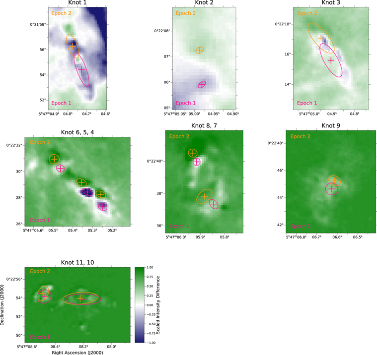
The centers for fast-moving knots are visually identified from regions with strong gradients in the difference image (i.e., white-green or blue-green in Figure 1). Ellipses centered on each knot are adjusted by hand in size and orientation by blinking between the epochs (the upper panels of Figure 1) using SAOImage DS9 software. In Table 2, we show our elliptical regions for each knot, including their coordinates in each epoch as well as their dimensions. For zoomed-in versions of these knots, see Figure 10 in the Appendix.
Table 2. Knot Measurements with Regions
| Knot Identifier | Epoch 1 R.A., Decl. | Epoch 2 R.A., Decl. | Semimajor Axis | Semiminor Axis | AV |
|---|---|---|---|---|---|
| ... | (dd:mm:ss, hh:mm:ss) | (dd:mm:ss, hh:mm:ss) | (arcsec) | (arcsec) | (mag) |
| 1 | 5h47m047278, +0d21m54424 | 5h47m047749, +0d21m56281 | 1.98 | 0.75 | 30.3 ± 1.63 |
| 2 | 5h47m049808, +0d22m05917 | 5h47m049869, +0d22m07256 | 0.32 | 0.22 | 24.0 ± 1.48 |
| 3 | 5h47m049050, +0d22m15608 | 5h47m049488, +0d22m17079 | 2.48 | 0.97 | 9.6 ± 3.85 |
| 4 | 5h47m052484, +0d22m27308 | 5h47m052577, +0d22m28261 | 0.81 | 0.45 | 16.0 ± 0.73 |
| 5 | 5h47m053264, +0d22m28448 | 5h47m053562, +0d22m29181 | 0.83 | 0.49 | 17.1 ± 0.67 |
| 6 | 5h47m054630, +0d22m30251 | 5h47m054940, +0d22m30948 | 0.79 | 0.71 | 20.3 ± 0.97 |
| 7 | 5h47m058456, +0d22m37350 | 5h47m058837, +0d22m37836 | 1.12 | 0.65 | 30.7 ± 1.8 |
| 8 | 5h47m059158, +0d22m39970 | 5h47m059315, +0d22m40507 | 0.62 | 0.56 | 31.4 ± 1.13 |
| 9 | 5h47m066270, +0d22m44653 | 5h47m066131, +0d22m45252 | 0.93 | 0.92 | 20.8 ± 2.04 |
| 10 | 5h47m082013, +0d22m53882 | 5h47m082241, +0d22m53988 | 3.70 | 1.26 | 7.7 ± 8.78 |
| 11 | 5h47m084797, +0d22m54173 | 5h47m084879, +0d22m54500 | 1.69 | 1.06 | 1.9 ± 8.75 |
Note. Knot measurements include central knot coordinates and the ellipse region parameters for each knot. The knot identifiers are number labels for knots, where knot (1) is closest to HOPS 361-C, and knot (11) is the farthest knot. We also show the mean extinction, AV , for each knot with their respective median uncertainties in Figure 8.
Download table as: ASCIITypeset image
We measure proper motions by computing how many pixels each knot's center shifts between epochs. The shifts in units of pixels listed in Table 2 are converted to angular sizes using HST's pixel size (012825) and to physical lengths using the adopted distance of 430.4 pc from Tobin et al. (2020). To find speeds, we divide by the time between epochs (11 yr). Table 3 lists the shifts in arcsecs and the resulting proper motions. Figure 4 illustrates the direction of motion with arrows at the location of each knot.
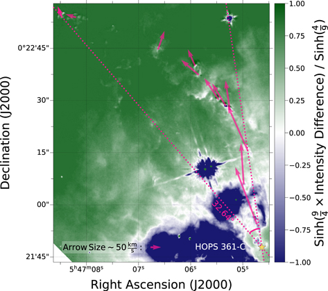
Figure 4. A zoom-in of the difference image from Figure 1 with pink arrows made from our proper-motion measurements (listed in Table 3). The yellow star marker in the bottom right corner is HOPS 361-C, which we assume is the protostellar source for the jet. The labeled angle and dotted lines mark the knots from HOPS 361-C that form an extreme angle.
Download figure:
Standard image High-resolution imageTable 3. Knot Motion and Speeds
| Knot Identifier | R.A. Shift | Decl. Shift | Proper Motion | Tangential Speed (vP ) | Position Angle | Shock Speed (vS ) | Total Outflow Speed (voutflow) |
|---|---|---|---|---|---|---|---|
| ... | (arcsec) | (arcsec) | (arcsec yr−1) | (km s−1) | (°) | (km s−1) | (km s−1) |
| 1 | 0.689 | 1.857 | 0.180 | 290.7 | 20.8 | 51.6 | 342 |
| 2 | 0.078 | 1.339 | 0.122 | 196.6 | 3.9 | 50.2 | 247 |
| 3 | 0.643 | 1.471 | 0.146 | 235.6 | 24.0 | 46.9 | 282 |
| 4 | 0.130 | 0.953 | 0.087 | 141.2 | 8.3 | 50.9 | 192 |
| 5 | 0.440 | 0.733 | 0.078 | 125.5 | 31.4 | 49.1 | 174 |
| 6 | 0.458 | 0.697 | 0.076 | 122.4 | 33.7 | 52.3 | 174 |
| 7 | 0.567 | 0.486 | 0.068 | 109.6 | 49.6 | 52.6 | 162 |
| 8 | 0.230 | 0.537 | 0.053 | 85.8 | 23.7 | 47.8 | 133 |
| 9 | −0.214 | 0.599 | 0.058 | 93.4 | −19.2 | 49.3 | 142 |
| 10 | 0.341 | 0.106 | 0.032 | 52.4 | 72.8 | 49.8 | 102 |
| 11 | 0.120 | 0.327 | 0.032 | 51.1 | 20.6 | 48.5 | 99.6 |
Note. Motion-based values derived for each knot, including how much knot centers move between epochs (see Figure 10), proper motions, and tangential speeds. The knot identifiers are shown as in Table 2, where (1) is the knot closest to HOPS 361-C, and (11) is the farthest. Position angles for the tangential velocity vectors are measured between HOPS 361-C and each knot, relative to celestial north. Shock speeds added with the tangential speeds result in the total flow speed through each knot.
Download table as: ASCIITypeset image
Proper motions for Herbig–Haro (HH) objects can be determined using the centroid for a box surrounding a knot of interest (Bally et al. 2002; Reiter et al. 2017; Erkal et al. 2021), shifting one epoch relative to the next and minimizing the square of the difference summed over a box (Hartigan et al. 2001), by fitting more complex shapes (e.g., a symmetric parabola or Gaussian) to a knot or the jet (Eislöffel & Mundt 1992), or by cross correlation of both images (Reipurth et al. 1992; Raga et al. 2012, 2017). We attempted differently shaped regions, centroids, and phase-based cross correlations but found these methods sensitive to noise, thresholding, and background subtraction. The automated methods are hampered by the different filters between the two epochs and because nonrigid knots broke up or changed shape between epochs. We find that our results are consistent with other methods but produce less noisy knot centers.
Figure 4 shows that the proper motions and arc of knots overall appear consistent with outflows originating from HOPS 361-C. Our result is concordant with prior studies that found proper-motion directions tend to align with a vector to their source (e.g., Anglada et al. 2007). But it is unclear if these knots all originate from the HOPS 361-C jet. To check, we determine extinction to infer each knot's relative location within the cloud, and we confirm whether these knots have shock properties akin to other protostellar jets.
4. Extinction and Shock Modeling
4.1. Observed Extinctions
We need spatially varying extinction measurements in order to interpret line ratios in terms of shock models and to estimate how deeply a protostar and its jet are embedded within the molecular cloud. We estimate extinction with the second epoch [Fe ii] 1.26 μm and [Fe ii] 1.64 μm spectral line images. These lines share a common upper state, so their intrinsic or unextinguished ratio can be computed from the wavelengths and Einstein A-coefficients for the transitions. The primary uncertainty is that the Einstein A-coefficients are difficult to determine theoretically.
We mitigate uncertainties in A-coefficients by adopting an observed zero-reddening value of 2.6 for the [Fe ii] line intensity ratio based on observations of bright HH objects in NGC 1333 (Rubinstein 2021). Next, we use the RV = 5.5 model by Weingartner & Draine (2001) to find an optical depth from the ratio of the observed and theoretical [Fe ii] line intensity ratios. The resulting map of AV for the HOPS 361 region is shown in Figure 5. An S/N of 2 is used to clip any signal in either HST line image below twice the noise of 1.55 × 10⁻¹⁸ erg cm−2 s−1 per pixel from Section 2.1.

Figure 5. AV map of HOPS 361 with an arcsinh stretch. Values are computed using the [Fe ii] 1.26 μm/[Fe ii] 1.64 μm spectral line intensity ratio, with each line image having an S/N >2. HOPS 361-C is shown as a yellow, star-shaped marker.
Download figure:
Standard image High-resolution imageWe use the regions we define in Section 3 to estimate the mean extinction to each knot, both of which are listed in Table 2. For uncertainties, we use the "error" image or uncertainty plane directly outputted by drizzlepac for each image. The uncertainty for each pixel consists of exposure times taking account of Poisson noise (e.g., shot noise), read noise, and other sources of uncertainty. We propagate through the steps of calculating line ratios and extinction. The uncertainties show the extinction is well estimated in the vicinity of HOPS 361-C and the arced jet where we detect proper motions, until the end of the jet where the extinction drops off.
4.2. Shock Speed and Pre-shock Density
The emission-line knots along the HOPS 361-C outflow are HH objects: ionic-line emission follows the passage of a dissociative and ionizing shock produced by supersonic variations in outflow speed or the outflow supersonically interacting with the ambient medium. At each knot, an outflow, initially launched at speed vj and pre-shock hydrogen number density n0, enters a shock at relative speed or shock speed vS . It decelerates and compresses in a (Rankine–Hugoniot) jump to speed vS /4 and density 4n0, then to a lower speed and higher density determined by momentum conservation and radiative cooling.
Post-shock velocity, the vector sum of proper motion vP and radial velocity vR , differs from outflow velocity voutflow by vS . Post-shock ionic-line-emission intensities are sensitive to vS and n0, so vP and vR measurements enable us to determine outflow speed voutflow ≈ vS + vP , mass density ρ0 = μ n0 (μ as the mean molecular weight), mass flux ρ0 v = μ n0 v, momentum flux ρ0 v2, and kinetic energy flux ρ0 v3 lost by the outflow at every knot.
We determine vS
and n0 from observed line emission with the 1D shock and photoionization code MAPPINGS V (Sutherland et al. 2018). For [Fe ii], we substitute the network of [Fe ii] radiative and collisional rate coefficients calculated by Tayal & Zatsarinny (2018), but otherwise use the default atomic–physical data from the CHIANTI database (Del Zanna et al. 2021). The typical protostellar shock speeds are small enough that little sputtering of dust is expected, so we assume the same gas-phase abundances as Watson et al. (2016). We generate a grid of model line-emission spectra with vS
= 20–62 km s−1, and n0 = 0.1–320,000 cm−3. At each grid point, we assume a magnetic field oriented perpendicular to the outflow and frozen into the medium at typical interstellar strength,  . Each calculation terminates at gas temperature T = 100 K. While MAPPINGS is 1D, HH objects are well-resolved structures observed close to edge-on, so the fits to the observed intensity can still estimate vS
and n0.
. Each calculation terminates at gas temperature T = 100 K. While MAPPINGS is 1D, HH objects are well-resolved structures observed close to edge-on, so the fits to the observed intensity can still estimate vS
and n0.
Our model-grid results, derived parameters, and sensitivity to observations are in Figure 6. The intensity ratios are from our HST images. Blue, nearly vertical contour lines can be a ratio of H i Pa β 1.28 μm to either NIR [Fe ii] line. This line ratio is sensitive to vS and relatively insensitive to n0. Green, nearly horizontal contours show the ratio of mid-infrared [Si ii] 34.8 μm and [Fe ii] 26.0 μm emission lines. This ratio is sensitive to n0 and insensitive to vS . The northern half of the jet, imaged with the Spitzer Infrared Spectrograph at 15'' spatial resolution, includes the spectral lines [Fe ii] 26.0 μm and [Si ii] 34.8 μm (Melnick et al. 2008).

Figure 6. Line ratio nomogram from the MAPPINGS V model grid: log([Fe ii] 1.26 μm/H i Paβ 1.28 μm) in blue, log([Fe ii] 26.0 μm/[Si ii] 34.88 μm) in green, plotted against shock speed vS and preshock density n0. The magenta circle indicates the locus of line ratio values with well-defined HH objects in both the HST and Spitzer spectroscopic images. It implies shock speed vS = 45.7 km s−1, and preshock density n0 = 3.2 × 104 cm−3.
Download figure:
Standard image High-resolution imageThree bright regions in the Spitzer images (labeled P1, P2, and P3 in Figure 6 of Melnick et al. 2008) are chosen to measure the [Si ii] 34.8 μm to [Fe ii] 26.0 μm line ratio of ∼0.45. Peaks in the HST images in the same regions are used to measure the ratio of [Fe ii] 1.26 μm to Paβ, about −0.15. These two line ratios are placed on the MAPPINGS shock model in Figure 6 with a pink circle whose size approximates the scatter from differences of ratios at the different peaks. From the location of the pink dot in Figure 6, we estimate n0 ≈ 3.2 × 104 cm−3, and vS = 40–50 km s−1.
HST images may show morphology not evident in relatively lower-resolution Spitzer images. We use the [Fe ii] 1.26 μm to Paβ line ratio, computed from the HST images alone, to create an image that shows the shock speed derived from the MAPPINGS model grid. Taking advantage of the density insensitivity for the NIR [Fe ii]/H i Paβ ratio, we fit a third-order polynomial to our grid points to estimate the shock speed, which is accurate to a few kilometers per second:
where R is the [Fe ii] 1.26 μm/Paβ 1.28 μm intensity ratio. We use this relation to generate the shock-speed image in the bottom panel of Figure 7 with each line image at an S/N above 1. We neglect correcting the [Fe ii] 1.26 μm and Paβ lines for extinction. The two lines are close in wavelength, so the effect of extinction is negligible.
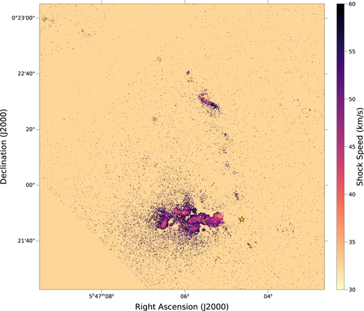
Figure 7. The shock-speed map computed from the [Fe ii] 1.64 μm/H i Pa β 1.28 μm intensity ratio with each line image having an S/N of 1 and using Equation (1). HOPS 361-C is shown as a yellow, star-shaped marker.
Download figure:
Standard image High-resolution imageUnlike proper motions, shock speeds do not appear to depend strongly on distance along the outflow from HOPS 361-C. The shock-speed map in Figure 7 shows the path of knots according to our proper motions may extend farther than about 0.2 pc from HOPS 361-C, following bright trails of molecular hydrogen emission (Walther & Geballe 2019; Eislöffel 2000) and extended line emission in Figure 2. Making conclusions about neighboring frames is difficult without detecting proper motions and bright knots to the southwest of the HOPS 361 clump. There appears to be a strip of shocked material neighboring HOPS 361-E, but the source is unclear in the first epoch. According to our extinction map in Figure 5, this part of the HOPS 361 clump has a higher degree of extinction. Ambiguity remains as the trail may consist of a single arc or form a longer wave as the result of previous periodic ejections in a precessing jet.
5. Discussion
5.1. HOPS 361-C Jet Speed
Using shock speeds (estimated via Equation (1)) and proper motions, we estimate the total outflow speed through each knot. We then examine how outflow speed depends on distance from the HOPS 361-C source. A decrease in flow velocity as a function of distance from the source may be consistent with a jet slowed or decelerated by the host molecular cloud. Such a jet may inject its energy and momentum into its host molecular cloud and locally affect stellar feedback.
To estimate total flow speed, following Coffey et al. (2004), Bally et al. (2002), we sum the 3D velocities of post-shock gas, as measured by the proper motions and radial velocity added in quadrature, with the velocity jump through the shock from Section 4.2. We ignore radial velocity because the majority of the speed is due to the 100–350 km s−1 tangential motions as opposed to the radial velocity of <5 km s−1, so these velocities indicate that the jet is oriented close to the plane of the sky (for examples exploring protostellar jets, their resultant shocks, and inclination effects, see Hartigan et al. 2000; Graham et al. 2003; Jhan et al. 2022). According to the 1D shock model described in Section 4.2, half of the velocity spread of shocked material measured from [O i] in Figure 3 should be between the speed of turbulent gas measured from C18O (1 km s−1; see Iwata et al. 1988; Stanke et al. 2022) and roughly a quarter of the shock speed (10 km s−1). With a velocity spread of 6.2 km s−1, our assumed radial velocity and low inclination are consistent with the model.
In Figure 8, we show quantities for each knot listed in Table 3 as a function of distance from the likely protostellar source, HOPS 361-C. In the top panel, blue triangles show tangential velocity directly found from the proper motions. Yellow x's show the velocity of the shocked gas, estimated from the [Fe ii]/Paβ line ratio. The green dots show the sum of these two quantities, which is an estimate for each knot's total outflow velocity. The red diamond shows the radial velocity for the jet from our SOFIA spectrum in Figure 3.
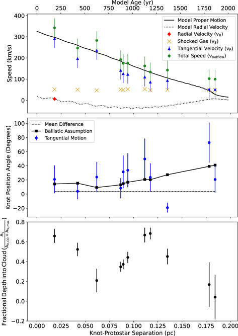
Figure 8. Top: the tangential speed derived from proper motions (blue triangles), shock speed from the [Fe ii]/Paβ line ratio (yellow x's), and bulk speed of the jet and outflow through each knot from adding the two (green dots). A precession model is plotted for the tangential speed (solid curve) and radial velocity (dotted curve). The red diamond shows the observed radial velocity for knot (1) estimated from the [O i] 63 μm spectrum. The modeled time since ejection is shown on top of the plot. Middle: proper-motion position angles relative to celestial north (blue dots), and expected position angles for knots ballistically ejected by HOPS 361-C (black squares). The dashed line is the 4° mean difference between observed and expected angles. Bottom: we estimate each knot's depth within the cloud from the ratio of extinction to the knot and the cloud's total extinction, based on C18O observations. Here, the x-axis shows the direct distance on the sky to the likely protostellar source, HOPS 361-C.
Download figure:
Standard image High-resolution imageThe top panel of Figure 8 shows that the outflow velocity is decelerating as a function of distance from the source. Because proper motions dominate the speed, their uncertainty values are plotted by applying deviations of 2 pixel, from the angular resolution or PSF's FWHM of epoch (1), to the offsets listed in Table 3, which corresponds to a speed of about 44 km s−1. The velocity drops from about 350 to about 100 km s−1 over a distance of 0.2 pc, which may be because of collisions in a dense environment (e.g., Velázquez et al. 2013).
The amount of deceleration is relatively larger than that in more linear jets suspected to also impact into dense gas. For example, HH 1 is noted to have almost no deceleration (<50 km s−1) over a distance of approximately 0.15 pc despite interactions within a dense clump (Raga et al. 2017; Castellanos-Ramírez et al. 2018). HH 2 is similarly noted to not have much or any deceleration over a distance of 0.02 pc after finding low dispersion in over 70 yr of data (Raga et al. 2016).
Jets have knot velocities typically aligned with the direction of their source (e.g., Raga et al. 1993; Heathcote et al. 1996; Schwartz & Greene 1999). In the middle panel of Figure 8, the blue points show the direction of motion for each knot relative to celestial north, based on the proper motions. Black squares show the position angle of the vector between each knot and HOPS 361-C. The uncertainties plotted for the proper motions apply the same worst case scenario using 2 pixel deviations in our measured offsets. The observed velocity vectors have position angles that are about 4° higher than what is predicted if the knots were shot out ballistically (i.e., a straight line on the sky) from HOPS 361-C. That said, our uncertainties cannot rule out ballistic motion on average for the majority of knots except the outlier at approximately 0.13 pc.
In case the discrepancy between the proper motion's direction and direction to source is real, the potential explanations are that the knots are launched by a different protostellar source than HOPS 361-C, a projection effect (e.g., more extreme radial velocities, another protostar launching the knot), or nonballistic motion. We searched for an alternative source but did not find a candidate among the known HOPS 361 protostars (A)–(E) and the nearby protostars HOPS 335 and HOPS 366. The deviation from ballistic motion for the outlier at 0.13 pc could be caused by deflection due to dense clumps of gas in the ambient molecular cloud material, which may change the direction of a knot (Raga & Canto 1995).
5.2. A Decelerating Jet Precession Model
To match the positions and proper motions of our knots of ionized gas, we construct a model similar to those used to model wiggles observed in jets. For background and diagrams of precessing jets, please see Masciadri & Raga (2002), Anglada et al. (2007).
We adapt the analytical model from Raga et al. (2009) and invoke constant jet ejection velocity (Raga et al. 1993) but with an additional damping term (i.e., time-dependent exponential decay) to account for the observed decreasing speeds in Figure 8. The constant density jets with a decaying, time-dependent velocity profile are not without precedent in jet models (e.g., Kofman & Raga 1992; Velázquez et al. 2013), modeling observed radial velocities and proper motions for HH objects (e.g., HH 34 by Cabrit & Raga 2000; HH 80/81/80N by Masqué et al. 2015; HH 223 by López et al. 2015), and modeling knots of CO gas for a moving protostellar source (e.g., PV Cep by Goodman & Arce 2004).
We consider a binary comprised of two stars with masses m1 and m2 in a circular orbit of radius aB . The jet is assumed to be emitted from m1, and the binary orbit lies in the x, y plane. Due to the motion of m1 about the center of mass of the binary system, the initial position from the jet source as a function of ejection time te is

where the binary system's mean angular motion is
Here, the distance from the binary's center of mass position to the jet source, m1, is

The jet precesses if misaligned with the binary orbit's normal (Terquem et al. 1999). The precessing jet then has an initial velocity vector originating from m1
where ϕ0 is a phase with respect to the binary orbit, the angle β sets the opening angle of the jet with respect to the orbital plane, and vj is the jet velocity. The jet is assumed to be ballistic, so the fluid parcels representing knots preserve their velocity at the launch. Here Ωp is the precession rate of the jet. Taking into account the orbital motion of the binary, the initial velocity vector of jet material emitted at te is

We allow the velocity of emitted material to drop as a function of travel time with

where α describes the decay rate. Here v (te ) is given in the previous equation. After a knot is emitted, its direction of motion does not change, so the jet propagates ballistically. However, the velocity of emitted material decelerates due to the α parameter. Without damping (in the limit of α → 0), the model reduces to that by Masciadri & Raga (2002) for orbital motion alone. What is more, if the precession rate is set to zero, or that for precession alone, then binary motion is neglected.
We integrate v (te ) in Equation (6) to find the position of ejected material at a later time t

or specifically
Here the ejection time is te , and the present time of observation is t. By setting the present time t = 0, the angle ϕ0 sets the jet orientation at the present time. We can use Equation (8) to compute the position of ejected material as a function of ejection time and the velocity of this same material using Equation (6). This gives the position and velocity of ejected material in a coordinate system associated with the binary star.
We rotate along the x-axis to correct for the inclination iB of the binary orbit normal vector. Here iB = 0 corresponds to an edge-on binary orbit plane. Then we rotate the resulting coordinate system along the line of sight by angle ξ to correct for the position angle of the binary orbit's normal on the sky.
Coordinates on the sky are xs , zs , and ys , with ys increasing away from the viewer along the line of sight. Here zs is positive to the north, and xs is positive to the west. This is a right-hand coordinate system with origin at the location of the source, HOPS 361-C. The rotations given in Equation (9) are also used to transform the velocity vectors. This gives vxs , vzs for motions in the plane of the sky (tangential motions), and vr = vys corresponding to motion along the line of sight (the radial component). The resulting model has the following free parameters: vj , Ωp , α, β, iB , ξ, ϕ0, m1, m2, aB .
We explore the parameter space by hand to see what ranges of parameters match the knot locations, the decrease in outflow velocity as a function of distance from the source protostar and the radial velocity of the first knot. We do not attempt to fit the semimajor axis (aB ) or masses of the orbit's constituents (m1, m2) because these parameters only change the jet trajectory on scales smaller than observed, but we still allow the binary to change the jet's behavior. Lower inclinations relative to the plane of the sky (0°–5°; see Section 5.1) narrowed our search through the parameter space and better matched positions on the sky, proper motions, and opening angle (Figure 4). The first knot's low radial velocity (Section 2.2) and our measured proper motions were better matched with low initial phase angles (10 < ϕ0 < 20).
We could not find a model that results in the observed deceleration (see Section 5.1) via projection effects alone. Models with an extreme opening angle, wider than what we measure in Figure 4 (33°), can exhibit a drop in proper motion as a function of distance from the source protostar. However, if our observed deceleration was caused by knots moving away from the observer, then the model knot positions predicted on the sky tend to be closer to the source than observed. We find that precessing jet models only match knot locations and velocities when the ejected knots rapidly decelerate, as described with our exponential decay parameter α. The models that match the positions and proper motions have half opening angle of β ≈ 15° and require moderate α values within about 20% of that given in the Table 4. Such a model is shown in Figures 8 and 9 and has parameters listed in Table 4.
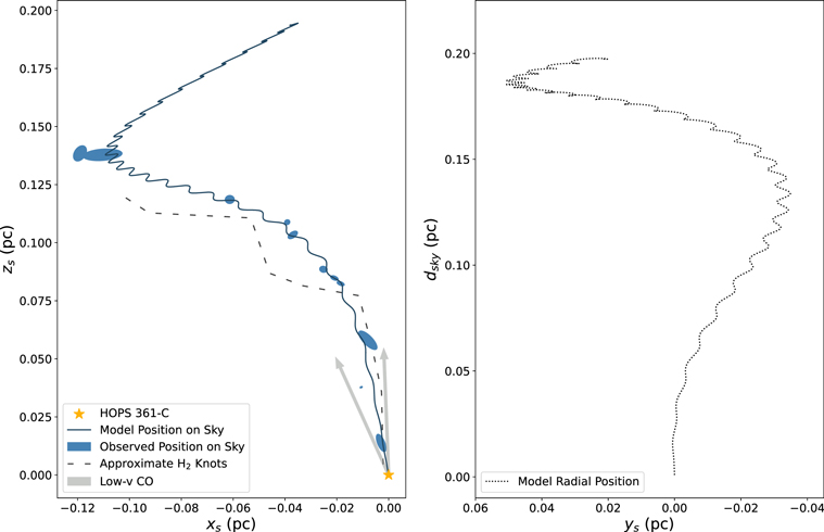
Figure 9. Left: knot regions on the sky in xs , zs (pc) are plotted as blue ellipses with a jet precession model shown by a solid black curve. Model parameters are listed in Table 4. Here, celestial north points up, and east to the left. The yellow star on the bottom right marks the jet source as in Figure 4 and is placed at the origin. Molecular hydrogen knots from Walther & Geballe (2019) are approximated by a dashed curve, and the low-velocity CO cavity from Cheng et al. (2022) is shown with gray arrows. The molecular hydrogen may mark a helix of gas accelerated by the jet, but we lack data to confirm this. The low-velocity CO gases encompasses a high-velocity CO jet and a radio continuum jet (Trinidad et al. 2009; Carrasco-González et al. 2012) that respectively align with the molecular outflows and the beginning of our track of [Fe ii] knots. Right: the ys -coordinates for knots predicted from our model are shown with a dotted curve as a function of distance on the sky from the source, dsky. The ys -coordinate gives distance along the line of sight with origin at the source and with positive ys more distant from the viewer.
Download figure:
Standard image High-resolution imageTable 4. Precessing Jet Model Parameters
| Parameter | Symbol | Fiducial Values |
|---|---|---|
| Jet ejection velocity | vj | −325 km s−1 |
| Precession period | 2π/∣Ωp ∣ | 2066 yr |
| Jet decay rate | α | 1560 Myr−1 |
| Half jet opening angle | β | 14 5 5 |
| Binary orbit inclination | iB | 0° |
| Position angle of precession axis | ξ | 235 + 180° |
| Initial phase | ϕ0 | 1275 |
| Mass of jet source | m1 | 1 M⊙ |
| Mass of binary companion | m2 | 1 M⊙ |
| Binary semimajor axis | aB | 20 au |
Download table as: ASCIITypeset image
Figure 9 shows knot positions on the sky from Table 2 as blue ellipses in the left panel. The black curve represents our model jet trajectory from HOPS 361-C. The plot axes xs and zs give coordinates on the sky in parsecs with origin at the jet source, which is shown with a fuchsia star. Celestial north is aligned with zs , so it is facing up on this panel. A knot location can be used to estimate the time a knot was ejected from the source. The ejection times, estimated from this model, are shown on the top axis of Figure 8.
The molecular hydrogen knots from Walther & Geballe (2019) are shown by an approximate dashed curve, and the low-velocity CO cavity from Cheng et al. (2022) is shown with gray arrows. The helix of molecular hydrogen may be accelerated by the jet that we detect but cannot presently be analyzed in detail because of imaging differences (e.g., other protostars could heat gas, differences in brightness and epochs). We caution that past observations strictly correspond to any of the densest and warmest parts of the gas. The low-velocity CO gas encapsulates high-velocity CO gas and a jet of radio continuum emission from Trinidad et al. (2009), Carrasco-González et al. (2012) aligning with the molecular hydrogen knots and lying on top of the track of our detected [Fe ii] knots.
The right panel in Figure 9 shows the ys coordinate of the model jet trajectory as a function of distance on the sky from the source (dsky) as in Figure 8. Along the line of sight, the increasing ys corresponds to greater depths into the cloud. With our model, the jet is moving toward then away from the observer as a function of dsky.
HOPS 361-C was only recently resolved as a close binary system in VLA 9 mm continuum images with a model binary separation of about 01 or 43 au (Cheng et al. 2022). Following Terquem et al. (1999), the binary system's orbital period is related to the jet's precessional period, assuming a rigid disk of gas within the binary system that precesses, uniform disk surface density, and Keplerian orbits,

where τorbit is the binary orbital period, q = m2/m1 is the ratio of the secondary mass divided by the primary, which is assumed to be the jet source. Here σ is the ratio of m1's disk radius to the binary orbital semimajor axis. Typically, σ is taken to be 1/3, assuming tidal truncation; though it could range from 1/4 to 1/2.
We found precession models match positions and proper-motion data with periods of 2π/∣Ωp ∣ ranging from about 1500 to 2500 yr. With a 2000 yr precession period, a binary star comprised of two 1 M⊙ stars (q = 1) has an orbital period of 130 yr and a semimajor axis of 33 au, which is approximately consistent with the separation inferred from the VLA 9 mm images. However, kinematic modeling of molecular line emission gave an inner disk radius that is smaller, 10–25 au (Cheng et al. 2022). If this inner radius encompasses the binary, then the binary semimajor axis would necessarily have to be smaller than the inner disk radius.
We note the precession model shown in Figures 8 and 9 is not sensitive to the binary separation or the mass of its constituents; though the small amplitude wiggles in the model curves are due to the binary orbital motion. With a larger binary separation, these wiggles would have lower amplitude and longer wavelength.
Via kinematic modeling, Cheng et al. (2022) estimate a binary mass for HOPS 361-C of m1 + m2 ∼ 1.5M⊙; though modeling the spectral energy distribution gave a protostellar mass of ∼2M⊙ neglecting binarity. These estimates for the protostellar masses are similar to our assumed values of m1 = m2, and m1 + m2 = 2M⊙. Based on an estimate for the location of the kinematic center, Cheng et al. (2022) estimate a mass ratio m1/m2 ≈ 1.3 −2.5, which is within a factor of 2 of our assumed value of m1/m2 = 1. Using our current measurements and uncertainties, the jet precession model is not inconsistent with what is known about the HOPS 361-C binary system.
The direction of precession is predicted to be in the opposite direction as the rotation of the disk from which the jet originates (Ωp is negative in Equation (1) by Terquem et al. 1999). Since the precession rate is computed by averaging the tidal force over the binary's orbit, it is independent of the direction of rotation in the binary orbit. We take Ωp < 0 so that position angle and inclination are given with respect to the binary orbit normal. We assume the direction of rotation for the disk driving the jet is similar to the direction of rotation of the binary orbit (for which we chose β < π/2). The position angle of the precession axis, ξ, is also the position angle of the binary orbit normal. This axis points to the south, consistent with the direction of rotation seen in the disk resolved by Cheng et al. (2022).
The CO J = 2−1 data for HOPS 361-C also show a high-velocity, bipolar jet with a position angle of 22°–32°. This differs from the radio jet axis seen at 9 mm that has a position angle of ∼15° (Cheng et al. 2022). Near the source, our precession model has the jet oriented near its maximum opening angle, giving a jet position angle of about 10° and approximately consistent with the radio jet axis.
The jet opening angle β is sensitive to the solid angle extended by the arc with respect to our origin, the protostellar source. The model is less sensitive to the binary inclination iB , but we found models that matched both proper motions and knot positions with iB < 25°. The radial velocity from the [O i] spectrum restricted iB to a few degrees. Cheng et al. (2022) fit kinematic models to their ALMA molecular line data for the HOPS 361-C disk–jet system, and they estimated a disk inclination of 63°–77° and a position angle of around 15° for the radio jet. If we assume their disk inclination is that of a circumbinary disk in a plane containing the binary, this inclination corresponds to iB ∼ 90° − 70° = 20° for the inclination of the binary orbit normal vector using our variable, which has zero inclination for an edge-on binary orbit. Our precession model is consistent with the estimates for the disk inclination by Cheng et al. (2022), assuming their model pertains to a circumbinary disk.
The disk resolved by Cheng et al. (2022) has a blueshifted component on the western side and redshifted component on the eastern side, which suggests that the binary orbit's angular momentum vector is pointed to the south. To compare, if the binary orbit and the disk that drives the jet have the same direction of rotation (opening angle β < π/2), then the jet's arc is part of a counter-jet that propagates in the direction opposite to the binary orbit's normal. The position of the counter-jet can be predicted using Equation (4) with vj < 0, giving the expected S-shaped symmetry about the origin between jet and counter-jet. This is why we have chosen negative vj for our model in Table 4.
The direction of precession in our model is consistent with a disk-driven jet having rotation direction similar to the presumed circumbinary disk observed in various molecular lines by Cheng et al. (2022). We concur with Cheng et al. (2022), who concluded that jet precession and associated interactions between jet and environmental material at different times are the most likely scenario accounting for the observed differences in the jet position angles seen with different tracers.
5.3. Outflow Depth in Surrounding Environment.
We achieve a quasi-3D positioning of the knots by comparing foreground extinction to each knot in Figure 8 (or see Table 2) with the extinction to material at the back of the molecular cloud. Their ratio gives an approximate value for how deeply embedded each knot is within the cloud. But the relative distances may change due to radial distance, column density, number density, or opacity. Therefore, they may not directly correspond to the radial positions predicted by our precession model (the right panel of Figure 9).
The extinction to the back of the cloud can be determined using molecular gas, like optically thin CO isotopologues, that traces relatively slow motions (e.g., Dickman 1975, 1978; Goldsmith et al. 1992; Schwartz et al. 1983; Gutermuth et al. 2008; Stojimirović et al. 2008). We use the correlation between extinction and C18O (J = 1–0) molecular line emission (Alves et al. 1999):

The region of the integrated C18 O map from Iwata et al. (1988) that overlaps our NIR images gives a brightness temperature of 2.52–2.8 K km s−1, which corresponds to an AV of 13.9–15.2 mag using Equation (11). We only find a single value for the region because the radio observations have a nearly 1' spatial resolution, nearly the scale of our jet. We could use C18 O data in Schwartz et al. (1983), but their column density maps have fewer contour lines to use for measurements.
We present the fraction of each knot's AV relative to total AV through the cloud in the bottom panel of Figure 8. Translating the contours from Iwata et al. (1988) to an AV value with the correlation from Alves et al. (1999) introduces an additional uncertainty of approximately ±1.6 mag to the uncertainties in the extinction, and we have used this uncertainty to estimate the error bars for the points plotted in the bottom panel of Figure 8.
The fractional depths in the bottom panel of Figure 8 indicate knots oscillate between being more and less embedded, potentially moving closer and farther from the viewer. We take caution making firm constraints with our precession model, since the cloud is unlikely to be perfectly uniform (e.g., Schwartz et al. 1983). But precession may impact jet morphology and dynamics more than variations in a jet's gas density (e.g., Castellanos-Ramírez et al. 2018). Quantitatively, the knots are at a fractional depth of 1/5–4/5 into the molecular cloud, where they may disrupt the HOPS 361 region.
5.4. Jet Mass, Momentum, and Energy Injection
We search for effects that connect jet properties relevant to stellar feedback, our precession model values, and HOPS 361 cloud clump properties. Assuming a 1D, incompressible fluid flow and mass conservation across each knot (ignoring changes in viscosity, plasma density, and mass flow rate) as in the MAPPINGS model, the jet has a mass outflow rate or jet output ( ) of
) of

and the momentum flux ( ) or ram pressure through each knot for constant
  as
as

and a flux of kinetic energy ( ) or energy density dissipated in the shock in each knot with constant
  of
of

Here ρjet is the jet's mass density, voutflow is total flow speed through each knot, vP
is knot proper motion, vS
is shock speed, and A is the jet's cross-sectional area. We compute  , taking Rknot to be the semiminor axis from Table 2 for an ellipse encircling each knot. As in Section 4.2, we estimate voutflow from the sum of the knot proper motion and shock speed. Assuming the majority of the jet's mass consists of neutral atomic hydrogen, we find the mass density by multiplying the jet's number density (n0 ≈ 3.2 × 104 cm−3, or see Section 4.2) by the mass of a hydrogen atom and using a mean molecular weight of 1. We estimate the total mass density in the jet is ρjet = 5.34 × 10⁻²⁰ g cm−3 = 789 M⊙ pc−3. We list each knot's
  ,
,  , and
, and  multiplied by area A for ease of comparison in Table 5.
Table 5. Derived Feedback Properties for Each Knot
| Knot Identifier | A |

| Δ × A × A
|

|
|---|---|---|---|---|
| ... | pc2 | M⊙ yr−1 | M⊙ yr−1 km s−1 | L⊙ |
| 1 | 7.69 × 10⁻⁶ | 2.12 × 10⁻⁶ | 1.10 × 10⁻⁴ | 5.69 |
| 2 | 6.62 × 10⁻⁷ | 1.32 × 10⁻⁷ | 6.61 × 10⁻⁶ | 0.240 |
| 3 | 1.29 × 10⁻⁵ | 2.93 × 10⁻⁶ | 1.38 × 10⁻⁴ | 5.85 |
| 4 | 2.77 × 10⁻⁶ | 4.29 × 10⁻⁷ | 2.19 × 10⁻⁵ | 0.598 |
| 5 | 3.28 × 10⁻⁶ | 4.62 × 10⁻⁷ | 2.27 × 10⁻⁵ | 0.558 |
| 6 | 6.90 × 10⁻⁶ | 9.72 × 10⁻⁷ | 5.08 × 10⁻⁵ | 1.24 |
| 7 | 5.78 × 10⁻⁶ | 7.56 × 10⁻⁷ | 3.97 × 10⁻⁵ | 0.885 |
| 8 | 4.29 × 10⁻⁶ | 4.62 × 10⁻⁷ | 2.21 × 10⁻⁵ | 0.397 |
| 9 | 1.16 × 10⁻⁵ | 1.33 × 10⁻⁶ | 6.57 × 10⁻⁵ | 1.27 |
| 10 | 2.17 × 10⁻⁵ | 1.79 × 10⁻⁶ | 8.91 × 10⁻⁵ | 1.13 |
| 11 | 1.54 × 10⁻⁵ | 1.24 × 10⁻⁶ | 5.99 × 10⁻⁵ | 0.740 |
Note. Jet properties used to evaluate how the HOPS 361-C jet affects its host cloud. The cross-sectional area derives from squaring the smaller, minor axis of the ellipse centered on each knot and using values from Table 2. The flow speeds needed for other columns are listed in Table 3.
Download table as: ASCIITypeset image
According to Watson et al. (2016), Sperling et al. (2021), the jet output efficiency is the ratio of the mean mass outflow rate through the jet to the accretion rate. Mass accretion rate can be estimated for class 0 and class I protostars using bolometric luminosity (Lbol) and stellar properties (mass, M*, and luminosity, L*) by assuming that the bolometric luminosity is equal to the total luminosity for the binary system as well as the accretion luminosity; then

(Enoch et al. 2009; Evans et al. 2009), where η is an efficiency factor often assumed to be on the order of 1 (Meyer et al. 1997; Calvet & Gullbring 1998; Muzerolle et al. 2003; Fischer et al. 2017). Using the methods from Furlan et al. (2016) to estimate bolometric luminosity, Cheng et al. (2022) estimated a mass accretion rate of 9 × 10⁻⁶
M⊙ yr−1 for HOPS 361-C. Using, the mean  from Table 5 of 1.15 ×10⁻⁶
M⊙ yr−1 and the above accretion rate estimate, we find an efficiency of 0.128. Efficiency is related to the location of the jet launching site, with larger efficiencies corresponding to launch at a smaller radius (Watson et al. 2016; Sperling et al. 2021). Based on Watson et al. (2016), Sperling et al. (2021), the values around 0.1 cannot rule out any jet launching models. If the bolometric luminosity is split between the components of the binary system, then the efficiency may increase, and the jet launching models that place the footpoint closer to the protostar may better explain why our value exceeds 0.1.
from Table 5 of 1.15 ×10⁻⁶
M⊙ yr−1 and the above accretion rate estimate, we find an efficiency of 0.128. Efficiency is related to the location of the jet launching site, with larger efficiencies corresponding to launch at a smaller radius (Watson et al. 2016; Sperling et al. 2021). Based on Watson et al. (2016), Sperling et al. (2021), the values around 0.1 cannot rule out any jet launching models. If the bolometric luminosity is split between the components of the binary system, then the efficiency may increase, and the jet launching models that place the footpoint closer to the protostar may better explain why our value exceeds 0.1.
We determine the momentum injection rate through the jet imparted into the surrounding cloud, compare with escape velocity, and find the amount of mass the jet ejects from the HOPS 361 clump (as in Matzner 2007; Arce et al. 2010; Li et al. 2020). We sum  values for each knot listed in Table 5. Because the interaction with the surroundings may not be perfectly efficient or uniform, then the total force is ≤6.26 ×10⁻⁴
M⊙ yr−1 km s−1. Taking the clump as a uniform, nonrotating, nonmagnetic, spherical mass of Mc
= 88.9 M⊙, at a radius of Rc
= 0.2 pc (using the Herschel map of Orion B described in Stutz & Gould 2016; Stutz p. com.; and Furlan et al. 2016; and the correlation between N(H) and extinction found by Pillitteri et al. 2013), and then the clump's escape velocity (vesc) is 2 km s−1. The ratio of the sum of momenta from the jet's knots to this escape velocity gives
values for each knot listed in Table 5. Because the interaction with the surroundings may not be perfectly efficient or uniform, then the total force is ≤6.26 ×10⁻⁴
M⊙ yr−1 km s−1. Taking the clump as a uniform, nonrotating, nonmagnetic, spherical mass of Mc
= 88.9 M⊙, at a radius of Rc
= 0.2 pc (using the Herschel map of Orion B described in Stutz & Gould 2016; Stutz p. com.; and Furlan et al. 2016; and the correlation between N(H) and extinction found by Pillitteri et al. 2013), and then the clump's escape velocity (vesc) is 2 km s−1. The ratio of the sum of momenta from the jet's knots to this escape velocity gives  esc for material escaping the cloud equal to 3 ×10⁻⁴
M⊙ yr−1, assuming constant escape velocity and momentum output. Over a typical protostellar lifetime or a freefall timescale of 100,000 yr, then the jet would launch approximately 30 M⊙ out of the system, or about a third of the clump's mass. Therefore, a few precessing jets from intermediate-mass protostars may have enough momenta to eject the majority of the clump's mass at this scale.
esc for material escaping the cloud equal to 3 ×10⁻⁴
M⊙ yr−1, assuming constant escape velocity and momentum output. Over a typical protostellar lifetime or a freefall timescale of 100,000 yr, then the jet would launch approximately 30 M⊙ out of the system, or about a third of the clump's mass. Therefore, a few precessing jets from intermediate-mass protostars may have enough momenta to eject the majority of the clump's mass at this scale.
To find the effect of the jet's kinetic energy, we sum power ( ) emitted by each knot in Table 5 to get a total of 18.6 L⊙. The gravitational potential energy of an extended mass or cloud, Mc
, with radius, Rc
, is generally
) emitted by each knot in Table 5 to get a total of 18.6 L⊙. The gravitational potential energy of an extended mass or cloud, Mc
, with radius, Rc
, is generally

where C is a constant dependent on the cloud's geometry and uniformity. Assuming the mass and radius to compute our escape velocity, Equation (16) gives 1.21 × 1045 erg. If the cloud is virialized and only has a total of half of this energy, then the ratio of half of U to  is a 480 yr timescale. This timescale may suggest a precessing jet contributes a significant portion of a cloud clump's gravitational energy budget during a protostellar lifetime. We caution this is the fastest possible case with our present assumptions (perfectly efficient energy transfer, uniform cloud, constant output).
The jet's power may contribute to turbulence within the molecular cloud. The dissipation rate due to turbulence at a velocity of vturb in the molecular cloud is

where leddy is the size of the largest eddies within the cloud (e.g., Stone et al. 1998; Elmegreen & Scalo 2004; Quillen et al. 2005). Taking the NGC 2071 cloud mass Mc ∼ 2000 M⊙and leddy ∼ 1 pc (from 12CO and 13CO maps; see Stojimirović et al. 2008), vturb ∼ 1.9 km s−1 (based on C18O line widths by Iwata et al. 1988; and Stanke et al. 2022; also a velocity FWHM of 1 km s−1 from an NH3 line map using the Green Bank Telescope, by priv. comm. with J. Di Francesco), and then we estimate a turbulent dissipation luminosity of about 2.3 L⊙. Because the knots deliver an average power of about 1.69 L⊙ into the cloud, the energy dissipation rate via turbulence in the cloud is similar to the average power dissipated locally by the jet. The jet itself may have enough energy to locally drive the molecular cloud turbulence.
The HOPS 361-C jet may have enough momentum and energy to disrupt the HOPS 361 protostar-forming clump, but that depends on how efficiently the jet outputs material over time. The jet dissipates over a distance of ∼0.2 pc (Figures 8 and 9). A knot launched at 325 km s−1 traveling 0.2 pc is a dynamical timescale of 600 yr, which is similar to our damping timescale, the reciprocal of α, of 640 yr. The damping or dynamical timescale for knots can occur about 3 times within our precession timescale of 2000 yr, so the jet may extend farther as seen in Figure 2. However, the knots outside this 0.2 pc distance may be due to other outflows or may be associated with lower-velocity shocks <20 km s−1, so future observations are needed to determine their source. Our study of the arced jet associated with HOPS 361-C suggests the precessing jets with wide opening angles are locally damped within 0.2 pc of their driving source.
5.5. Criterion Allowing a Protostellar Jet to Puncture a Molecular Cloud
What condition allows subsequently emitted clumps in a jet to dissipate or remain within the cavity opened by previously emitted clumps? For small opening angles, the clumps in protostellar outflows lie on a similar path as the jet itself, and these jets open a cavity within a molecular cloud (Quillen et al. 2005; Cunningham et al. 2009a; Frank et al. 2014; Fendt & Yardimci 2022). Long jets with small wiggles can puncture their host molecular cloud (e.g., simulations by Velázquez et al. 2013) and extend more than 1 pc from their source (Bally 1982, 2016). In contrast, instead of passing through the molecular cloud, the HOPS 361-C jet seems to entirely dissipate locally within it.
We estimate the speed that a cavity is opened by a jet and compare it to its advance speed. The radial distance and radial velocity from the jet's central axis of symmetry are


where vj is the jet speed, and β is the half opening angle. A jet cavity that would not fill in at the speed of sound, cs , in the ambient molecular cloud would satisfy

This corresponds to a jet cone that moves perpendicular to its central axis slower than the sound speed. Combining this equation with Equation (19), a jet cavity that does not fill in would satisfy

Using a jet velocity of vj =400 km s−1 and a sound speed for the cloud's interstellar medium in the of cs ∼ 1 km s−1, we estimate the half opening angle β ≲ 1° for a jet that can maintain a cavity. In this scenario, any jet traveling at a few 100 km s−1 within an opening angle of a degree requires motions above the local sound speed to fill in the associated cavity. If the opening angle is larger than a degree, then the cavity would fill in. Opening a cavity requires energy. A jet with a wide opening angle may then expend more energy to propagate. This suggests wider jets would dissipate more rapidly, and long jets with large opening angles should be rare.
This scenario ignores turbulence and magnetic fields. But note that the supersonic, turbulent speed of gas in the interstellar medium is approximately Mach 3, where the Mach number is the ratio of motion in the cloud to the local sound speed (Ballesteros-Paredes et al. 2007). To take into account turbulence in the molecular cloud, we multiply the right-hand side of Equation (21) by a factor of 3, and this would relax the restriction on the opening angle for a jet that can puncture a molecular cloud.
2D magnetohydrodynamic simulations have investigated how a precessing jet nozzle affects the propagation of a high-speed jet (Fendt & Yardimci 2022). The jets with wide opening angles (>20°) fail to propagate to large distances as they are dissipated locally (see their Figure 6) but suggest the condition allowing a jet to propagate is less restrictive than that by Equation (21). Future simulations could relate protostellar jet observations (e.g., knot proper motions) to other cloud, jet, and binary properties and elucidate connections between the jet opening angle and jet dissipation. Simultaneously observing molecular, atomic, and ionized components of the HOPS 361-C jet, including potential follow-up for proper motions, may also confirm H2 knots accelerated and carved out by HOPS 361-C.
6. Conclusion
We study new narrowband HST images of the NGC 2071 IR/HOPS 361 star-forming region. To summarize the results, the proper motions of 350–100 km s−1 suggest the arc of knots bright in [Fe ii], which rapidly decelerate away from NGC 2071 IR, appear to trace back to the protostar HOPS 361-C. We measured a radial velocity of 3 km s−1 using a new SOFIA [O i] 63 μm spectrum near the jet's base and found this jet is nearly in the plane of the sky. The knots with proper motions are also confirmed to be shocked with typical speeds of 50 km s−1 and densities of 3 × 104 cm−3, and from extinctions they are embedded at depths of 1/5–4/5 into the cloud.
We apply the precession model by Masciadri & Raga (2002) to infer the full kinematics of the jet from the knot positions, knot speeds, and measured opening angle of 16°. We need an additional parameter to describe the jet's deceleration, assuming the jet has a constant ejection velocity. Our model supports prior proposals that this jet is precessing with a period of 2000 yr, and this is consistent with binary system properties estimated for HOPS 361-C (Cheng et al. 2022). A knot at 0.13 pc from HOPS 361-C may have been deflected, launched by another protostar, or be a spurious motion.
Instead of precession due to the secondary in a binary system, an arc of knots can alternatively be produced by asymmetric infall of the envelope onto the protostar (Hirano & Machida 2019; Lee 2020) or tidal encounters (Cunningham et al. 2009a). Observing the binary source and its envelope could help differentiate asymmetric infall, and future radial velocity measurements for more distant knots confirming or rejecting our model could test whether another option to induce precession is more viable. Another epoch of observations for the wider field for knots more distant than 0.2 pc from the source (on the sky) would enable measuring proper motions, which would show whether the proper motions have dissipated rapidly, or perhaps if more distant knots are associated with outflows from a different protostar.
The HOPS 361-C jet illustrates how jet precession can affect stellar feedback and the host cloud. The lower shock velocities past the end of the arc and more than 0.2 pc from HOPS 361-C suggest that the jet may have almost entirely dissipated at this distance. This is consistent with local and rapid decay of the jet's kinetic energy except if the jet's ejection velocity increases with time. Prior studies have investigated protostellar outflow-induced feedback into molecular clouds (e.g., Matzner 2007; Carroll et al. 2009; Raga et al. 2009; Federrath et al. 2014; Frank et al. 2014; Nakamura & Li 2014; Rohde et al. 2022). The short 0.2 pc dissipation length in HOPS 361-C's jet and total kinetic energy suggest that precessing binary systems could sustain and affect the distribution of length scales for outflow-induced turbulent energy injected into NGC 2071 IR.
Since many known jets with constant direction or small opening angles extend much farther than 0.2 pc, and do not decrease as quickly in velocity as a function of distance from their source (e.g., Lee 2020; Erkal et al. 2021), we suspect that the rapid deceleration we see in the HOPS 361-C jet arc is associated with the jet's wide opening angle. If so, the momentum and kinetic energy in a wide opening angle precessing jet can be imparted to the molecular cloud closer to the jet source than that of a narrow opening angle jet. Future models, building on simulations of precessing jets (e.g., Fendt & Yardimci 2022), could explore how the binary stars that produce precessing jets at different outflow rates impact feedback into molecular clouds.
We thank Eric Blackman and Jonathan Carroll-Nellenback for discussions. We are grateful to Liam Hainsworth for calculating MAPPINGS model grids. Finally, we thank our referee's insights and perspectives.
This research is based on observations made with the NASA/ESA Hubble Space Telescope obtained from the Space Telescope Science Institute (STSci), which is operated by the Association of Universities for Research in Astronomy, Inc., under NASA contract NAS 5-26555. These observations are associated with programs 11548 and 16493. A.E.R., N.K., and S.F. were supported by funding from STScI from program 16493.
The data in this paper are obtained from the Mikulski Archive for Space Telescopes (MAST) at the STSci. The specific observations analyzed can be accessed via 10.17909/e0g3-wc67 and 10.17909/fwz1-0q60.
This work is based in part on observations with the NASA/DLR SOFIA. SOFIA is jointly operated by the Universities Space Research Association, Inc. (USRA), under NASA contract NNA17BF53C, and the Deutsches SOFIA Institut (DSI) under DLR contract 50 OK 2002 to the University of Stuttgart.
This work uses Montage, which is funded by the National Science Foundation (grant No. ACI-1440620). Montage was previously funded by the NASA Earth Science Technology Office, Computation Technologies Project, under cooperative agreement No. NCC5-626 between NASA and Caltech.
Appendix: Knot Close-ups Over Time
In Figure 10, we zoom onto knots identified from the difference image (Figure 1) to better show how each one moves between epochs.
Figure 10. Close-ups of knots identified from the difference image in Figure 1. Epoch (1) is shown in pink, and epoch (2) is shown in orange. Ellipses show the regions associated with each epoch and knot. Pairs of + marks are the positions from Table 1, which generally move up or to the left. The direction of motion and pixel shifts in Table 3 are measured with a line connecting the + marks for each knot.
Download figure:
Standard image High-resolution image