


Abstract
We present images and a multiwavelength photometric catalog based on all of the JWST NIRCam observations obtained to date in the region of the Abell 2744 galaxy cluster. These data come from three different programs, namely, the GLASS-JWST Early Release Science Program, UNCOVER, and the Director's Discretionary Time program 2756. The observed area in the NIRCam wide-band filters—covering the central and extended regions of the cluster, as well as new parallel fields—is 46.5 arcmin2 in total. All images in eight bands (F090W, F115W, F150W, F200W, F277W, F356W, F410M, and F444W) have been reduced adopting the latest calibration and reference files available. Data reduction has been performed using an augmented version of the official JWST pipeline, with improvements aimed at removing or mitigating defects in the raw images and improving the background subtraction and photometric accuracy. We obtain an F444W-detected multiband catalog, including all NIRCam and available Hubble Space Telescope data, adopting forced-aperture photometry on point-spread-function-matched images. The catalog is intended to enable early scientific investigations and is optimized for the study of faint galaxies; it contains 24,389 sources, with a 5σ limiting magnitude in the F444W band ranging from 28.5 AB to 30.5 AB, as a result of the varying exposure times of the surveys that observed the field. We publicly release the reduced NIRCam images, associated multiwavelength catalog, and the code adopted for 1/f noise removal with the aim of aiding users in familiarizing themselves with JWST NIRCam data and identifying suitable targets for follow-up observations.
Export citation and abstract BibTeX RIS

Original content from this work may be used under the terms of the Creative Commons Attribution 4.0 licence. Any further distribution of this work must maintain attribution to the author(s) and the title of the work, journal citation and DOI.
1. Introduction
In just a few months of observations, JWST has demonstrated its revolutionary scientific capabilities. Early observations have shown that its performance is as or better than expected, with an image quality and overall efficiency that matches or surpasses prelaunch estimates (Rigby et al. 2023). Publicly available data sets obtained by the Early Release Observations and Early Release Science programs have already enabled a large number of publications based on JWST data, ranging from exoplanets to the distant universe.
In particular, many works exploited the power of NIRCam to gather the first sizeable sample of candidates at z ≥ 10 (e.g., Bouwens et al. 2023; Castellano et al. 2022; Finkelstein et al. 2022; Morishita & Stiavelli 2023; Naidu et al. 2022; Roberts-Borsani et al. 2023; Robertson et al. 2023; Yan et al. 2023; Castellano et al. 2023; Donnan et al. 2023), demonstrating the power of JWST in exploring the universe during the reionization epoch.
In this paper, we present the full data set obtained with NIRCam in the region of the z = 0.308 cluster Abell 2744, which will significantly expand the available area for deep extragalactic observations. The central region of the cluster allows an insight into the distant universe at a depth and resolution superior to those of NIRCam in blank fields, with the lensing magnification assistance. The data analyzed here are obtained through three public programs: (i) GLASS-JWST-ERS-1324 (Treu et al. 2022), (ii) UNCOVER JWST-GO-2561 (Bezanson et al. 2022), and (iii) the Director's Discretionary Time Program 2756, aimed at following up a supernova discovered in GLASS-JWST NIRISS imaging. We have analyzed and combined the imaging data of all these programs and obtained a multiwavelength catalog of the objects detected in the F444W band.
In order to facilitate the exploitation of these data, we release reduced images and an associated catalog on our website and through the Mikulski Archives for Space Telescopes (MAST). This release fulfills and exceeds the requirements of the Stage I data release planned as part of the GLASS-JWST program. It is anticipated that a final (Stage II) release will follow in approximately one year, combining additional images scheduled in 2023, and taking advantage of future improvements in data processing and calibrations.
This paper is organized as follows. In Section 2, we present the data set and discuss the image-processing pipeline. In Section 3, the methods applied for the detection of the sources and the photometric techniques used to compute the fluxes are presented. Finally, in Section 4, we summarize the results. Throughout the paper, we adopt AB magnitudes (Oke & Gunn 1983).
2. Data Reduction
2.1. Data Set
The NIRCam data analyzed in this paper are taken from three programs that targeted the z = 0.308 cluster Abell 2744 (A2744 hereafter) and its surroundings. The first set of NIRCam images was taken as part of the GLASS-JWST survey (Treu et al. 2022), in parallel to primary NIRISS observations on 2022 June 28–29 and to NIRSpec observations on 2022 November 10–11. We refer to these data sets as GLASS1 and GLASS2, or collectively as GLASS, both of which consist of imaging in seven broadband filters from F090W to F444W (see Treu et al. 2022, hereafter T22, for details). We note that the final pointing is different from the scheduled one presented by T22 due to the adoption of an alternate position angle (PA) during the NIRSpec spectroscopic observations. As the primary spectroscopic target was the A2744 cluster, these parallel images are offset to the northwest. By virtue of the long exposure times, these images are the deepest presented here.
The second set of NIRCam observations considered here was taken as part of the UNCOVER program (Bezanson et al. 2022), which targets the center of the A2744 cluster and the immediate surroundings. These images are composed of four pointings and result in a relatively homogeneous depth, as discussed below. They were taken on November 2-4-7 and 15 and adopt the same filter set as GLASS-JWST, except for the addition of the F410M filter instead of F090W.
Finally, the Director's Discretionary Time program 2756 (PI: W. Chen; DDT hereafter) also obtained NIRCam imaging data in the center of A2744 on 2022 October 20 and December 6 (UT). These two data sets are dubbed DDT1 and DDT2 hereafter. The DDT setup is the same as that of GLASS-JWST, with the exception of the F090W filter and overall shorter exposure times. One of the two NIRCam modules overlaps with UNCOVER.
In Table 1 we list the exposure times adopted in the various filters for each of the aforementioned programs, while the footprints of the fields are illustrated in Figure 1.
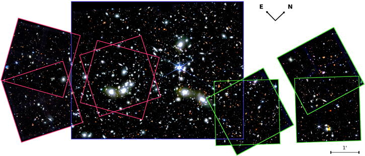
Figure 1. Full view of the color-composite RGB mosaic obtained combining the F090W+F115W+F150W as blue, F200W+F277W as green, and F356W+F410M+F444W as red. The colored boxes show the position of the three different data sets used here: GLASS (green), UNCOVER (blue), and DDT (red). The entire image (including the empty space) is approximately 12 7 × 59 wide.
Download figure:
Standard image High-resolution imageTable 1. NIRCam Exposure Time
| Filter | GLASS1 | GLASS2 | DDT1/2 | UNCOVER1/2/3/4 |
|---|---|---|---|---|
| F090W | 11520 | 16492 | ⋯ | ⋯ |
| F115W | 11520 | 16492 | 2104 | 10823 |
| F150W | 6120 | 8246 | 2104 | 10823 |
| F200W | 5400 | 8246 | 2104 | 6700 |
| F277W | 5400 | 8246 | 2104 | 6700 |
| F356W | 6120 | 8246 | 2104 | 6700 |
| F410M | ⋯ | ⋯ | ⋯ | 6700 |
| F444W | 23400 | 32983 | 2104 | 8246 |
Note. Exposure time (in seconds) for each pointing of the three programs considered here.
Download table as: ASCIITypeset image
As a result of the overlap between programs and of their different observation strategies, such as the different PAs adopted that created multiple star diffraction spikes in the overlapping regions, the resulting exposure map is complex and inhomogenous across bands and area. An analysis of the depth resulting from this exposure map is reported below.
2.2. Data Reduction
2.2.1. Prereduction Steps
Image prereduction was executed using the official JWST calibration pipeline, provided by the Space Telescope Science Institute (STScI) as a Python software suite. 21 We adopted version 1.8.2 (Bushouse et al. 2022) of the pipeline and versions between jwst_1014.pmap and jwst_1019.pmap of the CRDS files (the only change between these versions is the astrometric calibration, which is dealt with as described below). We executed the first two stages of the pipeline (i.e., calwebb_detector1 and calwebb_image2), adopting the optimized parameters for the NIRCam imaging mode, which convert single-detector raw images into photometrically calibrated images.
Using the first pipeline stage calwebb_detector1, we processed the raw uncalibrated data (uncal.fits) in order to apply detector-level corrections performed on a group-by-group basis. These include dark subtractions, reference pixel corrections, nonlinearity corrections, and jump detection, which allows us to identify cosmic-ray (CR) events in the single groups. The last step of this pipeline stage allows us to derive the mean countrate in units of counts per second for each pixel by performing a linear fit to the data in the input image (the so-called ramp-fitting), excluding the group that is masked due to the identification of a CR jump.
The output files of the previous steps (rate.fits) are processed through the second pipeline stage calwebb_image2, which consists of additional instrument-level and observing-mode corrections and calibrations such as the geometric-distortion correction, the flat-fielding, and the photometric calibrations, which convert the data from units of countrate into surface brightness (i.e., megajanskys per steradian) and generate a fully calibrated exposure (cal.fits).
The cal.fits file also contains an rms extension, which combines the contribution of all pixel noise sources, and a DQ mask where the first bit (DO_NOT_USE) identifies pixels that should not be used during the resampling phase.
We then applied a number of custom procedures to remove instrumental defects that are not dealt with the STScI pipeline. Some of them have already been adopted in Merlin et al. (2022, hereafter M22) and are described there: we illustrate below only the main changes to the STScI pipeline in the default configuration and/or to the procedure adopted in M22.
- 1."Snowballs," i.e., circular artifacts observed in the in-flight data caused by a large CR impacts. These hits leave a bright ring-shaped defect in the image because the affected pixels are just partially identified and masked. In M22, we developed a technique to fully mask out these features, which was not necessary here. Indeed, version 1.8.1 of the JWST pipeline introduced the option to identify snowball events, expanding the typical masking area to include all the affected pixels. This new implementation provides the opportunity to correct for these artifacts directly at the ramp-fitting stage, at the cost of a higher noise on the corresponding pixels. We enabled this nondefault option and fine-tuned the corresponding parameters to completely mask all the observed snowballs and at the same time, minimize the size of high-noise areas.
- 2."NL Mask": we find groups of deviant bright pixels on the cal images taken with the NIRCam Module B LW detector, more evident on deeper pointings. They are not well corrected during the prereduction stage and are identified as "WELL_NOT_DEFINED" pixels 22 in the NonLinearity Calibration file. 23 We recognize them by their flag in the DQ and mark them as DO_NOT_USE for the coaddition.
- 3.1/f noise, which introduces random vertical and horizontal stripes in the images (see Schlawin et al. 2020). We removed this by subtracting the median value from each line/column. To remove the flux from objects as accurately as possible, we masked out all objects and the bad pixels flagged in the data quality. The masks were obtained from the segmentation maps obtained with SExtractor (version 2.25.0; Bertin & Arnouts 1996), and then they were further dilated in order to exclude the contamination from the faint outskirt of the objects, which escape detection below the SExtractor threshold. We have applied a differential procedure to dilate objects depending on their ISOAREA: the segmentation of objects with ISOAREA < 5000 pixels was dilated using a 3 × 3 convolution kernel and a dilation of 15 pixels, while for the segmentation of objects with ISOAREA ≥5000 pixels, a 9 × 9 convolution kernel and a dilation of 4 × 15 pixels was used. The procedure was executed separately for each amplifier in the SW detectors (i.e., four times for each individual image) with the exception of the denser areas corresponding to the centers of the clusters and the brightest field star, where objects are significantly larger than the amplifier width (500 pixels, corresponding to about 30'') and could not be masked efficiently. In this case, we removed the 1/f noise over the entire row. Our procedure, which was already adopted in the first release of the GLASS data (M22), is conceptually similar to the one adopted for the CEERS data (Bagley et al. 2022). We publicly release the code adopted for this step.
- 4.Scattered light: we identify additive features in the F115W, F150W, and F200W images. These low-surface brightness features have already been revealed by commissioning data (see Rigby et al. 2023) and are due to scattered light entering the optical path. These anomalies have been dubbed wisps or claws, depending on their origin and morphology. Wisps have a nearly constant shape and can thus be subtracted from the images with simple templates. We removed these features by extracting their 2D profile from the available template (we do not use the entire template image to avoid subtracting its empty but noisy regions) and then normalizing the residual template to match the feature intensity in each image. Claws have first been identified and singled out in images. Their shape in each image has been reconstructed by interpolating a 2D mesh with a box size of 32 pixels and then eventually subtracted from the same image. These procedures efficiently remove most of these features, as shown in Figure 2.We found other defects in the F090W image, and to a lesser extent in the F115W, in images taken in 2022 June. These defects consist of additional scattered light in the images, resulting in artificial sources along the field of view, and they are due to a so-called wing-tilt event, i.e., a small shift of one of the wings of the primary mirror. We adopted the procedure described in M22 to identify and mask these artifacts from images. We emphasize that they do not affect the images taken in 2022 November.
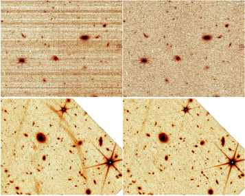
Figure 2. Examples of custom procedures to remove residual instrumental defects that are not dealt with the current STScI pipeline. Top: 1/f stripes removal on a GLASS F200W single exposure. Bottom: portion of the GLASS F150W mosaic before and after the claws treatment.
Download figure:
Standard image High-resolution imageWe then rescaled the single exposures to units of microjanskys per pixel using the conversion factors output by the pipeline.
We also note that our procedure to remove the 1/f noise and the background effectively removes the intracluster light (ICL) from the images. We caution the user to avoid using these images to study the ICL in detail.
2.2.2. Astrometry
The astrometric calibration was performed using SCAMP (Bertin 2006), with third-order distortion corrections. Compared to the procedure we adopted in M22, we started from the distortion coefficient computed by the STScI pipeline, stored in the cal images. We refined the astrometric solution by running scamp in cal mode, which optimizes the solution with limited variations from the starting solution. We have found this procedure both accurate and reliable, as described below. We first obtained a global astrometric solution for the F444W image, which is usually the deepest. As not enough Gaia Data Release 3 (DR3) stars can be used for every NIRCam detector, we have aligned the images to a ground-based catalog obtained in the i-band with the Magellan telescope in good seeing condition (see T22 for details) of the same region, which had been previously aligned to Gaia DR3 stars (Gaia Collaboration 2016). We then took the resulting high-resolution catalog in F444W as reference for the other JWST bands, using compact, isolated sources detected at high signal-to-noise ratio (S/N) at all wavelengths. Each NIRCam detector has been analyzed independently in order to simplify the treatment of distortions and minimize the offsets of the sources in different exposures. Finally, we used SWarp (Bertin et al. 2002) to combine the single exposures into mosaics projected onto a common aligned grid of pixels, and SExtractor to further clean the images by subtracting the residual sky background. The pixel scale of all the images was set to 0031 (the approximate native value of the short-wavelength bands) to allow for simple processing with photometric algorithms.
The final image, computed as a weighted stack of all the images from the three programs, has a size of 24,397 × 21,040 pixels, corresponding to 12.6 × 10.87 arcmin2. In this frame, the area covered by the wide-band NIRCam images (F115W, F150W, F200W, F277W, F356W, and F444W) is exactly 46.5 arcmin2.
Given the especially deep and sharp nature of the JWST images, where most of the faint objects have sizes below 05, the requirements on the final astrometric accuracy are extremely tight to avoid errors in the multiband photometry (where a displacement of as little as 01 can bias the color estimates). These requirements must also be met in the overlapping regions of the various surveys, which have often been observed with different detectors.
To verify the final astrometric solution, we conducted a number of validation tests, where we compare the positions of cross-matched objects in catalogs extracted from different images. For each of these catalogs, we used SExtractor in single-image mode and adopted the XWIN and YWIN estimators of the object center, which are more accurate than other choices. Given the unprecedented image quality of NIRCam, the center of extragalactic objects with complex morphology may be difficult to estimate with high accuracy, particularly when observed across a large wavelength interval. Therefore, we only compared objects with well-defined positions to minimize errors, using the ΔX, ΔY = ERRAWIN_WORLD, and ERRBWIN_WORLD estimators of the error and limited the analysis to objects with  . From these catalogs, we estimated both the average offset of the object centers
  and
and  and the median average deviation madα
and madδ
, which measure the intrinsic scatter in the alignment. In Figure 3 we report the main outcome of these tests:
and the median average deviation madα
and madδ
, which measure the intrinsic scatter in the alignment. In Figure 3 we report the main outcome of these tests:
- 1.We first compared the positions of objects in the original Magellan i-band and the resulting F444W of the entire mosaic (left panel). We find an essentially zero offset and madα ≃ madδ ≃ 002, which is two-thirds of a pixel.
- 2.We compared the F444W catalog with the catalog released by Kokorev et al. (2022) in the context of the ALMA lensing cluster survey (ALCS), containing Hubble Space Telescope (HST) and IRAC sources in the A2744 region (middle-left panel). Overall, the comparison results in a good alignment with a very small offset (
 and ) and madα
≃madδ
≃ 002.
and ) and madα
≃madδ
≃ 002. - 3.We compared the F444W catalog with the AstroDeep H160 catalog obtained on the central region of the A2744 cluster (middle panel), as obtained in the context of the Frontier Fields initiative (Merlin et al. 2016a). While the intrinsic scatter is still good (madα ≃ madδ ≃ 002), we find a systematic offset by about 1 pixel in R.A. and 2.5 pixels in decl., which is most likely due to different choices in the absolute calibration of the ACS/WFC3 data released within the Frontier Fields.
- 4.We compare here the relative calibration of filters at the two extremes of the spectral range, F444W and F115W, where morphological variations and color terms may change the center position and affect the astrometric procedure (middle-right panel). We find again very good alignment with a negligible offset and small madα ≃madδ ≃ 001.
- 5.Finally, we compare the astrometric solutions in the overlapping areas by independently summing the data of the three different programs and checking the accuracy in the overlapping area (right panel). Again, we find a very good alignment with a negligible offset and small madα ≃ madδ ≃ 001.


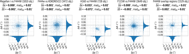
Figure 3. Validation tests of the astrometric registration. The scatter diagrams show the displacement δR. A. and δdecl. of sources between the sources detected in this catalog and those in several reference catalogs. These are on the left, the Magellan i-band catalog registered to Gaia DR3, which is used as global reference for the calibration. On the middle left, the catalog released by Kokorev et al. (2022). In the middle, the AstroDeep catalog on the central region of the A2744 cluster (Merlin et al. 2016a). On the middle right, the catalog of the F115W-detected sources in these images. The right plot shows the objects detected in UNCOVER-only images and those in the GLASS and DDT samples in two overlapping regions. In all diagrams, the average value Δα and Δδ and the median average deviation madΔα and madΔδ are reported.
Download figure:
Standard image High-resolution imageWe adopted a cross-matching radius r = 01 in most of the validation tests, except in the comparison with the AstroDeep catalog, for which we adopted a much larger radius (r = 04), given the larger offset at the level of 0075. We also note that the scatter in δ seems consistently lower than that in α, but we failed to identify a clear origin for this effect, which does not impact the global accuracy. We therefore conclude that the astrometric procedure is accurate and adequate for the goals of this Stage I release. In the future, we plan to explore further and validate other options for astrometric registration and also release images with a smaller pixel scale to better exploit the unprecedented image quality of the JWST data. However, we note that the GLASS-JWST data have a very limited dithering pattern (which was driven by spectroscopic requirements) and so may benefit only marginally from moving to smaller pixels.
2.3. Estimating the Final Depth
The final coaddition of the different images is weighted according to their depth, as estimated by the rms image produced by the pipeline. We therefore obtain an optimally averaged image with the resulting rms image. We verified a posteriori whether the noise estimate encoded in the rms effectively reproduced the photometric noise. To do this, we injected artificial point sources of known magnitude in empty regions of the image and measured their fluxes and uncertainties with a-phot (Merlin et al. 2019), using apertures with a radius of 01. To consider that the mosaics have varying depths resulting from a complex pattern of different exposures, we perfomed this analysis separately over four different image regions that were chosen to have an approximately constant exposure time.
In general, we find that the rms of the resulting flux distribution is 1.1× higher than the value we would expect from the SExtractor errors, computed from the rms image. Furthermore, a larger difference (1.4×) is found for the F444W GLASS image, which is affected by a residual pattern due to poor flat-fielding with the current calibration data. We therefore rescaled the rms maps produced by the pipeline according to these factors.
The resulting depth of this procedure is shown in Figure 4. The rms image is converted into a 5σ limiting flux computed on a circular aperture with a diameter of 02, which is the size adopted to estimate colors of faint sources. The depth ranges from ≃28.6 AB on the DDT2 footprint (in particular, the area that does not overlap with DDT1) to ≃30.2 AB in the area where GLASS1 and GLASS2 overlap, arguably one of the deepest images obtained by JWST so far.
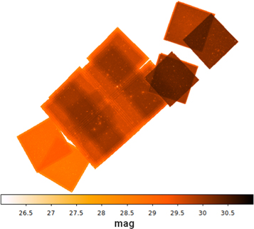
Figure 4. Depth of the full-mosaic F444W image as produced by our pipeline based on the variance image of each exposure and with the renormalization described in the text. Each pixel has been converted into 5σ limiting flux computed on a circular aperture of 02.
Download figure:
Standard image High-resolution imageA more quantitative assessment of the depth in the various filters is reported in Figure 5, where we show the distribution of the limiting magnitudes in each image resulting from the different strategies adopted by the surveys, computed as described above. A clear pattern is seen, illustrating the large, mid-depth area obtained by UNCOVER and the shallower and deeper parts obtained by DDT and GLASS, respectively.
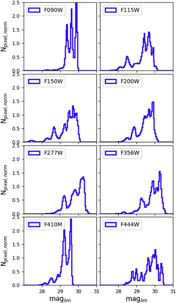
Figure 5. Distribution of the limiting magnitude for each band, as shown in the legend. Limiting magnitudes per pixel are computed as in Figure 4, converting each rms pixel into the corresponding 5σ limiting flux computed on a circular aperture of 02.
Download figure:
Standard image High-resolution image2.4. Hubble Space Telescope Imaging
We have also used the existing images obtained with HST in previous programs, namely, with the F435W, F606W, F775W, and F814W bands with ACS and the F105W, F125W, F140W, and F160W bands with WFC3—other HST data are available from MAST, but are either too shallow and/or limited in area and are not used in our work. These data also include the images that we obtained with DDT Program HST-GO-17231 (PI: Treu), which was specifically aimed at obtaining ACS coverage for the majority of the GLASS1 and GLASS2 fields. We have used calibrated stacked image and weights (G. Brammer, private communication) that we have realigned (after checking that the astrometric solution is consistent) onto our reference grid to allow a straightforward computation of colors.
3. Photometric Catalog
3.1. Detection
We follow here the same prescriptions as were adopted by M22 and Castellano et al. (2022, 2023). We performed source detections on the F444W band because it is generally the deepest or among the deepest image for each data set, and because high-redshift sources (which are the main focus of these observations) are typically brighter at longer wavelengths, where they are observed beyond the Balmer break and in a region that is dominated by emission lines. This approach has the advantage of delivering a clear-cut criterion for the object detections that can easily be translated into a cut of rest-frame properties for high-redshift sources.
We used SExtractor, adopting a double-pass object detection as applied for the HST-CANDELS campaign (see Galametz et al. 2013), to detect the objects following the recipes and parameters described in M22. We note, in particular, that we adopt a detection threshold corresponding to an S/N of 2. This is based on simulations and on the visual inspection of the images at various wavelengths, and has been chosen to maximize the number of detected sources while maintaining the number of spurious ones still limited, as discussed in M22. As in M22, we adopted the following SExtractor parameters: DETECT_MINAREA = 8, DETECT_THRESH = ANALYSIS_THRESH = 0.7071, DEBLEND_NTHRESH = 32, DEBLEND_MINCOUNT = 0.0003, BACK_SIZE = 64, BACK_FILTERSIZE =3, and CLEAN_PARAM = 1, and detection has been performed adopting a Gaussian filter with FWHM = 014.
The final SExtractor catalog of the entire A2744 area contains 24,389 objects.
Estimating the completeness and purity in a noncontiguous (in terms of area and exposure) mosaic derived from the large number of observations adopted here is intrinsically ambiguous. As shown in Figure 5, the depth of these images spans approximately 2 mag, and the completeness is therefore inhomogeneous—not to mention the existence of the cluster, which complicates both the detection and the estimate of the foreground volume (C22b). For these reasons, we do not attempt the traditional estimate of the completeness and refer to Figures 4 and to 5 for an evaluation of the depth. For a proper analysis of the completeness, we refer to the method adopted by C22b, where we estimate the completeness separately on the individual mosaics of the three data sets, which were processed independently. We make the three mosaics available upon request for this purpose.
3.2. Photometry
We have compiled a multiwavelength photometric catalog again following the prescriptions of M22, which in turn is based on previous experience with HST images in CANDELS (see, e.g., Galametz et al. 2013) and in AstroDeep (Merlin et al. 2016a, 2021). The catalog is based on a detection performed on the F444W image described above, and point-spread function (PSF) matched aperture photometry of all the sources. We include all the NIRCam images presented here and existing images obtained with HST in previous programs, namely, with the F435W, F606W, F775W, and F814W bands with ACS and the F105W, F125W, F140W, and F160W bands with WFC3.
The images considered here have PSFs that range from 0035 to 02. Considering that most of the objects have small sizes, with half-light radii smaller than 02, it is necessary to apply a PSF homogenization to avoid bias in the derivation of color across the spectral range.
3.2.1. Point-spread Function Matching
Since the detection band has the coarsest resolution, we performed a PSF match for all the other NIRCam images for color fidelity. We created convolution kernels using the WebbPSF models publicly provided by STScI, 24 combining them with a Wiener filtering algorithm based on the one described in Boucaud et al. (2016). To smooth the images, we used a customized version of the convolution module in t-phot (Merlin et al. 2015, 2016b), which uses FFTW3 libraries. However, we note that this approach cannot fully correct for the inhomogeneities of the PSF: the calibration upon which WebbPSF is calibrated is inevitably initial, and the JWST PSF depends on time and position (Nardiello et al. 2022), and our data set is the inhomogeneous combination of data obtained at different times and with different PAs, so that the PSF definitely changes over the field. For this version of the catalog, we used the UNCOVER PSF models (epoch: 2022/11/07, PA: 41.2 deg) as average PSFs, and we plan to improve our PSF estimation in future versions of the catalog that will be released in Stage II.
Similarly, concerning the HST images, we note that all of them have too few stars to obtain a robust estimate of the PSF directly from the images, so we adopt in all cases existing HST PSFs that were taken from CANDELS. This approximation may introduce small biases in the final catalog. ACS images have been PSF-matched to F444W, while for the WFC3 F105W, F125W, F140W, and F160W images, which have a PSF larger than that of F444W, we have done the inverse, that is, we smoothed the F444W image and the WFC3 F105W, F125W, and F140W to the F160W and followed a slightly different procedure that we describe below.
3.2.2. Flux Estimate
The total flux is measured with a-phot on the detection image F444W by means of a Kron elliptical aperture (Kron 1980). As we have shown in M22, simulations suggest that Kron fluxes measured with a-phot are are somewhat less affected by systematic errors, while being slightly more noisy.
Then, we used a-phot to measure the fluxes at the positions of the detected sources on the PSF-matched images, masking neighboring objects using the SExtractor segmentation map. Given the wide range of magnitudes and sizes of the target galaxies, we measured the flux in a range of apertures: the segmentation area (the images being on the same grid and PSF-matched) and five circular apertures with diameters that are integer multiples (2, 3, 8, and 16 times) of the FWHM in the F444W band, which correspond to 028, 042, 112, and 224 diameters. For the four WFC3 images (which have a PSF larger than that of F444W), we first filtered the F444W to their FWHM and then measured the colors between the filtered F444W and the WFC3 images. To minimize biases when these colors are combined with those of the other bands, we use in this case apertures the same multiples of the WFC3 PSF adopted for the other bands. We remark that this procedure is only approximate and delivers a first-order correction of the systematic effects due to different PSFs. In a future release, we plan to adopt more sophisticated approaches to optimize the photometry, including but not limited to the improvement of the PSF estimate and applying t-phot on WFC3 images that have a larger PSF.
Total fluxes are obtained in the other bands by normalizing the colors in a given aperture to the F444W total flux, i.e., by computing fm,total = fm,aper/fF444W,aper × fF444W,total, as described in M22.
We release the five catalogs described above (one computed on segmentation, and four computed on the different apertures), and we leave it to the user to choose the most suitable catalog for a given science application. In general, small-aperture catalogs are more appropriate for faint sources as they match their small sizes and minimize the effect of contamination from nearby sources, which can be high for blended objects. Larger apertures may be more appropriate for brighter sources and especially cluster members.
3.2.3. Validation Tests
We have performed a few validation tests to primarily verify the flux calibration, which has been the subject of many revisions in these first months, and to a lesser extent, the procedure adopted to derive the photometric catalog.
The overlap between the southern quadrants in GLASS1 and GLASS2 offers a nice opportunity to test the NIRCam flux calibration. Indeed, the two GLASS observations have been observed in two epochs (2022 June and November) with a PA difference of nearly 150°. As a result, the southern quadrants of GLASS1 and GLASS2 largely overlap, but have been observed with modules B and A, respectively. We therefore obtained stacked images of the two epochs separately, built a photometric catalog with the same recipes, and checked the magnitude difference between objects observed with different detectors. The result of this exercise, done on all bands, is reported in Figure 6. We note that in the short bands, the two modules are made of four detectors, each with an independent calibration, which we plot all together in Figure 6. The comparison, that is, limited to objects observed with high S/N > 25, shows that the average magnitude difference between the two modules is in general quite small, and is below 0.05 mag in all cases (see Figure 6 and its captions for details). This confirms that the flux calibration between the different modules is reasonably stable at this stage.
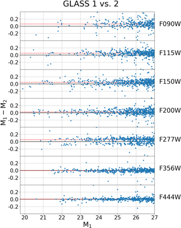
Figure 6. Stability of the photometric calibration between different detectors as measured by comparing the photometry of high S/N objects (S/N > 25) detected in the two epochs of observations in the SE quadrant of GLASS (lower-leftmost green square in Figure 1). Objects in this area have been observed in two epochs (2022 June and November) and with modules B and A, respectively. For each filter, the difference in magnitude ΔM = M1 − M2 for objects between epoch1 and epoch2 as a function of M1 is reported. The dashed red lines represent the median offsets. We found  with mad ≈ 0.05 for F090W,
  with mad ≈ 0.04 for F115W,
  with mad ≈ 0.04 for F150W,
  with mad ≈ 0.04 for F200W,
  with mad ≈ 0.04 for F277W, and negligible in F356W and F444W with mad ≈ 0.03 and mad ≈ 0.02, respectively. We have visually inspected the bright objects with ∣ΔM∣ > 0.05 and verified that they mostly originate from saturated stars or objects with incomplete coverage.
Download figure:
Standard image High-resolution imageAs a further check to validate the photometric pipeline, we compared the colors of the sources in the region of the A2744 cluster with those measured for the Frontier Fields survey (Lotz et al. 2014) within the AstroDeep project (Merlin et al. 2016a; Castellano et al. 2016). We chose to compare the colors of sources to avoid possible systematics deriving from the total flux estimates obtained on two different bands in the two catalogs; some residual offsets and trends can be due to the different segmented areas. The cross match was performed by selecting objects having mH160 < 24, assuming a positional accuracy Δr < 04 to account for the possible mismatch in absolute astrometry between the two. This comparison is shown in Figure 7, where we show isophotal colors computed on PSF-matched images as a function of the H160 magnitude of the Astrodeep catalog, also providing running and global median offsets. We note that in Merlin et al. (2016a), we explicitly modeled and subtracted the ICL and the brightest cluster sources. This was especially needed to derive accurate colors on Spitzer images, which have a much poorer resolution. In this case, our procedure to remove the 1/f noise, and the background effectively removes a significant fraction of the ICL, to the point that objects falling in these areas do not show any systematic shift of the objects in Figure 7. Therefore, the removal of the brightest cluster members is postponed to the release of Stage II. We also note that for the same reason, our images are not adequate for studying the ICL emission. The comparison shows that when the same approach is used to estimate colors, i.e., isophotal magnitudes are adopted, the agreement between the two catalogs is good (although the shallowness and low resolution of the IRAC bands makes the comparison less accurate).
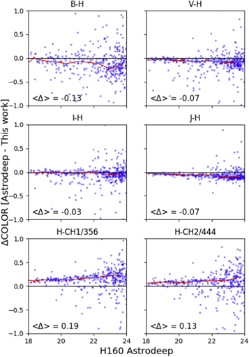
Figure 7. Comparison between the colors measured in six bands from this catalog and from the Astrodeep catalog (Merlin et al. 2016b). Each panel shows the difference in a color as a function of the H160 magnitude from the Astrodeep catalog. The red lines show the running medians, and their weighted averages are also given.
Download figure:
Standard image High-resolution imageFrom this comparison, we conclude that—quite reassuringly—the overall photometric chain is consistent between the well-established Frontier Fields data and these new data. At the same time, we remark that the optimal choice of the aperture depends on the size and type of object under study. Small apertures tend to have higher S/N and should be preferred for faint sources. For the brightest sources, larger apertures should be preferred. It is also possible to estimate rough color gradients by comparing the various apertures that we release. We also tested that applying the same technique without PSF matching introduces an offset of ∼0.2 mag in the final colors, which would clearly affect the derived photometric redshifts and spectral engery distribution fitting results.
Finally, in an effort to cross-validate our results prior to release, in the leadup to this paper, we compared our catalogs to those under development by the UNCOVER team (Weaver et al. 2023, in preparation) based on the same raw data sets. The image-processing and photometric procedures adopted by the two teams have significant differences. The main differences are (i) the image coaddition (the UNCOVER team adopts Grizli from Brammer 2019, while we use a custom pipeline that uses scamp and swarp); (ii) the object detection (UNCOVER uses an optimally stacked F277W+F356W+F444W image after removing the ICL, while we use F444W); and (iii) techniques and tools for PSF matching and photometry. For these reasons, we found some differences between the catalogs, especially for faint sources at the detection limit, as expected. However, our comparison of working versions of the catalogs produced by the two teams shows a good agreement in the colors and magnitudes of the vast majority of objects overall, as shown in Figure 8 in the Appendix.
4. Summary
We present the data obtained by three NIRCam programs on the A2744 cluster in this paper: the GLASS-JWST Early Release Science Program, UNCOVER, and the Directory Discretionary Time 2756. All the data, taken with eight different filters (F090W, F115W, F150W, F200W, F277W, F356W, F410M, and F444W), have been reduced with an updated pipeline that builds upon the official STScI pipeline, but includes a number of improvements to better remove some instrumental signature and to streamline the process.
All frames have been aligned onto a common frame with a 0031 pixel scale, approximately matching the native pixel scale of the short-wavelength data. The final images of the whole A2744 region cover an area of 46.5 arcmin2 with a PSF ranging from 0035 (for the F090W image) to 014 (F444W), and reach astonishingly deep 5σ magnitude limits from 28.5 to 30.5, depending on the location and filter.
We also exploit other HST publicly available programs that have targeted the area, including also the available HST ACS and WFC3 data in the F435W, F606W, F775W, and F814W (ACS) and F105W, F125W, F140W, and F160W (WFC3) bands, to expand the coverage of the visible-to-IR wavelength range.
We derive a photometric catalog from these data by detecting objects in the F444W image and computing PSF-matched forced photometry on the remaining bands.
We made several tests to validate the photometric calibrations, either internal, based on overlapping parts observed in different epochs with different modules, or external, based on the cross-correlation with the AstroDeep catalog of the cluster region. They both confirm that photometric offset are limited to 0.05 mag at most. Slightly larger (0.1 mag) systematic biases, especially when HST bands are concerned, could be due to the simplified PSF matching we adopt in this first release.
We remark again that we did not explicitly remove the ICL. However, our procedure to remove the 1/f noise and the background on scales larger than the larger detected object are effective also in removing the ICL from the images. We therefore tested that the photometry is not significantly affected. Needless to say, this makes this data set unfit for studying the ICL, and we caution against using this data set for this purpose. We also note that we did not model and subtract the brightest galaxy members, which is at variance with what we did in Merlin et al. (2016a), so that the photometry of objects falling on their outskirts can be severely contaminated and made brighter and generally redder.
We publicly release the entire mosaic of the NIRCam images. The three individual images of each program, which are more homogeneous in terms of PSF orientation and coverage/depth and potentially are more suitable for accurate photometry and for accurate estimate of incompleteness, are also available upon request.
We also publicly release the multiwavelength catalog of the entire A2744 area, which includes 24,389 objects. We release five independent catalogs, based on a different aperture (namely, 028, 056, 112, and 224, corresponding to 2, 3, 8, and 16 times the PSF of the F444W image) and in the isophotal area. This catalog is optimized for high-redshift galaxies, and in general, for faint extragalactic sources, and it is aimed at allowing a first look at the data and the selection of targets for Cycle 2 proposals. In future releases, we plan to include updated calibrations and procedures for the image processing, and we plan to optimize the photometry with more sophisticated approaches for PSF matching.
Finally, we also release the code we developed to remove the 1/f noise from the NIRCam images, which improves the current implementation in the STScI pipeline with a more effective masking of sources in the image.
Images, catalogs, and software are immediately available for download from the GLASS-ERS collaboration 25 and AstroDeep website. 26 They will also be made available at the MAST archive upon acceptance of the paper.
All the JWST data used in this paper can be found in MAST:10.17909/kw3c-n857.
Acknowledgments
We warmly thank J. Weaver, K. Whitaker, I. Labbé, and R. Bezanson for sharing their data with us prior to publication, which made it possible to compare the two processes for data analysis. This work is based on observations made with the NASA/ESA/CSA James Webb Space Telescope, and with the NASA/ESA Hubble Space Telescope. The data were obtained from the Mikulski Archive for Space Telescopes at the Space Telescope Science Institute, which is operated by the Association of Universities for Research in Astronomy, Inc., under NASA contract NAS 5-03127 for JWST and NAS 526555 for HST. These observations are associated with program JWST-ERS-1324, JWST-DDT-2756, and JWST-GO-2561, and several HST programs. We acknowledge financial support from NASA through grant JWST-ERS-1324. This research is supported in part by the Australian Research Council Centre of Excellence for All Sky Astrophysics in 3 Dimensions (ASTRO 3D) through project number CE170100013. K.G. and T.N. acknowledge support from Australian Research Council Laureate Fellowship FL180100060. M.B. acknowledges support from the Slovenian national research agency ARRS through grant No. N1-0238. We acknowledge financial support through grant Nos. PRIN-MIUR 2017WSCC32 and 2020SKSTHZ. We acknowledge support from the INAF Large Grant 2022 "Extragalactic Surveys with JWST" (PI: Pentericci). C.M. acknowledges support by the VILLUM FONDEN under grant No. 37459. R.A.W. acknowledges support from NASA JWST Interdisciplinary Scientist grant Nos. NAG5-12460, NNX14AN10G, and 80NSSC18K0200 from GSFC. The Cosmic Dawn Center (DAWN) is funded by the Danish National Research Foundation under grant DNRF140. This work has made use of data from the European Space Agency (ESA) mission Gaia (https://www.cosmos.esa.int/gaia), processed by the Gaia Data Processing and Analysis Consortium (DPAC,https://www.cosmos.esa.int/web/gaia/dpac/consortium). Funding for the DPAC has been provided by national institutions, in particular, the institutions participating in the Gaia Multilateral Agreement. The authors thank Paola Marrese and Silvia Marinoni (Space Science Data Center, Italian Space Agency) for their contribution to the work.
Software: astropy (Astropy Collaboration et al. 2013, 2018, 2022), a-phot (Merlin et al. 2019), denoise_nircam (https://github.com/diegoparis10/denoise_NIRCam), Grizli (Brammer 2019), matplotlib (Hunter 2007), numpy (Van der Walt et al. 2011), SCAMP (Bertin 2006), SExtractor (Bertin & Arnouts 1996), JWST STScI Calibration Pipeline (Bushouse et al. 2022), SWarp (Bertin et al. 2002), t-phot (Merlin et al. 2015, 2016b), WebbPSF (Perrin et al. 2012, 2014).
Appendix
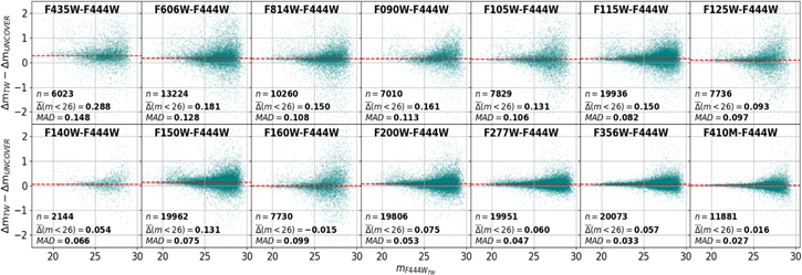
Figure 8 shows the color comparison between our catalog and the catalog released by the UNCOVER collaboration (Weaver et al. 2023) on the same data set, for which we take the final released version. The two catalogs have been obtained with largely independent procedures for data reduction, source detection, PSF homogenization, and photometry. In addition to the minor differences in the pipelines, for which we refer to Weaver et al. (2023), we explicitly remark that their procedure has explicitly removed ICL and brightest cluster members and adopted different recipes to estimate the PSF. Despite these differences, we find a general good agreement between the two catalogs, in particular for the JWST long wavelength, but also for most of the other bands. There seems to be a systematic trends of our catalog yielding redder colors at shorter bands. We explicitly note that disagreements of the same degree—often even larger—are found when comparing catalogs extracted from previous HST surveys, even though processing of HST data is certainly more established and accurate than that of JWST data, which is due to the lack of complete calibration. While it is tempting to associate these deviations with different PSF-matching techniques, we plan to investigate them in more detail in our final analysis of these data.
Figure 8. Comparison of the colors between this work (TW) and the UNCOVER catalog.  represents the median offset between ΔmTW and ΔmUNCOVER computed by only selecting objects brighter than m = 26 and applying a MAD clipping to the sampled data.
Download figure:
Standard image High-resolution image
Footnotes
- 21
- 22
- 23
- 24
- 25
- 26