Metric and Relative Monocular Depth Estimation: An Overview. Fine-Tuning Depth Anything V2 👐 📚

Evolution of Models

Over the past decade, monocular depth estimation models have undergone remarkable advancements. Let's take a visual journey through this evolution.

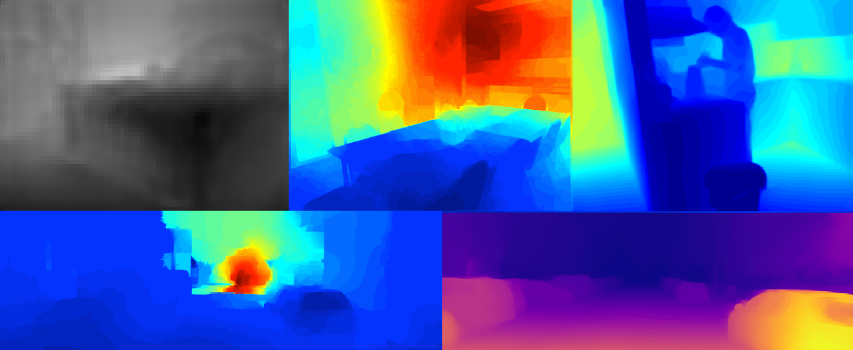
We started with basic models like this:

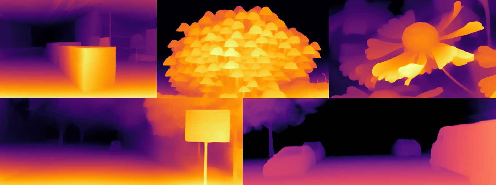
Progressed to more sophisticated models:

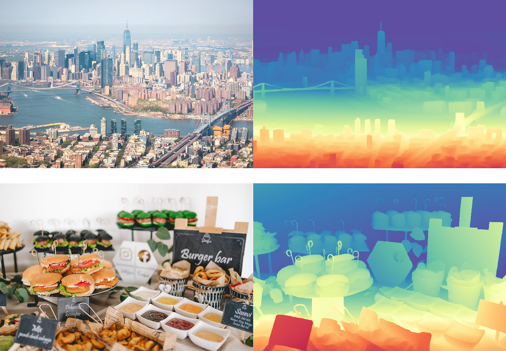
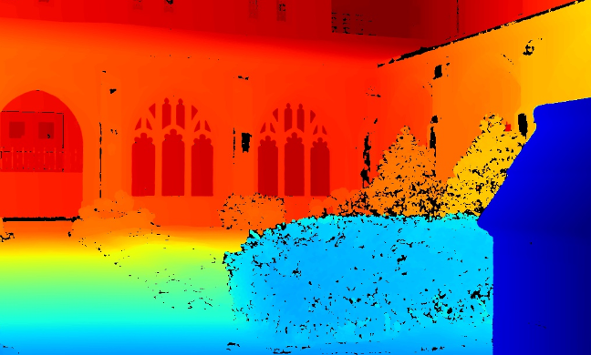
And now, we have the state-of-the-art model, Depth Anything V2:

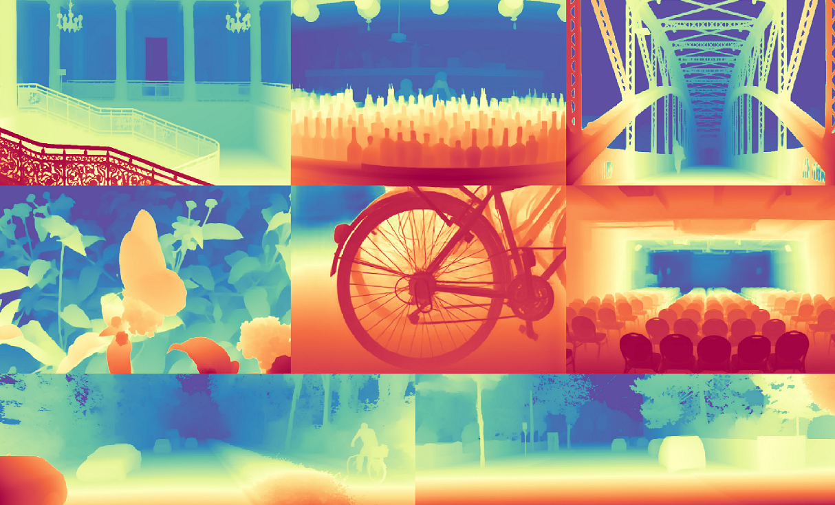
Impressive, isn't it?

Today, we will demystify how these models work and simplify complex concepts. Moreover, we will fine-tune our own model using a custom dataset. "But wait," you might ask, "why would we need to fine-tune a model on our own dataset when the latest model performs so well in any environment?"

This is where the nuances and specifics come into play, which is precisely the focus of this article. If you're eager to explore the intricacies of monocular depth estimation, keep reading.

The Basics

"Okay, what exactly is depth?" Typically, it's a single-channel image where each pixel represents the distance from the camera or sensor to a point in space corresponding to that pixel. However, it turns out that these distances can be absolute or relative — what a twist!

• Absolute Depth: Each pixel value directly corresponds to a physical distance (e.g., in meters or centimeters).
• Relative Depth: The pixel values indicate which points are closer or further away without referencing real-world units of measurement. Often the relative depth is inverted, i.e. the smaller the number, the farther the point is.

We'll explore these concepts in more detail a bit later.

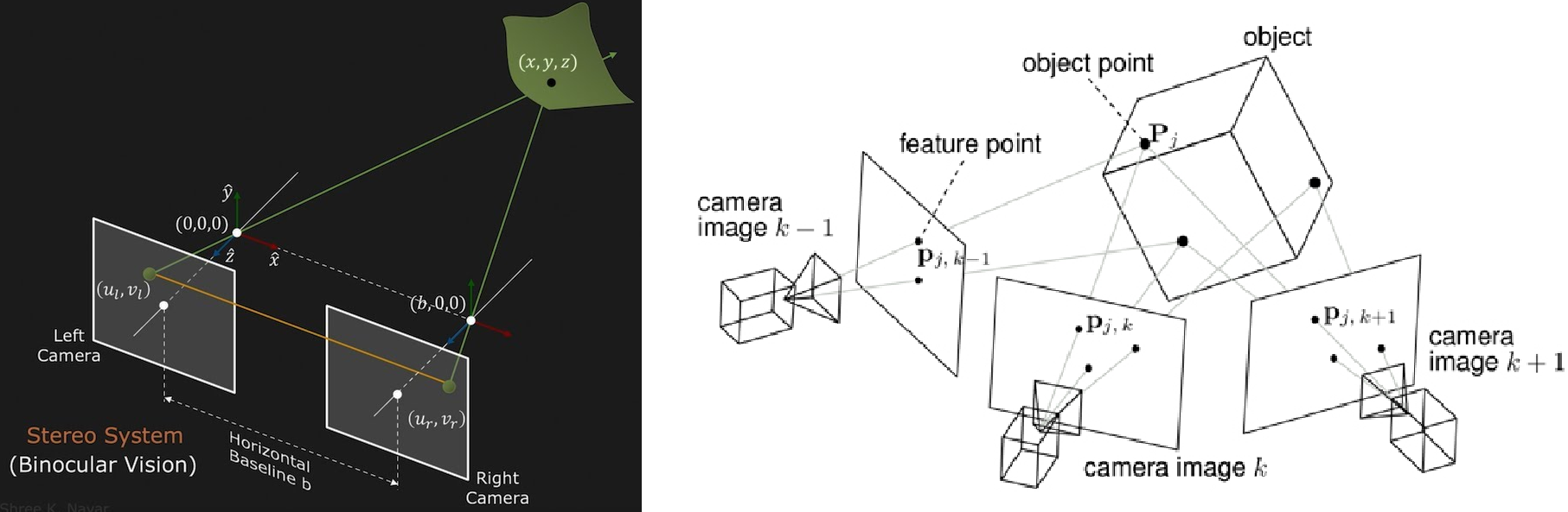
"Well, but what does monocular mean?" It simply means that we need to estimate depth using just a single photo. What’s so challenging about that? Take a look at this:

As you can see, projecting a 3D space onto a 2D plane can create ambiguity due to perspective. To address this, there are precise mathematical methods for depth estimation using multiple images, such as Stereo Vision, Structure from Motion, and the broader field of Photogrammetry. Additionally, technologies like laser scanners (e.g., LiDAR) can be used for depth measurement.

Relative and Absolute (aka Metric) Depth Estimation: What's the Point?

Let's explore some challenges that highlight the necessity of relative depth estimation. And to be more scientific, let's refer to some papers.

The advantage of predicting metric depth is the practical utility for many downstream applications in computer vision and robotics, such as mapping, planning, navigation, object recognition, 3D reconstruction, and image editing. However, training a single metric depth estimation model across multiple datasets often deteriorates the performance, especially when the collection includes images with large differences in depth scale, e.g. indoor and outdoor images. As a result, current MDE models usually overfit to specific datasets and do not generalize well to other datasets.

Typically, the architecture for this image-to-image task is an encoder-decoder model, like a U-Net, with various modifications. Formally, this is a pixel-wise regression problem. Imagine how challenging it is for a neural network to accurately predict distances for each pixel, ranging from a few meters to several hundred meters.
This brings us to the idea of moving away from a universal model that predicts exact distances in all scenarios. Instead, let's develop a model that approximately (relatively) predicts depth, capturing the shape and structure of the scene by indicating which objects are farther and which are closer relative to each other and to us. If precise distances are needed, we can fine-tune this relative model on a specific dataset, leveraging its existing understanding of the task.

The problems don't end there

The model not only has to handle images taken with different cameras and camera settings but also has to learn to adjust for the large variations in the overall scale of the scenes.

Apart from different scales, as we mentioned earlier, a significant problem lies in the cameras themselves, which can have vastly different perspectives of the world.

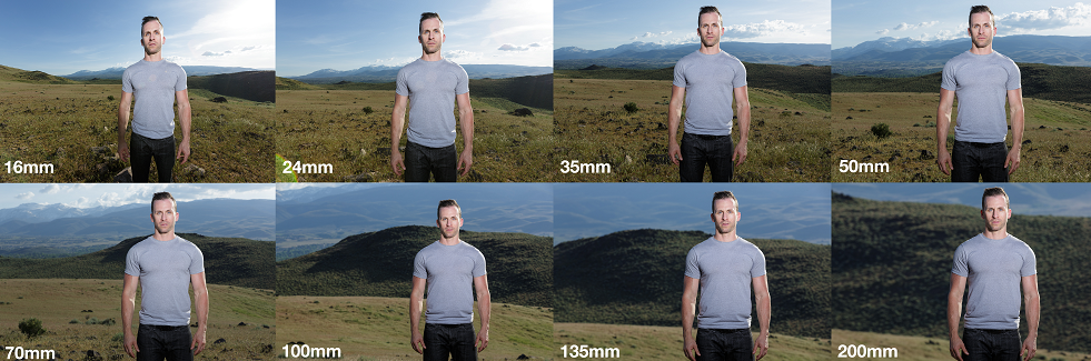
Notice how changes in focal length dramatically alter the perception of background distances!

Lastly, many datasets lack absolute depth maps altogether and only have relative ones (for instance, due to the lack of camera calibration). Additionally, each method of obtaining depth has its own advantages, disadvantages, biases, and problems.

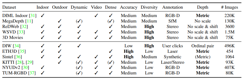
We identify three major challenges. 1) Inherently different representations of depth: direct vs. inverse depth representations. 2) Scale ambiguity: for some data sources, depth is only given up to an unknown scale. 3) Shift ambiguity: some datasets provide disparity only up to an unknown scale and global disparity shift that is a function of the unknown baseline and a horizontal shift of the principal points due to post-processing

In short, I hope I've convinced you that you can't just take scattered depth maps from the internet and train a model with them using some pixel-wise MSE.

But how do we equalize all these variations? How can we abstract as much as possible from the differences and extract commonalities from all these datasets — namely, the shape and structure of the scene, the proportional relationships between objects, indicating what is closer and what is farther away?

Scale and Shift Invariant Loss 😎

Simply put, we need to perform some sort of normalization on all the depth maps we want to train on and evaluate metrics with. We have an idea: we want to create a loss function that doesn't consider the scale of the environment or the various shifts. The remaining task is to translate this idea into mathematical terms.

Concretely, the depth value is first transformed into the disparity space by $d=\frac{1}{t}d\; =\; \backslash frac\{1\}\{t\}$ and then normalized to $0\sim 10\; \backslash sim\; 1$ on each depth map. To enable multi-dataset joint training, we adopt the affine-invariant loss to ignore the unknown scale and shift of each sample: $${\mathcal{L}}_1=\frac{1}{HW}\sum _{i=1}^{HW}\rho (d_i^{\ast },d_i),\backslash mathcal\{L\}\_1\; =\; \backslash frac\{1\}\{HW\}\; \backslash sum\_\{i=1\}^\{HW\}\; \backslash rho(d\_i^*,\; d\_i),$$ where $d_i^{\ast }d\_i^*$ and $d_{i}d\_i$ are the prediction and ground truth, respectively. And $\rho \backslash rho$ is the affine-invariant mean absolute error loss: $\rho (d_i^{\ast },d_i)=\mid {\widehat{d}}_i^{\ast }-{\widehat{d}}_i\mid \backslash rho(d\_i^*,\; d\_i)\; =\; \backslash left|\; \backslash hat\{d\}\_i^*\; -\; \backslash hat\{d\}\_i\; \backslash right|$, where ${\widehat{d}}_i^{\ast }\backslash hat\{d\}\_i^*$ and ${\widehat{d}}_i\backslash hat\{d\}\_i$ are the scaled and shifted versions of the prediction $d_i^{\ast }d\_i^*$ and ground truth $d_{i}d\_i$: $${\widehat{d}}_i=\frac{d_i-t(d)}{s(d)},\backslash hat\{d\}\_i\; =\; \backslash frac\{d\_i\; -\; t(d)\}\{s(d)\},$$ where $t(d)t(d)$ and $s(d)s(d)$ are used to align the prediction and ground truth to have zero translation and unit scale: $$t(d)=\mathrm{m}\mathrm{e}\mathrm{d}\mathrm{i}\mathrm{a}\mathrm{n}(d),s(d)=\frac{1}{HW}\sum _{i=1}^{HW}\mid d_i-t(d)\mid \mathrm{.}t(d)\; =\; \backslash mathrm\{median\}(d),\; \backslash quad\; s(d)\; =\; \backslash frac\{1\}\{HW\}\; \backslash sum\_\{i=1\}^\{HW\}\; \backslash left|\; d\_i\; -\; t(d)\; \backslash right|.$$

In fact, there are many other methods and functions that help eliminate scale and shifts. There are also different additions to loss functions, such as gradient loss, which focuses not on the pixel values themselves but on how quickly they change (hence the name — gradient). You can read more about this in the MiDaS paper, i'll include a list of useful literature at the end. Let's briefly discuss metrics before moving on to the most exciting part — fine-tuning on absolute depth using a custom dataset.

Metrics

In depth estimation, several standard metrics are used to evaluate performance, including MAE (Mean Absolute Error), RMSE (Root Mean Square Error), and their logarithmic variations to smooth out large gaps in distance. Additionally, consider the following:

• Absolute Relative Error (AbsRel): This metric is similar to MAE but expressed in percentage terms, measuring how much the predicted distances differ from the true ones on average in percentage terms.
  $\text{AbsRel}=\frac{1}{N}{\sum }_{i=1}^N\frac{\mathrm{\mid }{d}_i-{\widehat{d}}_i\mathrm{\mid }}{d_i}\backslash text\{AbsRel\}\; =\; \backslash frac\{1\}\{N\}\; \backslash sum\_\{i=1\}^\{N\}\; \backslash frac\{|d\_i\; -\; \backslash hat\{d\}\_i|\}\{d\_i\}$
• Threshold Accuracy ( ${\delta }_1\backslash delta\_1$): This measures the percentage of predicted pixels that differ from the true pixels by no more than 25%.
  

Important Considerations

For all our models and baselines, we align predictions and ground truth in scale and shift for each image before measuring errors.

Indeed, if we are training to predict relative depth but want to measure quality on a dataset with absolute values, and we are not interested in fine-tuning on this dataset or in the absolute values, we can, similar to the loss function, exclude scale and shift from the calculations and standardize everything to a unified measure.

Four Methods of Calculating Metrics

Understanding these methods helps avoid confusion when analyzing metrics in papers:

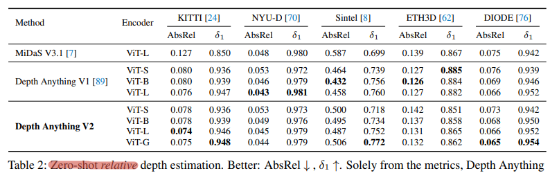
1. Zero-shot Relative Depth Estimation
   • Train to predict relative depth on one set of datasets and measure quality on others. Since the depth is relative, significantly different scales are not a concern, and metrics on other datasets usually remain high, similar to the test sets of the training datasets.

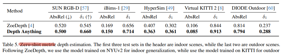
2. Zero-shot Absolute Depth Estimation
   • Train a universal relative model, then fine-tune it on a good dataset for predicting absolute depth, and measure the quality of absolute depth predictions on a different dataset. Metrics in this case tend to be worse compared to the previous method, highlighting the challenge of predicting absolute depth well across different environments.

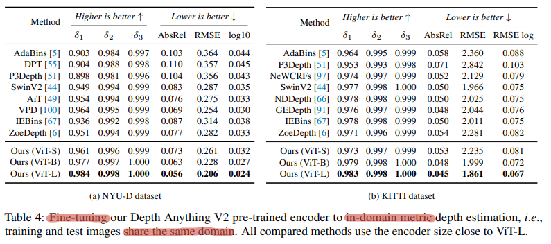
3. Fine-tuned (In-domain) Absolute Depth Estimation
   • Similar to the previous method, but now measure quality on the test set of the dataset used for fine-tuning absolute depth prediction. This is one of the most practical approaches.

4. Fine-tuned (In-domain) Relative Depth Estimation
   • Train to predict relative depth and measure quality on the test set of the training datasets. This might not be the most precise name, but the idea is straightforward.

Depth Anything V2 Absolute Depth Estimation Fine-Tuning

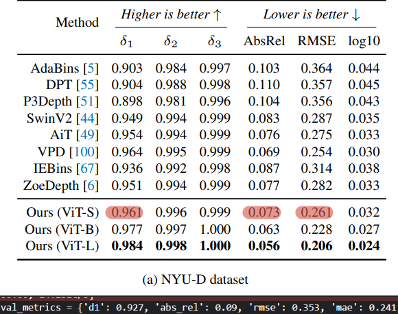
In this section, we will reproduce the results from the Depth Anything V2 paper by fine-tuning the model to predict absolute depth on the NYU-D dataset, aiming to achieve metrics similar to those shown in the last table from the previous section.

Key Ideas Behind Depth Anything V2

Depth Anything V2 is a powerful model for depth estimation, achieving remarkable results due to several innovative concepts:

• Universal Training Method on Heterogeneous Data: This method, introduced in the MiDaS 2020 paper, enables robust training across various types of datasets.
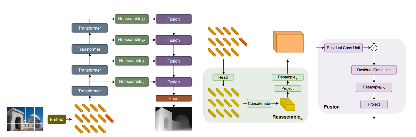
• DPT Architecture: The "Vision Transformers for Dense Prediction" paper presents this architecture, which is essentially a U-Net with a Vision Transformer (ViT) encoder and several modifications.

• DINOv2 Encoder: This standard ViT, pre-trained using a self-supervised method on a massive dataset, serves as a powerful and versatile feature extractor. In recent years, CV researchers have aimed to create foundation models similar to GPT and BERT in NLP, and DINOv2 is a significant step in that direction.
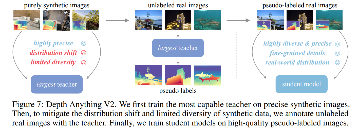
• Use of Synthetic Data: The training pipeline is very well described in the image below. This approach allowed the authors to achieve such clarity and accuracy in the depth maps. After all, if you think about it, the labels obtained from synthetic data are truly “ground truth.”

Getting Started with Fine-Tuning

Now, let's dive into the code. If you don't have access to a powerful GPU, I highly recommend using Kaggle over Colab. Kaggle offers several advantages:

• Up to 30 hours of GPU usage per week
• No connection interruptions
• Very fast and convenient access to datasets
• The ability to use two GPUs simultaneously in one of the configurations, which will help you practice distributed training

You can jump straight into the code using this notebook on Kaggle.

We'll go through everything in detail here. To start, let's download all the necessary modules from the authors' repository and the checkpoint of the smallest model with the ViT-S encoder.

Step 1: Clone the Repository and Download Pre-trained Weights

!git clone https://github.com/DepthAnything/Depth-Anything-V2
!wget -O depth_anything_v2_vits.pth https://huggingface.co/depth-anything/Depth-Anything-V2-Small/resolve/main/depth_anything_v2_vits.pth?download=true

If you don't work at Kaggle, you can download the dataset here

Step 2: Import Required Modules

import numpy as np
import matplotlib.pyplot as plt
import os
from tqdm import tqdm
import cv2
import random
import h5py

import sys
sys.path.append('/kaggle/working/Depth-Anything-V2/metric_depth')

from accelerate import Accelerator
from accelerate.utils import set_seed
from accelerate import notebook_launcher
from accelerate import DistributedDataParallelKwargs

import transformers

import torch
import torchvision
from torchvision.transforms import v2
from torchvision.transforms import Compose
import torch.nn.functional as F
import albumentations as A

from depth_anything_v2.dpt import DepthAnythingV2
from util.loss import SiLogLoss
from dataset.transform import Resize, NormalizeImage, PrepareForNet, Crop

Step 3: Get All File Paths for Training and Validation

def get_all_files(directory):
    all_files = []
    for root, dirs, files in os.walk(directory):
        for file in files:
            all_files.append(os.path.join(root, file))
    return all_files


train_paths = get_all_files('/kaggle/input/nyu-depth-dataset-v2/nyudepthv2/train')
val_paths = get_all_files('/kaggle/input/nyu-depth-dataset-v2/nyudepthv2/val')

Step 4: Define the PyTorch Dataset

#NYU Depth V2 40k. Original NYU is 400k
class NYU(torch.utils.data.Dataset):
    def __init__(self, paths, mode, size=(518, 518)):
        
        self.mode = mode #train or val
        self.size = size
        self.paths = paths
        
        net_w, net_h = size
        #author's transforms
        self.transform = Compose([
            Resize(
                width=net_w,
                height=net_h,
                resize_target=True if mode == 'train' else False,
                keep_aspect_ratio=True,
                ensure_multiple_of=14,
                resize_method='lower_bound',
                image_interpolation_method=cv2.INTER_CUBIC,
            ),
            NormalizeImage(mean=[0.485, 0.456, 0.406], std=[0.229, 0.224, 0.225]),
            PrepareForNet(),
        ] + ([Crop(size[0])] if self.mode == 'train' else []))
        
        # only horizontal flip in the paper
        self.augs = A.Compose([
            A.HorizontalFlip(),
            A.ColorJitter(hue = 0.1, contrast=0.1, brightness=0.1, saturation=0.1),
            A.GaussNoise(var_limit=25),
        ])
    
    def __getitem__(self, item):
        path = self.paths[item]
        image, depth = self.h5_loader(path)
        
        if self.mode == 'train':
            augmented = self.augs(image=image, mask = depth)
            image = augmented["image"] / 255.0
            depth = augmented['mask']
        else:
            image = image / 255.0
          
        sample = self.transform({'image': image, 'depth': depth})

        sample['image'] = torch.from_numpy(sample['image'])
        sample['depth'] = torch.from_numpy(sample['depth'])
        
        # sometimes there are masks for valid depths in datasets because of noise e.t.c
#         sample['valid_mask'] = ... 
     
        return sample

    def __len__(self):
        return len(self.paths)
    
    def h5_loader(self, path):
        h5f = h5py.File(path, "r")
        rgb = np.array(h5f['rgb'])
        rgb = np.transpose(rgb, (1, 2, 0))
        depth = np.array(h5f['depth'])
        return rgb, depth

Here are a few points to note:

• The original NYU-D dataset contains 407k samples, but we are using a subset of 40k. This will slightly impact the final model quality.
• The authors of the paper used only horizontal flips for data augmentation.
• Occasionally, some points in the depth maps may not be processed correctly, resulting in "bad pixels". Some datasets include a mask that differentiates between valid and invalid pixels in addition to the image and depth map. This mask is necessary to exclude bad pixels from loss and metric calculations.

• During training, we resize images so that the smaller side is 518 pixels and then crop them. For validation, we do not crop or resize the depth maps. Instead, we upsample the predicted depth maps and compute metrics at the original resolution.

Step 5: Data Visualization

num_images = 5

fig, axes = plt.subplots(num_images, 2, figsize=(10, 5 * num_images))

train_set = NYU(train_paths, mode='train') 

for i in range(num_images):
    sample = train_set[i*1000]
    img, depth = sample['image'].numpy(), sample['depth'].numpy()

    mean = np.array([0.485, 0.456, 0.406]).reshape((3, 1, 1))
    std = np.array([0.229, 0.224, 0.225]).reshape((3, 1, 1))
    img = img*std+mean

    axes[i, 0].imshow(np.transpose(img, (1,2,0)))
    axes[i, 0].set_title('Image')
    axes[i, 0].axis('off')

    im1 = axes[i, 1].imshow(depth, cmap='viridis', vmin=0)
    axes[i, 1].set_title('True Depth')
    axes[i, 1].axis('off')
    fig.colorbar(im1, ax=axes[i, 1])
    
plt.tight_layout()

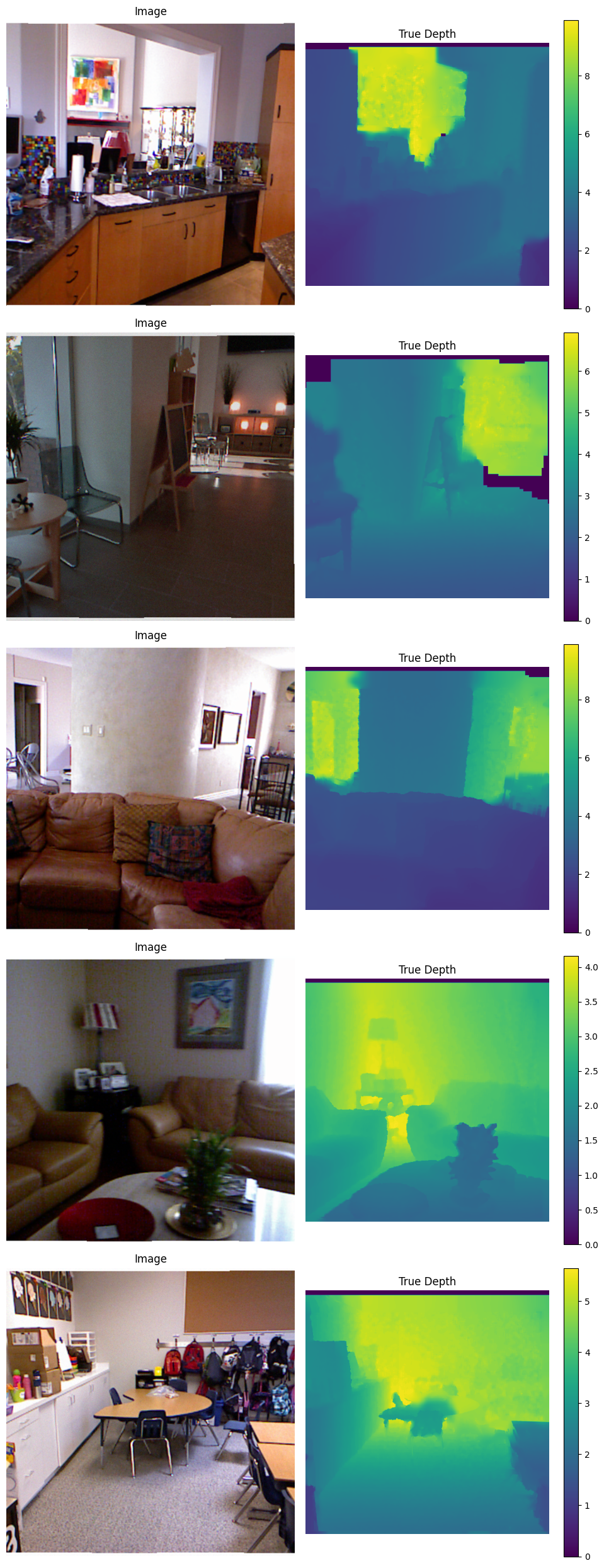
As you can see, the images are very blurry and noisy. Because of this, we won't be able to get fine-grained depth maps seen in the previews of Depth Anything V2. In the black hole artifacts, the depth is 0, and we will use this fact later for masking these holes. Also, the dataset contains many nearly identical photos of the same location.

Step 6: Prepare Dataloaders

def get_dataloaders(batch_size):
    
    train_dataset = NYU(train_paths, mode='train')
    val_dataset = NYU(val_paths, mode='val')
    
    
    train_dataloader = torch.utils.data.DataLoader(train_dataset, 
                                                  batch_size = batch_size,
                                                  shuffle=True,
                                                  num_workers=4,
                                                  drop_last=True
                                                  )

    val_dataloader = torch.utils.data.DataLoader(val_dataset, 
                                               batch_size = 1, #for dynamic resolution evaluations without padding
                                               shuffle=False,
                                               num_workers=4,
                                               drop_last=True
                                                )
    
    return train_dataloader, val_dataloader

Step 7: Metric Evaluation

def eval_depth(pred, target):
    assert pred.shape == target.shape

    thresh = torch.max((target / pred), (pred / target))

    d1 = torch.sum(thresh < 1.25).float() / len(thresh)

    diff = pred - target
    diff_log = torch.log(pred) - torch.log(target)

    abs_rel = torch.mean(torch.abs(diff) / target)

    rmse = torch.sqrt(torch.mean(torch.pow(diff, 2)))
    mae = torch.mean(torch.abs(diff))

    silog = torch.sqrt(torch.pow(diff_log, 2).mean() - 0.5 * torch.pow(diff_log.mean(), 2))

    return {'d1': d1.detach(), 'abs_rel': abs_rel.detach(),'rmse': rmse.detach(), 'mae': mae.detach(), 'silog':silog.detach()}

Our loss function is SiLog. It might seem that when training on absolute depth, we should forget about invariance to scale and other techniques used for relative depth training. However, it turns out this is not entirely true, and we often still want to use a kind of "scale regularization", but to a lesser extent. The parameter λ=0.5 helps balance between global consistency and local accuracy.

Step 8: Define Hyperparameters

model_weights_path =  '/kaggle/working/depth_anything_v2_vits.pth' 
model_configs = {
        'vits': {'encoder': 'vits', 'features': 64, 'out_channels': [48, 96, 192, 384]},
        'vitb': {'encoder': 'vitb', 'features': 128, 'out_channels': [96, 192, 384, 768]},
        'vitl': {'encoder': 'vitl', 'features': 256, 'out_channels': [256, 512, 1024, 1024]},
        'vitg': {'encoder': 'vitg', 'features': 384, 'out_channels': [1536, 1536, 1536, 1536]}
    }
model_encoder = 'vits'
max_depth = 10
batch_size = 11
lr = 5e-6
weight_decay = 0.01
num_epochs = 10
warmup_epochs = 0.5
scheduler_rate = 1
load_state = False

state_path = "/kaggle/working/cp"
save_model_path = '/kaggle/working/model'
seed = 42
mixed_precision = 'fp16'

Pay attention to the parameter "max_depth". The last layer in our model is a sigmoid for each pixel, producing an output from 0 to 1. We simply multiply each pixel by "max_depth" to represent distances from 0 to "max_depth".

Step 9: Training Function

def train_fn():

    set_seed(seed)
    ddp_kwargs = DistributedDataParallelKwargs(find_unused_parameters=True) 
    accelerator = Accelerator(mixed_precision=mixed_precision, 
                              kwargs_handlers=[ddp_kwargs],
                             )
    
    # in the paper they initialize decoder randomly and use only encoder pretrained weights. Then full fine-tune
    # ViT-S encoder here
    model = DepthAnythingV2(**{**model_configs[model_encoder], 'max_depth': max_depth})
    model.load_state_dict({k: v for k, v in torch.load(model_weights_path).items() if 'pretrained' in k}, strict=False)
    
    optim = torch.optim.AdamW([{'params': [param for name, param in model.named_parameters() if 'pretrained' in name], 'lr': lr},
                       {'params': [param for name, param in model.named_parameters() if 'pretrained' not in name], 'lr': lr*10}],
                      lr=lr, weight_decay=weight_decay)
    
    criterion = SiLogLoss() # author's loss
    
    train_dataloader, val_dataloader = get_dataloaders(batch_size)
    
    scheduler = transformers.get_cosine_schedule_with_warmup(optim, len(train_dataloader)*warmup_epochs, num_epochs*scheduler_rate*len(train_dataloader))
    
    model, optim, train_dataloader, val_dataloader, scheduler = accelerator.prepare(model, optim, train_dataloader, val_dataloader, scheduler)
    
    if load_state:
        accelerator.wait_for_everyone()
        accelerator.load_state(state_path)
        
    best_val_absrel = 1000
    
    
    for epoch in range(1, num_epochs):
        
        model.train()
        train_loss = 0
        for sample in tqdm(train_dataloader, disable = not accelerator.is_local_main_process):
            optim.zero_grad()
            
            img, depth = sample['image'], sample['depth']
            
            pred = model(img) 
                                                     # mask
            loss = criterion(pred, depth, (depth <= max_depth) & (depth >= 0.001))
            
            accelerator.backward(loss)
            optim.step()
            scheduler.step()
            
            train_loss += loss.detach()
            
            
        train_loss /= len(train_dataloader)
        train_loss = accelerator.reduce(train_loss, reduction='mean').item()
        
        
        model.eval()
        results = {'d1': 0, 'abs_rel': 0,'rmse': 0, 'mae': 0, 'silog': 0}
        for sample in tqdm(val_dataloader, disable = not accelerator.is_local_main_process):
            
            img, depth = sample['image'].float(), sample['depth'][0]
            
            with torch.no_grad():
                pred = model(img)
                # evaluate on the original resolution 
                pred = F.interpolate(pred[:, None], depth.shape[-2:], mode='bilinear', align_corners=True)[0, 0]
            
            valid_mask = (depth <= max_depth) & (depth >= 0.001)
            
            cur_results = eval_depth(pred[valid_mask], depth[valid_mask])
            
            for k in results.keys():
                results[k] += cur_results[k]
            

        for k in results.keys():
            results[k] = results[k] / len(val_dataloader)
            results[k] = round(accelerator.reduce(results[k], reduction='mean').item(),3)
        
        accelerator.wait_for_everyone()
        accelerator.save_state(state_path, safe_serialization=False)
        
        if results['abs_rel'] < best_val_absrel:
            best_val_absrel = results['abs_rel']
            unwrapped_model = accelerator.unwrap_model(model)
            if accelerator.is_local_main_process:
                torch.save(unwrapped_model.state_dict(), save_model_path)
        
        accelerator.print(f"epoch_{epoch},  train_loss = {train_loss:.5f}, val_metrics = {results}")
        
#P.S. While testing one configuration, I encountered an error in which the loss turned into nan. 
# This is fixed by adding a small epsilon to the predictions to prevent division by 0

In the paper, the authors randomly initialize the decoder and use only the encoder weights. They then fine-tune the entire model. Other notable points include:

• Using different learning rates for the decoder and encoder. The encoder’s learning rate is lower since we don't want to significantly alter the already excellent weights, unlike the randomly initialized decoder.
• The authors used a polynomial scheduler in the paper, while I used a cosine scheduler with warmup because I like it.
• In the mask, as mentioned earlier, we avoid the black holes in the depth maps by using the condition "depth >= 0.001"
• During training cycles, we calculate the loss on resized depth maps. During validation, we upsample the predictions and compute metrics at the original resolution.
• And look how easily we can wrap custom PyTorch code for distributed computing using HF accelerate.

Step 10: Launch the Training

#You can run this code with 1 gpu. Just set num_processes=1
notebook_launcher(train_fn, num_processes=2)

I believe we achieved our desired goal. The slight difference in performance can be attributed to the significant difference in dataset sizes (40k vs 400k). Keep in mind, we used the ViT-S encoder.

Let's show some results

model = DepthAnythingV2(**{**model_configs[model_encoder], 'max_depth': max_depth}).to('cuda')
model.load_state_dict(torch.load(save_model_path))

num_images = 10

fig, axes = plt.subplots(num_images, 3, figsize=(15, 5 * num_images))

val_dataset = NYU(val_paths, mode='val') 
model.eval()
for i in range(num_images):
    sample = val_dataset[i]
    img, depth = sample['image'], sample['depth']
    
    mean = torch.tensor([0.485, 0.456, 0.406]).view(3, 1, 1)
    std = torch.tensor([0.229, 0.224, 0.225]).view(3, 1, 1)
   
    with torch.inference_mode():
        pred = model(img.unsqueeze(0).to('cuda'))
        pred = F.interpolate(pred[:, None], depth.shape[-2:], mode='bilinear', align_corners=True)[0, 0]
            
    img = img*std + mean
     
    axes[i, 0].imshow(img.permute(1,2,0))
    axes[i, 0].set_title('Image')
    axes[i, 0].axis('off')

    max_depth = max(depth.max(), pred.cpu().max())
    
    im1 = axes[i, 1].imshow(depth, cmap='viridis', vmin=0, vmax=max_depth)
    axes[i, 1].set_title('True Depth')
    axes[i, 1].axis('off')
    fig.colorbar(im1, ax=axes[i, 1])
    
    im2 = axes[i, 2].imshow(pred.cpu(), cmap='viridis', vmin=0, vmax=max_depth)
    axes[i, 2].set_title('Predicted Depth')
    axes[i, 2].axis('off')
    fig.colorbar(im2, ax=axes[i, 2])

plt.tight_layout()

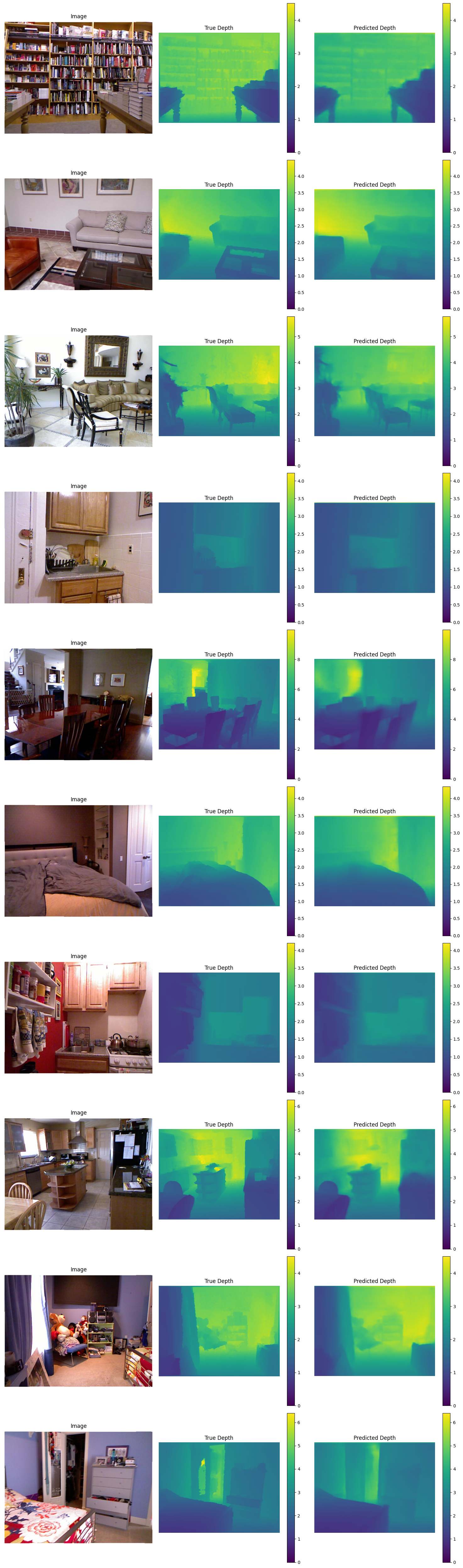
The images in the validation set are much cleaner and more accurate than those in the training set, which is why our predictions appear a bit blurry in comparison. Take another look at the training samples above.

In general, the key takeaway is that the model’s quality heavily depends on the quality of the provided depth maps. Kudos to the authors of Depth Anything V2 for overcoming this limitation and producing very sharp depth maps. The only drawback is that they are relative.

References

• Towards Robust Monocular Depth Estimation: Mixing Datasets for Zero-shot Cross-dataset Transfer
• ZoeDepth: Zero-shot Transfer by Combining Relative and Metric Depth
• Vision Transformers for Dense Prediction
• Depth Anything: Unleashing the Power of Large-Scale Unlabeled Data
• Depth Anything V2