Abstract
Reversible computing allows one to run programs not only in the usual forward direction, but also backward. A main application area for reversible computing is debugging, where one can use reversibility to go backward from a visible misbehaviour towards the bug causing it. While reversible debugging of sequential systems is well understood, reversible debugging of concurrent and distributed systems is less settled. We present here two approaches for debugging concurrent programs, one based on backtracking, which undoes actions in reverse order of execution, and one based on causal consistency, which allows one to undo any action provided that its consequences, if any, are undone beforehand. The first approach tackles an imperative language with shared memory, while the second one considers a core of the functional message-passing language Erlang. Both the approaches are based on solid formal foundations.
This work has been partially supported by COST Action IC1405 on Reversible Computation - Extending Horizons of Computing. The second author has been partially supported by the French National Research Agency (ANR), project DCore n. ANR-18-CE25-0007. The third author has been partially supported by JSPS KAKENHI Grant Number JP17H01722. The last author has been partially supported by the EU (FEDER) and the Spanish MICINN/AEI under grant TIN2016-76843-C4-1-R and by the Generalitat Valenciana under grant Prometeo/2019/098 (DeepTrust).
You have full access to this open access chapter, Download chapter PDF
1 Introduction
Reversible computing has been attracting interest due to its applications in fields as different as, e.g., hardware design [12], computational biology [4], quantum computing [2], discrete simulation [6] and robotics [31].
One of the oldest and more explored application areas for reversible computing is program debugging. This can be explained by looking, on the one hand, to the relevance of the problem, and, on the other hand, to how naturally reversible computing fits in the picture. Concerning the former, finding and fixing bugs inside software has always been a main activity in the software development life cycle. Indeed, according to a 2014 study [47], the cost of debugging amounts to $312 billions annually. Another recent study [3] estimates that the time spent in debugging is 49.9% of the total programming time. Concerning how naturally reversible computing fits in this context, consider that debugging means finding a bug, i.e., some wrong line of code, causing some visible misbehaviour, i.e., a wrong effect of a program, such as a wrong message printed on the screen. In general, the execution of the wrong line precedes the wrong visible effect. For instance, a wrong assignment to a variable may imply a misbehaviour later on, when the value of the variable is printed on the screen. Usually, the programmer has a very precise idea about which line of code makes the misbehaviour visible, but a non trivial debugging activity may be needed to find the bug. Indeed, debugging practice requires to put a breakpoint before the line of code where the programmer thinks the bug is, and use step-by-step execution from there to find the wrong line of code. However, the guess of the location of the bug is frequently wrong, causing the breakpoint to occur too late (after the bug) and a new execution with an updated guess is often needed. Reversible debugging practice is more direct: first, run the program and stop when the visible misbehaviour is reached; then, execute backwards (possibly step-by-step) looking for the causes of the misbehaviour until the bug is found.
With these premises, it is no surprise that reversible debugging has been deeply explored, as shown for instance by the survey in [11]. Indeed, many debuggers provide features for reversible execution, including popular open source debuggers such as GDB [8] as well as tools from big corporations such as Microsoft, the case of WinDbg [34].
However, the problem is far less settled for concurrent and distributed programs. We remark that nowadays most of the software is concurrent, either since the platform is distributed, the case of Internet or the Cloud, or to overcome the advent of the power wall [46]. Finding bugs in concurrent and distributed software is more difficult than in sequential software [33], since faults may appear or disappear according to the speed of the different processes and of the network communications. The bugs generating these faults, called Heisenbugs, are thus particularly challenging because they are rather difficult to reproduce. Two approaches to reversible debugging of concurrent systems have been proposed. Using backtracking,Footnote 1 actions are undone in reverse order of execution, while using causal-consistent reversibility [25] actions can be undone in any order, provided that the consequences of a given action, if any, are undone beforehand. Note that, by exploring a computation back and forth using either backtracking or causal-consistent reversibility one is guaranteed that Heisenbugs that occurred in the computation will not disappear.
This paper will present two lines of research on debugging for concurrent systems developed within the European COST Action IC1405 on “Reversible Computation - Extending Horizons of Computing” [23]. They share the use of state saving to enable backward computation (this is called a Landauer embedding [24], and it is needed to tackle languages which are irreversible) and a formal approach aiming at supporting debugging tools with a theory guaranteeing the desired properties. The first line of research [20,21,22] (Sect. 3) supports backtracking (apart from some non relevant actions) for a concurrent imperative language with shared memory, while the second line of research [28,29,30, 36] (Sect. 4) supports causal-consistent reversibility for a core subset of the functional message-passing language Erlang. We will showcase both the approaches on the same airline booking example (Sect. 2), coded in the two languages. Related work is discussed in Sect. 5 and final remarks are presented in Sect. 6.
2 Airline Booking Example
In this section we will introduce an example program that contains a bug, and discuss a specific execution leading to a corresponding misbehaviour. This example will be used as running example throughout the paper. We will show this example in the two programming languages needed for the two approaches mentioned above. We begin by introducing each of these languages.
2.1 Imperative Concurrent Language
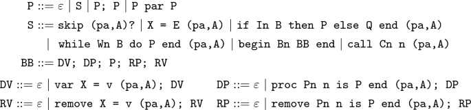
Our first language is much like any while language, consisting of assignments, conditional statements and while loops. Support has also been added for block statements containing the declaration of local variables and/or procedures, as well as procedure call statements. Further to this, removal statements are introduced to “clean up” at the end of a block, where any variables or procedures declared within the block are removed. Our language also contains unique names given to each conditional, loop, block, procedure declaration and call statement, named construct identifiers (represented as i1.0, w1.0, b1.0, etc.), and sequences of block names in which a given statement resides named paths (represented as pa). Both of these are used to handle variable scope, allowing one to distinguish different variables with the same name. The final addition to our language is interleaving parallel composition. A parallel statement, written P par Q allows the execution of the programs P and Q to interleave. All statements except blocks contain a stack A that is used to store identifiers (see below). The syntax of our language follows, where \(\varepsilon \) represents an empty program. Note that \(\varepsilon \) is the neutral element of sequential and parallel composition. We write (pa,A)? to denote the fact that (pa,A) is optional. We also write In, Wn, Bn, Cn to range, respectively, over identifiers for conditionals, while loops, blocks and call statements. Also, n refers to the name of a procedure.
Operational Semantics. Our approach (see [20] for a detailed explanation) to reversing programs starts by producing two versions of the original program. The first one, named the annotated version, performs forward execution and saves any information that would be lost in a normal computation but is needed for inversion (named reversal information and saved into our auxiliary store \(\delta \)). Identifiers are assigned to statements as we execute them, capturing the interleaving order needed for correct inversion. The second one, named the inverted version, executes forwards but simulates reversal using the reversal information as well as the identifiers to follow backtracking order. We comment here that we use ‘inversion’ to refer to both the process of producing the program code of the inverted version (program inverter [1]), and to the process of executing the inverted version of a program. A reverse execution computes all parallel statements as in a forward execution, but it uses identifiers to determine which statement to invert next (instead of nondeterministically deciding). For programs containing many nested parallel statements, the overhead of determining the correct interleaving order increases, though we still deem this as reasonable [19]. Note that using a nondeterministic interleaving for the reverse execution is not possible, since it is not guaranteed to behave correctly (e.g., requiring information from the auxiliary store that is not there may cause an execution to be stuck). However, a small number of execution steps, including closing a block and removing a skip, do not use an identifier and can therefore be interleaved nondeterministically during an inverse execution. Forward and reverse execution are each defined in terms of a non-standard, small step operational semantics. Our semantics perform both the expected execution (forward and reverse respectively) and all necessary saving/using of the reversal information. Consider the example rule [D1a] for assignments, which is a reversibilisation of the traditional irreversible semantics of an assignment statement [51].

As shown here, this rule consists of the evaluation of the expression e to the value v, evaluation of the variable X to a memory location l and finally the assigning of the value v to the memory location l as expected. Alongside this, the rule also pushes the old value of the variable (the current value held at the memory location, namely \(\sigma (\texttt {l})\)) onto the stack for this variable name within \(\delta \) (
 , where
 denotes a push operation). This old value is saved alongside the next available identifier m, returned via the function next() and used within the rule to record interleaving order (represented using the labelled arrow \(\xrightarrow {m}\)). This identifier m is also inserted into the stack A corresponding to this specific assignment statement, represented as m:A.
Now consider the rule [D1r] from our inverse semantics for reversing assignments (that executed forwards via [D1a]).

This rule first ensures this is the next statement to invert using the identifier m, which must match the last used identifier (previous()) and be present in both the statements stack (A = m:A\('\)) and the auxiliary store alongside the old value (\(\delta (\texttt {X}) = \texttt {(m,v):X}'\)). Provided this is satisfied, this rule then removes all occurrences of m, and assigns the old value v retrieved from \(\delta \) to the corresponding memory location. Note that e appears exactly as in the original version but it is not evaluated, and that the functions next() and previous() both update the next and previous identifiers respectively as a side effect.
2.2 Erlang
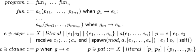
Our second approach deals with a relevant fragment of the functional and concurrent language Erlang. We show in Fig. 1 the syntax of its main constructs, focusing on the ones needed in our running example. We drop from the syntax some declarations related to module management, which are orthogonal to our purpose in this paper.
Language syntax rules
A program is a sequence of function definitions, where each function has a name (an atom, denoted by a) and is defined by a number of equations of the form \(a_i(p_{i1},~\ldots ,~p_{in_i})~\mathsf {when}~g_i \rightarrow e_i\), where \(p_{i1},~\ldots ,~p_{in_i}\) are patterns (i.e., terms built from variables and data constructors), \(g_i\) is a guard (typically an arithmetic or relational expression only involving built-in functions), and \(e_i\) is an arbitrary expression. As is common, the variables in \(p_{i1},~\ldots ,~p_{in_i}\) are the only variables that may occur free in \(g_i\) and \(e_i\). The body of a function is an expression, which can include variables, literals (i.e., atoms, integers, floating point numbers, the empty list \([\,]\), etc.), lists (using Prolog-like notation, i.e., \([e_1|e_2]\) is a list with head \(e_1\) and tail \(e_2\)), tuples (denoted by \(\{e_1,\ldots ,e_n\}\)),Footnote 2 function applications (we do not consider higher order functions in this paper for simplicity), pattern matching, sequences (denoted by comma), receive expressions, \(\mathsf {spawn}\) (for creating new processes), “!” (for sending a message), and \(\mathsf {self}\). Note that some of these functions are actually built-ins in Erlang.
In contrast to expressions, patterns are built from variables, literals, lists, and tuples. Patterns can only contain fresh variables. In turn, values are built from literals, lists, and tuples (i.e., values are ground patterns). In Erlang, variables start with an uppercase letter.
Let us now informally introduce the semantics of Erlang constructions. In the following, substitutions are denoted by Greek letters \(\sigma \), \(\theta \), etc. A substitution \(\sigma \) denotes a mapping from variables to expressions, where \({\mathcal {D}om}(\sigma )\) is its domain. Substitution application \(\sigma (e)\) is also denoted by \(e\sigma \).
Given the pattern matching \( p =e\), we first evaluate e to a value, say v; then, we check whether v matches p, i.e., there exists a substitution \(\sigma \) for the variables of p with \(v=p\sigma \) (otherwise, an exception is raised). Then, the expression reduces to v, and variables are bound according to \(\sigma \). Roughly speaking, a sequence \((p=e_1,\, e_2)\) is equivalent to the expression \(\mathsf {let}~p=e_1~\mathsf {in}~e_2\) in most functional programming languages.
A similar pattern matching operation is performed during a function application \(a(e_1,\ldots ,e_n)\). First, one evaluates \(e_1,\ldots ,e_n\) to values, say \(v_1,\ldots ,v_n\). Then, we scan the left-hand sides of the equations defining the function a until we find one that matches \(a(v_1,\ldots ,v_n)\). Let \(a(p_1,\ldots ,p_n)~\mathsf {when}~g\rightarrow e\) be such equation, with \(a(v_1,\ldots ,v_n)=a(p_1,\ldots ,p_n)\sigma \). Here, we should also check that the guard, \(g\sigma \), reduces to true. In this case, execution proceeds with the evaluation of the function’s body, \(e\sigma \).
Let us now consider the concurrent features of our language. In Erlang, a running system can be seen as a pool of processes that can only interact through message sending and receiving (i.e., there is no shared memory). Received messages are stored in the queues of processes until they are consumed; namely, each process has one associated local (FIFO) queue. A process is uniquely identified by its pid (process identifier). Message sending is asynchronous, while receive instructions block the execution of a process until an appropriate message reaches its local queue (see below).
We consider the following functions with side-effects: \(\mathsf {self}\), “!”, \(\mathsf {spawn}\), and \(\mathsf {receive}\). The expression \(\mathsf {self}()\) returns the pid of a process, while \(\mathrm {p}\,!\,v\) evaluates to v and, as a side-effect, sends message v to the process with pid \(\mathrm {p}\), which will be eventually stored in \(\mathrm {p}\)’s local queue. New processes are spawned with a call of the form \(\mathsf {spawn}(mod,a,[v_1,\ldots ,v_n])\), where mod is the name of the module declaring function a, and the new process begins with the evaluation of the function application \(a(v_1,\ldots ,v_n)\). The expression \(\mathsf {spawn}(mod,a,[v_1,\ldots ,v_n])\) returns the (fresh) pid assigned to the new process.
Finally, an expression “\(\mathsf {receive}~p_1 ~\mathsf {when} ~g_1\rightarrow e_1;\ldots ; p_n ~\mathsf {when} ~g_n\rightarrow e_n~\mathsf {end}\)” should find the first message v in the process’ queue (if any) such that v matches some pattern \(p_i\) (with substitution \(\sigma \)) and the instantiation of the corresponding guard \(g_i\sigma \) reduces to true. Then, the receive expression evaluates to \(e_i\sigma \), with the side effect of deleting the message v from the process’ queue. If there is no matching message in the current queue, the process suspends until a matching message arrives.
2.3 Airline Code
We are now ready to describe the example. Consider a model of an airline booking system, where multiple agents sell tickets for the same flight. In order to keep the example concise, we consider only two agents selling tickets in parallel, with three seats initially available. The code of the example is shown in Listing 1.1, written in the concurrent imperative programming language described in Sect. 2.1.
The code contains two while loops operating in parallel (lines 10–16 and 18–24), where each loop models the operation of a single agent. Let us consider the first loop. For each iteration, the agent checks whether any seat remains (line 11). As long as the number of currently available seats is greater than zero, the agent is free to sell a ticket via the procedure named sell (called at line 12). Once the number of available tickets has reached zero, each agent will then close, terminating its loop.
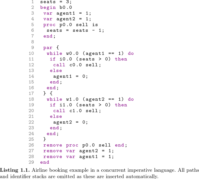
As previously mentioned, this program can show a misbehaviour under certain execution paths. Recall the simplified setting of three initially available seats. Consider an execution that begins with each agent selling a single ticket (allocating one seat) via one full iteration of each while loop (the interleaving among the two iterations is not relevant). At this point, both agents remain open (since agent1 = 1 and agent2 = 1), and the current number of seats is 1. Now assume that the execution continues with the following interleaving. The condition of each while loop is checked, both of which will evaluate to true as each agent is open. Next, the execution of each loop body begins with the evaluation of the guard of each conditional statement. They will both evaluate to true, as there is at least one seat available. At this point, each agent is committed to selling one more ticket, even if only one seat is available. The rest of the execution can then be finished under any interleaving. The important thing to note here is that the final number of free seats is -1. This is an obvious misbehaviour, as the two agents allocated four tickets when only three seats were available. This misbehaviour occurs since the programmer assumed that the checking for an available seat and its allocation were atomic, but there is no mechanism enforcing this.
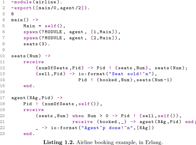
Listing 1.2 shows the same example coded in Erlang. A call to the initial function, main, spawns two processes (the agents) that start with the execution of function calls agent(1,Main) and agent(2,Main), respectively. Here, Main is a variable with the pid of the main process, which is obtained via a call to the predefined function self.
Then, at line 8, the main process calls to function seats with argument 3 (the initial number of available seats). From this point on, the main process behaves as a server that executes a potentially infinite loop that waits for requests and replies to them. Here, the state of the process is given by the argument Num which represents the current number of available seats. The server accepts two kinds of messages: {numOfSeats,Pid}, a request to know the current number of available seats, and {sell,Pid}, to decrease the number of available seats (analogously to the procedure sell in Listing 1.1). In the first case, the number of available seats is sent back to the agent that performed the request (Pid ! Num); in the second case, the number of the booked seat is sent.Footnote 3 The behaviour of the agents (lines 17–23) is simple. An agent first sends a request to know the number of available seats, Pid ! {numOfSeats,self()}, where self() is required for the main process to be able to send a reply back to the sender. Then, the agent suspends its execution waiting for an answer {seats,Num}: if Num is greater than zero, the agent sends a new message to sell a seat (Pid ! {sell,self()}) and receives the confirmation ({booked,_});Footnote 4 otherwise, it terminates the execution with the message “AgentN done!”, where N is either 1 or 2.
3 Backtracking in a Concurrent Imperative Language
In this section we describe a state-saving approach to reversibility in the concurrent imperative programming language described in Sect. 2.1. We begin by discussing our approach and its use within the debugging of the airline example (see Sect. 2.3), along with our simulation tool [20, 21].

Final annotated and inverted versions of the airline example, with paths omitted
As described in more detail in [21], we have produced a simulator implementing the operational semantics of our approach. This simulator is capable of parsing a program, automatically inserting removal statements, construct identifiers and paths, and simulating both forward and reverse execution. Each execution can be either end-to-end, or step-by-step.

Stopping position of the inverse execution (containing paths automatically inserted by the simulator)
We first execute the forward version of our airline example completely. This execution produces the annotated version in Fig. 2a, where the identifier stack for each statement has been populated capturing an interleaving order that experiences the bug as outlined in Sect. 2.3. The inverted version of the airline example is shown in Fig. 2b, where the overall statement order has been inverted. Note that some annotations are omitted to keep this source code concise (e.g., no paths are shown). We start the debugging process at the beginning of the execution of the inverted version (line 1 of Fig. 2b). Recall that all expressions or conditions are not evaluated or used during an inverse execution. Using the final program state showing the misbehaviour (produced via the annotated execution with seats = -1), the simulator begins by opening the block and re-declaring both local variables and the procedure, using identifiers 40–38. From here, the execution continues with the parallel statement. The final iteration of each while loop is reversed (simulating the inversion of the closing of each agent) using identifiers 37–28. Now the penultimate iteration of each while loop must be inverted. The consecutive identifiers 27 and 26 are then used to ensure that each of the conditional statements (lines 11 and 19) are opened, using two true values retrieved from the reversal information saved.
The execution then continues using identifiers 25–20, where each loop almost completes the current iteration, reversing the last time each of them allocated a seat. This produces the state where seats = 1, and where the next available step is to close either of the inverse conditional statements. Though the identifiers ensure we must start by closing the conditional with identifier 19, the fact that both can be closed implies that both are open at the same time. This current position within the inverse execution is shown in Fig. 3, where the command ‘display loops’ outputs all current while loops (agents) with arrows indicating the next statement to be executed. It is clear from our semantics (see [20]) that the closing of an inverted conditional is the reverse of opening its forward version. Since the two conditionals have been opened using consecutive identifiers, one can see that each committed to selling a ticket. Given that the current state has seats = 1, this execution commits to selling two tickets when only one remains. It is therefore clear that this is an atomicity violation, since interleaving of other actions is allowed between the checking for at least one free seat and the allocation of it. We have therefore shown how the simulator implementing our approach to reversibility can be used during the debugging process of an example bug.
4 Causal-Consistent Reversibility in Erlang
In this section we will discuss how to apply causal-consistent reversible debugging to the airline booking example in Sect. 2.3. Our approach to reversible debugging is based on the following principles [29, 30]:
-
First, we consider a reduction semantics for the language (a subset of Core Erlang [5], which is an intermediate step in Erlang compilation). Our semantics includes two transition relations, one for expressions (which is mostly a call-by-value semantics for a functional language) and one for systems, i.e., collections of processes, possibly interacting through message passing. An advantage of this modular design is that only the transition relation for systems needs to be modified in order to produce a reversible semantics.
-
Then, we instrument the standard semantics in different ways. On the one hand, we instrument it to produce a log of the computation; namely, by recording all actions involving the sending and receiving of messages, as well as the spawning of new processes (see [30] for more details). On the other hand, one can instrument the semantics so that the configurations now carry enough information to undo any execution step, i.e., a typical Landauer embedding. Producing then a backward semantics that proceeds in the opposite direction is not difficult. Here, the configurations may include both a log—to drive forward executions—and a history—to drive backward executions.
-
It is worthwhile to note that forward computations need not follow exactly the same steps as in the recorded computation (indeed the log does not record the total order of steps). However, it is guaranteed that the admissible computations are causally equivalent to the recorded one; namely, they differ only for swaps of concurrent actions. Analogously, backward computations need not be the exact inverse of the considered forward computation, but ensuring that backward steps are causal-consistent suffices. This degree of freedom is essential to allow the user to focus on the process and/or actions of interest during debugging, rather than inspecting the complete execution (which is often impractical).
-
Finally, we define another layer on top of the reversible semantics in order to drive it following a number of requests from the user, e.g., rolling back up to the point where a given process was spawned, going forward up to the point where a message is sent, etc. This layer essentially implements a stack of requests that follows the causal dependencies of the reversible semantics.
In the following, we consider the causal-consistent reversible debugger CauDEr [27, 28] which follows the principles listed above.
CauDEr first translates the airline example into Core Erlang [5]. Then one can execute the program, either using a built-in scheduler, or using the log of an actual execution [30].
Here, if we compile the program in the standard environment and execute the call main(), we get the following output:
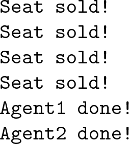
which is clearly incorrect since we only had three seats available.
By using the logger and, then, loading both the program and the log into CauDEr (as described in [30]), we can replay the entire execution and explore the sequence of concurrent actions. Figure 4 shows the final state (on the left) and the sequence of concurrent actions (on the right), where process 63 is the main process, and processes 67 and 68 are the agents.

CauDEr debugging session
Now, we can look at the sequence of concurrent actions, where messages are labelled with a unique identifier, added by CauDEr, which is shown in brackets to the right of the corresponding line:
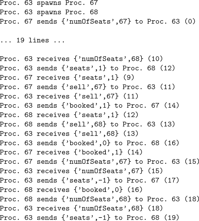
One can see that seat number 0 (which does not exist!) has been booked by process 68, and the notification has been provided via message number 16.
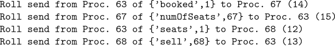
A good state to explore is the one where message number 16 has been sent. Here a main feature of causal-consistent reversible debugging comes handy: the possibility of going to the state just before a relevant action has been performed, by undoing it, including all and only its consequences. This is called a causal-consistent rollback. CauDEr provides causal-consistent rollbacks for various actions, including send actions. Thus, the programmer can invoke a Roll send command with message identifier 16 as a parameter.
In this way, one discovers that the message has been sent by process 63 (as expected, since process 63 is the main process). By exploring its state one understands that, from the point of view of process 63, sending message 16 is correct, since it is the only possible answer to a sell message. The bug should be thus before.
From the program code, the programmer knows that whether seat Num is available or not is checked by a message of the form {numOfSeats,Pid}, which is answered with a message of the form {seats,Num}, where Num is the number of available seats.
Looking again at the concurrency actions, the programmer can see that process number 68 was indeed notified of the availability of a seat by message number 12.
We can use again Roll send, now with parameter 12, to check whether this send is correct or not. We discover that indeed the send is correct since, when the message is sent, there is one available seat. However, here, another window comes handy: the Roll log window that shows which actions (causally dependent on the one undone) have been undone during a rollback, which shows:
By checking it the programmer sees that also the interactions between process 67 and process 63 booking seat 1 are undone. Hence the problem is that, in between the check for availability and the booking, another process may interact with main, stealing the seat; thus, the error is an atomicity violation.
Of course, given the simplicity of the system, one could have spotted the bug directly by looking at the code or at the full sequence of message exchanges, but the technique above is quite driven by the visible misbehaviour, hence it will better scale to larger systems (e.g., with more seats and agents, or with additional functionalities).
We remark that, while the presentation above concentrates on the debugger and its practical use, this line of research also deeply considered its theoretical underpinning, as briefly summarised at the beginning of the section. Thanks to this, relevant properties have been proved, e.g., that if a misbehaviour occurs in a computation then the same misbehaviour will occur also in each replay [30].
5 Related Work
Reversible computation in general, and reversible debugging in particular, have been deeply explored in the literature.
A line of research considers naturally reversible languages, that is languages where only reversible programs can be written. Such approaches include the imperative languages Janus [49, 50], R-CORE [17] and R-WHILE [16], and the object-oriented languages Joule [43] and ROOPL [18]. These approaches require dedicated languages, and cannot be applied to mainstream languages like Erlang or a classic imperative language, as we do in this paper.
The backtracking approach has been applied, e.g., in the Reverse C Compiler (RCC) defined by Perumalla et al. [6, 37]. It supports the entire programming language C, but lacks a proof of correctness, which is instead provided by our approaches. The Backstroke framework [48] is a further example, supporting the vast majority of the programming language C++. This framework has been used to provide reverse execution in the field of Parallel Discrete Event Simulation (PDES) [13], as described in more recent works by Schordan et al. [40,41,42]. Similar approaches have been used for debugging, e.g., based on program instrumentation techniques [7]. Identifiers and keys are used to control execution in the work by Phillips and Ulidowski [38, 39]. Another related work is omniscient debugging, where each assignment and method call is stored in an execution history, which can be used to restore any desired program state. An example of such a debugger written for Java was proposed by Lewis [32].
Causal-consistent reversibility has been mainly studied in the area of foundational process calculi such as CCS [10] and its variants [35, 38], \(\pi \)-calculus [9], and higher-order \(\pi \)-calculus [26] and coordination languages such as Klaim [15]. The application to debugging has been first proposed in [14] in the context of the toy functional language \(\mu \)Oz. A related approach is Actoverse [44], for Akka-based applications. It provides many relevant features complementary to ours, such as a partial-order graphical representation of message exchanges. On the other side, Actoverse allows one to explore only some states of the computation, such as the ones corresponding to message sending and receiving. We also mention Causeway [45], which however is not a full-fledged debugger, but just a post-mortem traces analyser.
6 Conclusion
We presented two approaches to reversible debugging of concurrent systems, we will now briefly compare them. Beyond the language they consider, the main difference between the two approaches is in the order in which execution steps can be reversed. The backtracking approach undoes them in reverse order of execution. This means that there is no need to track dependencies, and the user of the debugger can easily anticipate which steps will be undone by looking at identifiers. The causal-consistent approach instead allows independent steps of an execution to be reversed in any order, hence tracking dependencies between steps is crucial. This offers the benefit that only the steps strictly needed to reach the desired point of an execution need to be reversed, and steps which happened in between but were actually independent are disregarded.
Debugging is a relevant application area for reversible computation, but reversible debugging for concurrent and distributed systems is still in its infancy. While different techniques have been put forward, they are not yet able to deal with real, complex systems. A first reason is that they do not tackle mainstream languages (Erlang could be considered mainstream, but only part of the language is currently covered). When this first step will be completed, then runtime overhead and size of the logs will become relevant problems, as they are now in the setting of sequential reversible debugging.
Notes
- 1.
Backtracking sometimes refer to the exploration of a set of possibilities: this is not the case here, since backward execution is (almost) deterministic.
- 2.
The only data constructors in Erlang (besides literals) are the predefined functions for lists and tuples.
- 3.
We note that the number of the booked seat, \(\mathtt Num\), is not used by function \(\mathtt agent\) in our example, but might be used in a more realistic program. We keep this value anyway since it will ease the understanding of the trace in Sect. 4.
- 4.
Anonymous variables are denoted by an underscore “\(\_\)”.
References
Abramov, S., Glück, R.: Principles of inverse computation and the universal resolving algorithm. In: Mogensen, T.Æ., Schmidt, D.A., Sudborough, I.H. (eds.) The Essence of Computation. LNCS, vol. 2566, pp. 269–295. Springer, Heidelberg (2002). https://doi.org/10.1007/3-540-36377-7_13
Altenkirch, T., Grattage, J.: A functional quantum programming language. In: Proceedings of the 20th IEEE Symposium on Logic in Computer Science (LICS 2005), pp. 249–258. IEEE Computer Society (2005). https://doi.org/10.1109/LICS.2005.1
Britton, T., Jeng, L., Carver, G., Cheak, P., Katzenellenbogen, T.: Reversible debugging software - quantify the time and cost saved using reversible debuggers (2012). http://www.roguewave.com
Cardelli, L., Laneve, C.: Reversible structures. In: Fages, F. (ed.) Proceedings of the 9th International Conference on Computational Methods in Systems Biology (CMSB 2011), pp. 131–140. ACM (2011). https://doi.org/10.1145/2037509.2037529
Carlsson, R., et al.: Core Erlang 1.0.3. language specification (2004). https://www.it.uu.se/research/group/hipe/cerl/doc/core_erlang-1.0.3.pdf
Carothers, C.D., Perumalla, K.S., Fujimoto, R.: Efficient optimistic parallel simulations using reverse computation. ACM Trans. Model. Comput. Simul. 9(3), 224–253 (1999)
Chen, S., Fuchs, W.K., Chung, J.: Reversible debugging using program instrumentation. IEEE Trans. Softw. Eng. 27(8), 715–727 (2001). https://doi.org/10.1109/32.940726
Conrod, J.: Tutorial: reverse debugging with GDB 7 (2009). http://jayconrod.com/posts/28/tutorial-reverse-debugging-with-gdb-7
Cristescu, I., Krivine, J., Varacca, D.: A compositional semantics for the reversible \(\pi \)-calculus. In: Proceedings of the 28th Annual ACM/IEEE Symposium on Logic in Computer Science (LICS 2013), pp. 388–397. IEEE Computer Society (2013). https://doi.org/10.1109/LICS.2013.45
Danos, V., Krivine, J.: Reversible communicating systems. In: Gardner, P., Yoshida, N. (eds.) CONCUR 2004. LNCS, vol. 3170, pp. 292–307. Springer, Heidelberg (2004). https://doi.org/10.1007/978-3-540-28644-8_19
Engblom, J.: A review of reverse debugging. In: Morawiec, A., Hinderscheit, J. (eds.) Proceedings of the 2012 System, Software, SoC and Silicon Debug Conference (S4D), pp. 28–33. IEEE (2012)
Frank, M.P.: Introduction to reversible computing: motivation, progress, and challenges. In: Bagherzadeh, N., Valero, M., Ramírez, A. (eds.) Proceedings of the Second Conference on Computing Frontiers, pp. 385–390. ACM (2005). https://doi.org/10.1145/1062261.1062324
Fujimoto, R.: Parallel discrete event simulation. Commun. ACM 33(10), 30–53 (1990). https://doi.org/10.1145/84537.84545
Giachino, E., Lanese, I., Mezzina, C.A.: Causal-consistent reversible debugging. In: Gnesi, S., Rensink, A. (eds.) FASE 2014. LNCS, vol. 8411, pp. 370–384. Springer, Heidelberg (2014). https://doi.org/10.1007/978-3-642-54804-8_26
Giachino, E., Lanese, I., Mezzina, C.A., Tiezzi, F.: Causal-consistent rollback in a tuple-based language. J. Log. Algebraic Meth. Program. 88, 99–120 (2017)
Glück, R., Yokoyama, T.: A linear-time self-interpreter of a reversible imperative language. Comput. Softw. 33(3), 108–128 (2016)
Glück, R., Yokoyama, T.: A minimalist’s reversible while language. IEICE Trans. 100-D(5), 1026–1034 (2017)
Haulund, T.: Design and implementation of a reversible object-oriented programming language. Master’s thesis, Faculty of Science, University of Copenhagen (2017). https://arxiv.org/abs/1707.07845
Hoey, J.: Reversing an imperative concurrent programming language. Ph.D. thesis, University of Leicester (2020)
Hoey, J., Ulidowski, I., Yuen, S.: Reversing imperative parallel programs with blocks and procedures. In: 2018 Proceedings of Express/SOS (2018)
Hoey, J., Ulidowski, I.: Reversible imperative parallel programs and debugging. In: Thomsen, M.K., Soeken, M. (eds.) RC 2019. LNCS, vol. 11497, pp. 108–127. Springer, Cham (2019). https://doi.org/10.1007/978-3-030-21500-2_7
Hoey, J., Ulidowski, I., Yuen, S.: Reversing parallel programs with blocks and procedures. In: Pérez, J.A., Tini, S. (eds.) Proceedings of the Combined 25th International Workshop on Expressiveness in Concurrency and 15th Workshop on Structural Operational Semantics (EXPRESS/SOS 2018), EPTCS, vol. 276, pp. 69–86 (2018). https://doi.org/10.4204/EPTCS.276.7
European COST actions IC1405 on “reversible computation - extending horizons of computing”. http://www.revcomp.eu/
Landauer, R.: Irreversibility and heat generated in the computing process. IBM J. Res. Dev. 5, 183–191 (1961)
Lanese, I., Mezzina, C.A., Tiezzi, F.: Causal-consistent reversibility. Bull. EATCS 114, 121–139 (2014)
Lanese, I., Mezzina, C.A., Stefani, J.B.: Reversibility in the higher-order \(\pi \)-calculus. Theor. Comput. Sci. 625, 25–84 (2016)
Lanese, I., Nishida, N., Palacios, A., Vidal, G.: CauDEr. https://github.com/mistupv/cauder
Lanese, I., Nishida, N., Palacios, A., Vidal, G.: CauDEr: a causal-consistent reversible debugger for Erlang. In: Gallagher, J.P., Sulzmann, M. (eds.) FLOPS 2018. LNCS, vol. 10818, pp. 247–263. Springer, Cham (2018). https://doi.org/10.1007/978-3-319-90686-7_16
Lanese, I., Nishida, N., Palacios, A., Vidal, G.: A theory of reversibility for Erlang. J. Log. Algebraic Meth. Program. 100, 71–97 (2018)
Lanese, I., Palacios, A., Vidal, G.: Causal-consistent replay debugging for message passing programs. In: Pérez, J.A., Yoshida, N. (eds.) FORTE 2019. LNCS, vol. 11535, pp. 167–184. Springer, Cham (2019). https://doi.org/10.1007/978-3-030-21759-4_10
Laursen, J.S., Schultz, U.P., Ellekilde, L.: Automatic error recovery in robot assembly operations using reverse execution. In: Proceedings of the 2015 IEEE/RSJ International Conference on Intelligent Robots and Systems (IROS 2015), pp. 1785–1792. IEEE (2015). https://doi.org/10.1109/IROS.2015.7353609
Lewis, B.: Debugging backwards in time. In: Ronsse, M., Bosschere, K.D. (eds.) Proceedings of the Fifth International Workshop on Automated Debugging (AADEBUG 2003), pp. 225–235 (2003). https://arxiv.org/abs/cs/0310016
Lu, S., Park, S., Seo, E., Zhou, Y.: Learning from mistakes: a comprehensive study on real world concurrency bug characteristics. In: Eggers, S.J., Larus, J.R. (eds.) Proceedings of the 13th International Conference on Architectural Support for Programming Languages and Operating Systems (ASPLOS 2008), pp. 329–339. ACM (2008). https://doi.org/10.1145/1346281.1346323
McNellis, J., Mola, J., Sykes, K.: Time travel debugging: root causing bugs in commercial scale software. CppCon talk (2017). https://www.youtube.com/watch?v=l1YJTg_A914
Mezzina, C.A.: On reversibility and broadcast. In: Kari, J., Ulidowski, I. (eds.) RC 2018. LNCS, vol. 11106, pp. 67–83. Springer, Cham (2018). https://doi.org/10.1007/978-3-319-99498-7_5
Nishida, N., Palacios, A., Vidal, G.: A reversible semantics for Erlang. In: Hermenegildo, M.V., Lopez-Garcia, P. (eds.) LOPSTR 2016. LNCS, vol. 10184, pp. 259–274. Springer, Cham (2017). https://doi.org/10.1007/978-3-319-63139-4_15
Perumalla, K.: Introduction to Reversible Computing. CRC Press, Boca Raton (2014)
Phillips, I., Ulidowski, I.: Reversing algebraic process calculi. J. Log. Algebraic Program. 73(1–2), 70–96 (2007)
Phillips, I., Ulidowski, I., Yuen, S.: A reversible process calculus and the modelling of the ERK signalling pathway. In: Glück, R., Yokoyama, T. (eds.) RC 2012. LNCS, vol. 7581, pp. 218–232. Springer, Heidelberg (2013). https://doi.org/10.1007/978-3-642-36315-3_18
Schordan, M., Jefferson, D., Barnes, P., Oppelstrup, T., Quinlan, D.: Reverse code generation for parallel discrete event simulation. In: Krivine, J., Stefani, J.-B. (eds.) RC 2015. LNCS, vol. 9138, pp. 95–110. Springer, Cham (2015). https://doi.org/10.1007/978-3-319-20860-2_6
Schordan, M., Oppelstrup, T., Jefferson, D.R., Barnes Jr., P.D.: Generation of reversible C++ code for optimistic parallel discrete event simulation. New Gener. Comput. 36(3), 257–280 (2018). https://doi.org/10.1007/s00354-018-0038-2
Schordan, M., Oppelstrup, T., Jefferson, D.R., Barnes Jr, P.D., Quinlan, D.J.: Automatic generation of reversible C++ code and its performance in a scalable kinetic Monte-Carlo application. In: Fujimoto, R., Unger, B.W., Carothers, C.D. (eds.) Proceedings of the 2016 Annual ACM Conference on SIGSIM Principles of Advanced Discrete Simulation (SIGSIM-PADS 2016), pp. 111–122. ACM (2016). https://doi.org/10.1145/2901378.2901394
Schultz, U.P., Axelsen, H.B.: Elements of a reversible object-oriented language. In: Devitt, S., Lanese, I. (eds.) RC 2016. LNCS, vol. 9720, pp. 153–159. Springer, Cham (2016). https://doi.org/10.1007/978-3-319-40578-0_10
Shibanai, K., Watanabe, T.: Actoverse: a reversible debugger for actors. In: Proceedings of the 7th ACM SIGPLAN International Workshop on Programming Based on Actors, Agents, and Decentralized Control (AGERE 2017), pp. 50–57. ACM (2017). https://doi.org/10.1145/3141834.3141840
Stanley, T., Close, T., Miller, M.S.: Causeway: a message-oriented distributed debugger. Technical report, HP Labs tech report HPL-2009-78 (2009). http://www.hpl.hp.com/techreports/2009/HPL-2009-78.html
Sutter, H.: The free lunch is over: a fundamental turn toward concurrency in software. Dr. Dobb’s J. 30(3), 202–210 (2005)
Undo Software: Increasing software development productivity with reversible debugging (2014). http://undo-software.com/wp-content/uploads/2014/10/Increasing-software-development-productivity-with-reversible-debugging.pdf
Vulov, G., Hou, C., Vuduc, R.W., Fujimoto, R., Quinlan, D.J., Jefferson, D.R.: The backstroke framework for source level reverse computation applied to parallel discrete event simulation. In: Jain, S., Creasey Jr, R.R.., Himmelspach, J., White, K.P., Fu, M.C. (eds.) Proceedings of the Winter Simulation Conference (WSC 2011), pp. 2965–2979. IEEE (2011). https://doi.org/10.1109/WSC.2011.6147998
Yokoyama, T., Glück, R.: A reversible programming language and its invertible self-interpreter. In: Ramalingam, G., Visser, E. (eds.) Proceedings of the 2007 ACM SIGPLAN Workshop on Partial Evaluation and Semantics-Based Program Manipulation (PEPM 2007), pp. 144–153. ACM (2007)
Yokoyama, T., Axelsen, H.B., Glück, R.: Principles of a reversible programming language. In: Ramírez, A., Bilardi, G., Gschwind, M. (eds.) Proceedings of the 5th Conference on Computing Frontiers, pp. 43–54. ACM (2008). https://doi.org/10.1145/1366230.1366239
Yokoyama, T., Axelsen, H.B., Glück, R.: Fundamentals of reversible flowchart languages. Theor. Comput. Sci. 611, 87–115 (2016). https://doi.org/10.1016/j.tcs.2015.07.046
Author information
Authors and Affiliations
Corresponding author
Editor information
Editors and Affiliations
Rights and permissions
Open Access This chapter is licensed under the terms of the Creative Commons Attribution 4.0 International License (http://creativecommons.org/licenses/by/4.0/), which permits use, sharing, adaptation, distribution and reproduction in any medium or format, as long as you give appropriate credit to the original author(s) and the source, provide a link to the Creative Commons license and indicate if changes were made.
The images or other third party material in this chapter are included in the chapter's Creative Commons license, unless indicated otherwise in a credit line to the material. If material is not included in the chapter's Creative Commons license and your intended use is not permitted by statutory regulation or exceeds the permitted use, you will need to obtain permission directly from the copyright holder.
Copyright information
© 2020 The Author(s)
About this chapter

Cite this chapter
Hoey, J., Lanese, I., Nishida, N., Ulidowski, I., Vidal, G. (2020). A Case Study for Reversible Computing: Reversible Debugging of Concurrent Programs. In: Ulidowski, I., Lanese, I., Schultz, U.P., Ferreira, C. (eds) Reversible Computation: Extending Horizons of Computing. Lecture Notes in Computer Science(), vol 12070. Springer, Cham. https://doi.org/10.1007/978-3-030-47361-7_5
Download citation
DOI: https://doi.org/10.1007/978-3-030-47361-7_5
Published:
Publisher Name: Springer, Cham
Print ISBN: 978-3-030-47360-0
Online ISBN: 978-3-030-47361-7
eBook Packages: Computer ScienceComputer Science (R0)