Lightweight Asynchronous Verifiable Secret Sharing with Optimal Resilience

Abstract

We present new protocols for Asynchronous Verifiable Secret Sharing for Shamir (i.e., threshold $t<n$) sharing of secrets. Our protocols:

• Use only “lightweight” cryptographic primitives, such as hash functions;

• Can share secrets over rings such as ${\mathbb {Z}}/(p^k)$ as well as finite fields $\mathbb {F}_q$;

• Provide optimal resilience, in the sense that they tolerate up to $t < n/3$ corruptions, where n is the total number of parties;

• Are complete, in the sense that they guarantee that if any honest party receives their share then all honest parties receive their shares;

• Employ batching techniques, whereby a dealer shares many secrets in parallel and achieves an amortized communication complexity that is linear in n, at least on the “happy path”, where no party provably misbehaves.

1 Introduction

We present new protocols for asynchronous verifiable secret sharing (AVSS). An AVSS protocol allows one party, the dealer, to distribute shares of a secret to parties $P_1, \ldots ,P_n$. Important properties of such a protocol are correctness, which means that even if the dealer is corrupt, the shares received by the honest parties are valid (i.e., they correspond to points that interpolate a polynomial of correct degree), and privacy, which means that if the dealer is honest, an adversary should only learn the shares held by the corrupt parties. A third property that is important in many applications is completeness, which means that if the dealer is honest, or if any honest party obtains a share, then eventually all honest parties obtain a share. In this paper, we will only be interested in AVSS protocols that satisfy the completeness property: some authors also call this asynchronous complete secret sharing (ACSS). Our protocols allow the dealer to share secrets that lie in a finite field $\mathbb {F}_q$, or more generally a finite ring, such as ${\mathbb {Z}}/(p^k)$.

In the asynchronous setting, we assume secure (authenticated and private) point-to-point channels between parties, but we do not assume any bound on how quickly messages are transmitted between parties. In defining completeness, “eventually” means “if and when all messages sent between honest parties are delivered”. While there is a vast literature on secret sharing in the synchronous communication model, there has been considerably less research in the asynchronous model. We feel that this is unfortunate, as the asynchronous model is the only one that corresponds to the practical setting of a wide area network. For this reason, we focus exclusively on the asynchronous model.

It is well known that any AVSS protocol can withstand at most $t < n/3$ corrupt parties. If an AVSS protocol can withstand this many corruptions, we say it provides optimal resilience. In this paper, we will focus exclusively on AVSS protocols that provide optimal resilience.

We are mainly focused here in designing AVSS protocols with good communication complexity. We define the communication complexity to be the sum of the length of all messages sent by honest parties (to either honest or corrupt parties) over the point-to-point channels. That said, we are interested protocols with good computational complexity as well.

In many applications, it is possible to run many AVSS protocols together as a “batch”. That is, a dealer has many secrets that he wants to share, and can share them all in parallel. Please note that such “batched” secret sharing operations are not to be confused with “packed” secret sharing operations: in a “batched” secret operation (a technique used, for example, in [22]), many secrets are shared in parallel, resulting in many ordinary sharings, while in a “packed” secret sharing (a technique introduced in [29]), many secrets are packed in a single sharing. With “packed” secret sharing, one must sacrifice optimal resilience, which we are not interested in here. Our focus will be exclusively on “batched” secret sharing. With “batching”, it is still possible to achieve optimal resilience, while obtaining very good communication and computational complexity in an amortized sense (i.e., per sharing).

We also make a distinction between the “happy path” and the “unhappy path”. To enter the “unhappy path”, a corrupt party must provably misbehave. If this happens, all honest parties will learn of this and can take action: in the short term, the honest parties can safely ignore this party, and in the longer term, the corrupt party can be removed from the network. Also, such provable misbehavior could lead to legal or financial jeopardy for the corrupt party, and this in itself may be enough to discourage such behavior. Note that the “happy path” includes corrupt behavior that cannot be used as reliable evidence to convince other honest parties or an external authority of corrupt behavior—this includes collusion among the corrupt parties, as well as behavior that may clearly be seen as corrupt by an individual honest party. For these reasons, we believe it makes sense to make a distinction between the complexity of the protocol on the “happy path” versus the “unhappy path”.

1.1 Information Theoretic Versus Computational Security

Up until now, most research in this area has been focused in two different settings: information theoretic and computational.

In the information-theoretic setting, security is unconditional, while in the computational setting, the protocol may use various cryptographic primitives and the security of the protocol is conditioned on specific cryptographic assumptions. In the information-theoretic setting, one can further make a distinction between statistically secure protocols, which may be broken with some negligible probability, and perfectly secure protocols, which cannot be broken at all. We shall not be particularly interested in the distinction between statistical and perfectly secure information-theoretic protocols in this paper.

In the cryptographic setting, the cryptography needed is often quite “heavyweight”, being based, for example, on the discrete logarithm problem or even pairings.

• The state of the art in batched, complete AVSS protocols over finite fields with optimal resilience in the information-theoretic setting (with statistical security) is the protocol from [20], which achieves amortized communication complexity that is cubic in n.

• In contrast, the state of the art in batched, complete AVSS protocols over finite fields with optimal resilience in the computational setting is the protocol from [3], which achieves amortized communication complexity that is linear in n. This protocol relies on discrete logarithms and pairings (although as noted in [30], pairings are not needed to achieve the same result if we amortize over larger batches).

For both of these protocols, the complexity bounds are worst-case bounds (making no distinction between a “happy path” and a “unhappy path”).

1.2 The Space in Between: “Lightweight” Cryptography

In this paper, we explore the space between the information theoretic and computational settings. Specifically, we consider the computational setting, but where we only allow “lightweight” cryptographic primitives, such as collision-resistant hash functions and pseudorandom functions. In one of our protocols, we need to make a somewhat nonstandard (but entirely reasonable) assumption about hash functions: a kind of related-key indistinguishability assumption for hash functions, which certainly holds in the random oracle model [10]. In another protocol, we fully embrace the random oracle model, which yields an even simpler and more efficient protocol. Both protocols are batched, complete AVSS protocols with optimal resilience that achieve communication complexity that is linear in n on the “happy path” and quadratic in n on the “unhappy path”.

We believe there are several reasons to explore this space of protocols that rely only on “lightweight” cryptography:

• Such protocols are potentially harder to break than protocols that rely on such things as discrete logarithms and pairings. In particular, they provide post-quantum security.

• Such protocols will typically exhibit much better computational complexity than those that rely on “heavyweight” cryptography. For example, the protocol in [3] requires that each receiving party perform a constant number of exponentiations and pairings per sharing (in an amortized sense). In contrast, in our protocol, each receiving party only performs a constant number of field operations and hashes per sharing (again, in an amortized sense, at least on the “happy path”).

Moreover, using any form of cryptography can allow improvements in both communication and computational complexity over protocols using only information-theoretic tools.

Our protocols do not require any public-key cryptography. However, as we shall point out, in a practical implementation, it might be advantageous to sparingly use some public-key cryptographic techniques in certain places.

1.3 Fields Versus Rings

To our knowledge there has been no work in the asynchronous setting for VSS protocols sharing secrets over rings such as ${\mathbb {Z}}/(p^k)$, with all prior work in the setting focused on sharing elements in finite fields $\mathbb {F}_q$. In the synchronous setting there has recently been an interest in MPC over rings such as ${\mathbb {Z}}/(p^k)$, see, for example,  [15, 16, 27, 36] in the dishonest majority (and computational) setting;  [1, 2] in the honest majority setting (and information-theoretic) setting; and [34] in the honest majority setting (and computational) setting.¹ The heart of the protocol [1] is a synchronous VSS protocol for elements in ${\mathbb {Z}}/(p^k)$, which itself is a natural generalization of the method for fields from [12, 13]. The methods from these last two papers are perfectly information theoretically secure.

Another approach, related to [12, 13], is that of [22]. This is a statistically secure information-theoretic MPC protocol that works in the synchronous setting with honest majority, which at its heart performs a highly efficient batched VSS protocol over the finite field $\mathbb {F}_q$. The batch is proved to be correct using a probabilistic checking procedure, which has a negligible probability of being bypassed by an adversary (a similar probabilistic check was used in a different context in [6]). While [22] provides only statistical security, its advantage over other techniques is the fact that the batch sizes are larger, resulting in a greater practical efficiency.

In the synchronous setting, generalizing these results from fields to Galois rings appears at first sight to be tricky. The field results are almost all defined for Shamir sharing, which in its standard presentation for n players over $\mathbb {F}_q$, requires $n>q$. When working with rings such as ${\mathbb {Z}}/(2^k)$ it is not clear, a priori, that the theory for fields will pass over to the ring case. However, by using so-called Galois rings and carefully defining the Shamir evaluation points and other data structures, the entire theory for fields can be carried over to the ring setting with very little change. The original work in this space for rings can be traced back, at least, to [28], with a more complete treatment being provided in [1]. The latter paper generalizes the synchronous protocol from [13] to the case of ${\mathbb {Z}}/(p^k)$ completely.

In this work we initiate the study of asynchronous VSS protocols for rings. As explained above we focus on a middle ground which utilizes lightweight cryptography. Our motivating starting point is the underlying batched synchronous VSS protocol contained in [22]. At a high level, this protocol works in the following steps:

• 1. The sharing party shares a large number of values.

• 2. After the shares are distributed a random beacon is called in order to generate a random value. In [22] this is instantiated with a “standard” traditional VSS protocol.

• 3. Using the value from the random beacon random linear equations on the originally produced shares are computed and opened. The checking of these random linear combination for correctness implies the original shares are correct, with a negligible probability of success.

We follow the same strategy, but we need to modify this slightly, not only to deal with our asynchronous network situation, but also to deal with the potential uses of rings such as ${\mathbb {Z}}/(p^k)$. In [22], a single linear equation is checked over a field extension, in the case of small q, in order to obtain an appropriate soundness level. In our case we will check multiple such equations in parallel, relying on a generalization of the Schwarz–Zippel lemma to rings.

Another technique we employ, to move from the synchronous setting of [22] to our asynchronous setting, is the “encrypt then disperse” technique from [39]. However, as developed in [39], this technique relies on “heavyweight” cryptography, including discrete logarithms and pairings. We show how to replace all of this “heavyweight” cryptography by “lightweight” cryptography.

In [22] the shared secret is guaranteed to be an element in $\mathbb {F}_q$ if q is large enough to support Shamir secret sharing over $\mathbb {F}_q$, i.e., $n < q$. When sharing secrets in ${\mathbb {Z}}/(p^k)$ (or a small finite fields $\mathbb {F}_q$ with $n \ge q$), the shares themselves lie in a Galois ring (or field) extension. In fact, a corrupt dealer might share a secret that lies in the extension, rather than in the base ring (or field). In most applications of our AVSS protocol, this will not be an issue (for example, in producing multiplication triples for MPC protocols); however, in some applications, we really need to ensure that the shared elements are indeed in the base ring (or field) and not some extension. In this situation, we require further machinery which we introduce.

1.4 Application to AMPC

Of course, as has already been alluded to, one of the main applications of AVSS over fields is to asynchronous secure multiparty computation (AMPC), especially in the information theoretic setting. The state of the art for AMPC with optimal resilience for arithmetic circuits over finite fields in the information theoretic setting is the protocol from [20], whose communication complexity grows as $n^4 \cdot c_M$, where $c_M$ is the number of multiplication gates in the circuit to be evaluated.

We can use our new “lightweight” cryptographic AVSS protocols as a drop-in replacement for the information-theoretic AVSS protocol in  [20], which yields an AMPC protocol whose communication complexity grows as $n^2 \cdot c_M$ on the “happy path” and $n^3 \cdot c_M$ on the “unhappy path”. One can easily improve the communication on the “happy path” to $n \cdot c_M$ by assuming that $t < (1/3-\epsilon ) \cdot n$ for some constant $\epsilon$. Alternatively, one can achieve the same communication bound with $t < n/3$ at least on a “very happy path” where at least $(2/3+\epsilon ) \cdot n$ parties are actually online and cooperative and network delay is bounded (which in practice is often reasonable to assume). Indeed, the technique in [20], which derives from [19], involves a step where we have to wait for $n-t$ parties to each contribute sharings of validated Beaver triples. From this collection of sharings, some number of truly random shared triples may be extracted. Unfortunately, when $n = 3t+1$, and we only collect $n-t=2t+1$ triples, this extraction process yields only one truly random triple. However, in practice, it may make sense to just wait a little while to try to collect more triples. Indeed, if we can collect $(2/3+\epsilon ) \cdot n$ triples, we can extract $\varOmega (n)$ truly random triples. Hence, on this “very happy path”, the communication complexity grows as $n \cdot c_M$. Note that this pragmatic approach to reducing the communication complexity on this “very happy path” is still secure assuming $t < n/3$—so we still obtain optimal resilience, but we also obtain linear communication complexity per multiplication gate on this “very happy path”.

As is well known, one can realize AMPC in the computational setting without using AVSS. Indeed, the state of art for AMPC with optimal resilience in the computational setting is the protocol from [18], which has a communication complexity that is independent of the circuit size. This protocol relies on very “heavyweight” cryptography: threshold fully homomorphic encryption and threshold signatures. Using somewhat less “heavyweight” cryptography, namely, additively homomorphic threshold encryption, the protocol in [32] has communication complexity that grows as $n^2 \cdot c_M$.

So we see that with our new AVSS protocols, one can achieve secure AMPC in the computational setting with very good communication complexity using only “lightweight” cryptography.

As has already been mentioned, our lightweight AVSS protocol works not only over fields but over rings such as ${\mathbb {Z}}/(p^k)$. These rings offer many advantages for various forms of MPC computation, especially when the ring is chosen to be ${\mathbb {Z}}/(2^k)$. It remains an open question as to how the above techniques for AMPC can be extended from fields to rings, given our AVSS protocol as a building block. In future work, we aim to investigate this in our context of utilizing lightweight cryptography.

1.5 The Rest of the Paper

In Sect. 2, we review basic concepts such as polynomial interpolation, Reed-Solomon codes, and secret sharing. In particular, in Sect. 2.3, we give the formal definition of AVSS that we will use throughout the paper. In Sect. 3, we review the subprotocols we will need to build our new AVSS protocols. Some of these subprotocols are standard, some are slight variations of standard protocols, and some are new. In particular, in Sect. 3.3, we define a new type of protocol, which we call a secure message distribution protocol. In this section, we just state the properties such a protocol should satisfy, and then in Sect. 4 we show how to build one. In Sect. 5, we present and analyze our new AVSS protocol. In Sect. 6, we extend our AVSS protocol to ensure that the secrets shared by a corrupt dealer lie in a restricted domain. The AVSS protocols in Sects. 5 and Sect. 6 rely in a random beacon. In Sect. 7, we show how to modify both of these protocols so that they do not rely on a random beacon, but instead rely on modeling a hash function as a random oracle. The resulting protocols also have the advantage of requiring fewer rounds of communication (and we speculate that they are resistant to adaptive corruptions, rather than just static corruptions).

2 Polynomial Interpolation, Reed–Solomon Codes, and Secret Sharing

We recall some basic facts about polynomial interpolation, Reed-Solomon codes, and secret sharing. As we want to work over both finite fields and Galois rings, we state these facts more generally, working over an arbitrary, finite, commutative ring with identity. For more details see [1, 28] or [37].

If $\mathbb {A}$ is a commutative ring with identity, we let $\mathbb {A}^*$ denote its group of units. Let $\mathbb {A}[x]$ denote the ring of univariate polynomials over $\mathbb {A}$ in the variable x. For positive integer d, let $\mathbb {A}[x]_{< d}$ denote the $\mathbb {A}$-subalgebra of $\mathbb {A}[x]$ consisting of all polynomials of degree less than d.

2.1 Polynomial Interpolation

The key to making polynomial interpolation work over an arbitrary ring $\mathbb {A}$ is to restrict the choice of points at which we evaluate polynomials over $\mathbb {A}$. To this end, we work with the notion of an exceptional sequence, which is a sequence $(s_1, \ldots , s_n)$ such that each $s_i \in \mathbb {A}$, and for all $i, j \in [n]$ with $i \ne j$, we have $s_i-s_j \in \mathbb {A}^*$.² When ordering does not matter, we use the (somewhat nonstandard but more natural) term exceptional set to denote a set $\mathcal {E}\subseteq \mathbb {A}$ such that $s - t \in \mathbb {A}^*$ for all $s, t \in \mathcal {E}$ with $s \ne t$. Clearly, if $\mathcal {E}$ is an exceptional set, then so is any subset of $\mathcal {E}$. The size of the largest exceptional set in a ring $\mathbb {A}$ is called the Lenstra constant of the ring.

For example, if $\mathbb {A}$ is a field, then $\mathbb {A}$ is itself an exceptional set. As another example, suppose $\mathbb {A}$ is a Galois ring $\mathbb {Z}[y]/(p^k,F(y))$, where F(y) is a monic polynomial of degree $\delta$ whose image in $\mathbb {Z}/(p)[y]$ is irreducible. Then $\mathbb {A}$ contains an exceptional set of size $p^\delta$. Such a set $\mathcal {E}$ may be formed by taking any set of polynomials in $\mathbb {Z}[y]$ whose images in $\mathbb {Z}[y]/(p,F(y))$ are distinct, and setting $\mathcal {E}$ to be the images of these polynomials in $\mathbb {Z}[y]/(p^k,F(y))$.

So now consider an exceptional sequence of evaluation coordinates $\varvec{e} = (e_1, \ldots , e_n) \in \mathbb {A}^n$. Because $\varvec{e}$ is an exceptional sequence, polynomial interpolation with respect to these evaluation coordinates works just as expected. That is, for every $\varvec{a} = (a_1, \ldots , a_n) \in \mathbb {A}^n$, there exists a unique polynomial $f \in \mathbb {A}[x]_{< n}$ such that $f(e_j) = a_j$ for all $j\in [n]$. Indeed, the coefficient vector of f is given by $\varvec{a} \cdot V^{-1}$, where $V \in \mathbb {A}^{n\times n}$ is the Vandermonde matrix determined by the vector of evaluation coordinates $\varvec{e}$. Because $\varvec{e}$ is an exception sequence, the determinant of V is a unit, and hence V is invertible.

2.2 Reed–Solomon Codes

Let $\mathbb {A}$ be a ring and $\varvec{e}\in \mathbb {A}^n$ be an exceptional sequence. For a positive integer d, we define the (n, d)-Reed-Solomon code over $\mathbb {A}$ (with respect to $\varvec{e})$ to be the $\mathbb {A}$-subalgebra of $\mathbb {A}^n$ consisting of the vectors

$$\begin{aligned} \{ (f(e_1), \ldots , f(e_n)): f \in \mathbb {A}[x]_{< d} \}. \end{aligned}$$

Elements of this subalgebra are called codewords. Let $C \in \mathbb {A}^{n \times (n-d)}$ be the matrix consisting of the rightmost $n-t$ columns of $V^{-1}$. Then for each $\varvec{a} \in \mathbb {A}^n$, we see that $\varvec{a}$ is a codeword if and only if $\varvec{a} \cdot C = 0$ (this just expresses the condition that the unique polynomial obtained by interpolation has degree less than d). The matrix C is called as a check matrix for the code.

2.3 Asynchronous Verifiable Secret Sharing

We now turn to secret sharing, specifically, asynchronous verifiable secret sharing (AVSS). We have n parties $P_1, \ldots , P_n$, of which at most $t < n/3$ may be corrupt. We assume static corruptions (although we claim, without a full proof, that one of our AVSS protocols is secure against adaptive corruptions in the random oracle model). Let $\mathcal {H}$ denote the indices of the honest parties, and let $\mathcal {C}$ denote the indices of the corrupt parties.

We assume the parties are connected by secure point-to-point channels, which provide both privacy and authentication. As we are working exclusively in the asynchronous communication model, there is no bound on the time required to deliver messages between honest parties.

Let $\mathbb {A}$ be a ring and $\varvec{e}\in \mathbb {A}^n$ be an exceptional sequence. An (n, d, L)-AVSS protocol over $\mathbb {A}$ (with respect to $\varvec{e}$) should allow a dealer $D\in \{P_1, \ldots , P_n\}$ to input polynomials $f_1, \ldots , f_L \in \mathbb {A}[x]_{< d}$ so that these polynomials are disseminated among $P_1, \ldots , P_n$ in such a way that each party $P_j$ outputs the corresponding the shares $f_1(e_j), \ldots , f_L(e_j)$. Such a protocol should satisfy the following security properties (informally stated):

Correctness:

If any honest parties produce an output, then there must exist polynomials $f_1, \ldots , f_L \in \mathbb {A}[x]_{< d}$ such that each honest $P_j$ outputs $\{ f_\ell (e_j) \}_{\ell =1}^L$, if it outputs anything at all. Moreover, if the dealer D is honest, these must be the same polynomials input by D.

Privacy:

If D is honest, the protocol should reveal no more to the adversary than the values

$$\begin{aligned} \Big \{ \ f_\ell (e_j) \ \Big \}_{\begin{array}{c} \ell \in [L] \\ j \in \mathcal {C} \end{array}} , \end{aligned}$$

that is, the shares of the corrupt parties.

Note that in the correctness condition, it is essential that the protocol constrains a corrupt dealer D so ensure that the polynomials $f_1, \ldots , f_L$ have degree less than d.

These security properties can be better captured by working in the universal composability (UC) framework [14] and defining an ideal functionality $\mathcal {F}_{\textrm{avss}}$, see Fig. 1.

$\mathcal {F}_{\textrm{avss}}$ captures the correctness property by the fact that a corrupt dealer D is constrained in the ideal world to input polynomials of the right degree. In a more detailed definition of $\mathcal {F}_{\textrm{avss}}$, one might have the dealer D input a bit string to $\mathcal {F}_{\textrm{avss}}$, and then $\mathcal {F}_{\textrm{avss}}$ would parse this bit string (according to some standard convention) as a list of L polynomials over $\mathbb {A}$ of degree less than d. If this failed for any reason, $\mathcal {F}_{\textrm{avss}}$ would not accept this input from D. For the sake of clarity, we omit such details, and throughout this paper assume that ideal functionalities and other protocol machines make such “syntax checks” by default.

$\mathcal {F}_{\textrm{avss}}$ in fact captures a stronger form of correctness, namely, input extractability. This property intuitively means that a corrupt dealer D must explicitly commit to all of it polynomials before any honest party outputs its own shares. This follows from the fact that in the UC framework, the ideal-world adversary (or simulator) must somehow extract, from the protocol messages it sees, the polynomials it needs to submit to $\mathcal {F}_{\textrm{avss}}$ as an input on behalf of D before it can request that outputs are sent to any honest parties. This property is essential in some applications (including a protocol we present later in Sect. 6).

$\mathcal {F}_{\textrm{avss}}$ captures the privacy property by the fact that when the dealer D is honest, the only information obtained by an adversary in the ideal world are the outputs sent from $\mathcal {F}_{\textrm{avss}}$ to the corrupt parties, and these outputs consist of just the shares of these parties, as required.

2.3.1 Completeness

A protocol that securely realizes the ideal functionality $\mathcal {F}_{\textrm{avss}}$ does not necessarily satisfy the completeness property mentioned in Sect. 1. Indeed, as stated, the ideal-world adversary may choose to have $\mathcal {F}_{\textrm{avss}}$ deliver outputs to some honest parties but not others.

Fig. 1

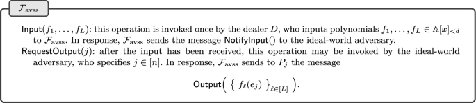
The AVSS ideal functionality (parameterized by n, d, L, $\mathbb {A}$, $\varvec{e}$, and D)

Intuitively speaking, the completeness property for an AVSS protocol says that if an honest dealer D inputs a value or if any honest party output a value, then eventually, all honest parties output a value. Here, “eventually” means if and when all messages sent between honest parties have been delivered. Thus, completeness is not an unconditional guarantee: in the asynchronous communication setting, we formally leave the scheduling of message delivery entirely to the adversary, who may decide to deliver messages sent between honest parties in an arbitrary order, or may choose not to deliver some of them at all.

Turning the above intuitive definition of completeness into a formal one is fairly straightforward. One simply defines an attack game in which the adversary (who controls the corrupt parties and the scheduling of message delivery) wins the game if he can drive the protocol to a state which violates the stated completeness condition, that is, a state such that:

• (i) an honest dealer D has input a value or some honest party has output a value,

• (ii) all messages sent between honest parties have been delivered, and

• (iii) some honest party has not output a value.

Completeness means that any efficient adversary wins this game with negligible probability.

This simple notion of completeness will be sufficient for our purposes. Note that one technical limitation of this definition is that it is only meaningful if the message complexity (that is, the total number of messages sent by any honest party to any other party) is uniformly bounded (that is, bounded by a polynomial that is independent of the adversary, at least with overwhelming probability). Indeed, the completeness property is vacuously satisfied by any protocol in which there are always more messages that need to be delivered (so condition (ii) in the previous paragraph can never be attained). Fortunately, all of the protocols we shall consider here have a uniformly bounded message complexity.

Our approach to modeling completeness closely adheres to the approach introduced in [17]. We note that the related work [20] studies AVSS and AMPC protocols in the UC framework, but makes use of a formal notion of time introduced in [35] to model completeness. Our view is that this extra (and somewhat complicated) machinery is unnecessary and, moreover (echoing the view of [33]), that notions such as liveness and related notions such as completeness are more simply and quite adequately modeled as properties of concrete protocols (as we have done so here) rather than as security properties captured by ideal functionalities.

2.4 Higher-Level Secret Sharing Interfaces

Our ideal functionality $\mathcal {F}_{\textrm{avss}}$ essentially matches that in [20], and models a rather minimalistic, low-level interface. As given, the dealer inputs polynomials over $\mathbb {A}$ and parties receives shares. However, there are no interfaces for encoding a secret value as a polynomial, or for performing various operations on shares, such as opening shares, combining shares to reconstruct a secret, or performing linear operations on sharings.

Our choice of this minimalistic interface is intentional, as it is simple and sufficient for our immediate needs. However, higher-level interfaces can easily be implemented on top of it using standard techniques. For example, the standard way to encode a secret $s \in \mathbb {A}$ as a polynomial is to make s the constant term of the polynomial and choose the other coefficients at random. Doing this, the secret is essentially encoded as the value of the polynomial at the evaluation coordinate 0. For this to work, we require that $(0,e_1,\ldots ,e_n)$ is an exceptional sequence. If this requirement is satisfied, and if $d > t$, then we know that the shares leaked to the adversary reveal no information about the secret s. Moreover, if $n \ge d+2t$, we know we can reconstruct the polynomial, and hence the secret, using a protocol based on “online error correction” (originating in [5], but see [19] for a nice exposition of this and many other related protocols in the asynchronous setting). However, this is not the only mechanism that may be used to encode a secret. For example, one may in fact encode the secret as the leading coefficient, rather than the constant term—while this alleviates the requirement of extending the vector of evaluation coordinates to $n+1$ elements, it may not be convenient in some applications. As another example, with “packed” secret sharing, several secrets may be encoded in a polynomial, by encoding these secrets at different evaluation coordinates [29]—while this can improve the performance of some higher-level protocols, it also reduces the resiliency of such protocols.

Also observe that our minimalistic interface also requires that the ring $\mathbb {A}$ already has appropriate evaluation coordinates. In some applications, the secret may lie in some ring $\mathbb {S}$ that does not contain a large enough exceptional sequence. For example, $\mathbb {S}$ may be a finite field $\mathbb {F}_q$ where q is very small, or a ring such as ${\mathbb {Z}}/(p^k)$, where p is very small. In this case, the standard technique is to secret share over a larger ring $\mathbb {A}\supseteq \mathbb {S}$—for example, a field extension in the case $\mathbb {S}=\mathbb {F}_q$ or a Galois ring extension in the case $\mathbb {S}={\mathbb {Z}}/(p^k)$. Note that a direct application of this technique allows a corrupt dealer to share a secret that lies in $\mathbb {A}\setminus \mathbb {S}$. In some applications, this may be acceptable, while in others, it may not. In Sect. 6, we show how our basic AVSS protocol for secret sharing over $\mathbb {A}$ can be extended to enforce the requirement that secrets do in fact lie in the subring $\mathbb {S}$.

2.5 The Number of Roots of a Polynomial

The following result is standard. Since it is typically proved with respect to fields, for completeness, we give a proof here with respect to rings.

Lemma 2.1

(Schwartz–Zippel over rings) Let $\mathbb {A}$ denote a commutative ring with identity and let $P \in \mathbb {A}[x_1,x_2,\ldots ,x_n]$ be a nonzero polynomial of total degree $\mathfrak {d} \ge 0$. Let $\mathcal {E}\subseteq \mathbb {A}$ be an exceptional set, and let $r_1,\ldots ,r_n$ be selected uniformly, and independently, from $\mathcal {E}$. Then

$$\begin{aligned} \Pr [~ P(r_1,\ldots ,r_n) = 0 ~ ] \le \frac{\mathfrak {d}}{|\mathcal {E}|}. \end{aligned}$$

Proof

We first consider the case of univariate polynomials. Let $f \in \mathbb {A}[x]$ be of degree $\mathfrak {d}$. We show that it can only have at most $\mathfrak {d}$ roots in $\mathcal {E}$. This is done by induction, with the base case of $\mathfrak {d}=0$ being trivial. Now suppose f(x) is of degree $\mathfrak {d}+1$, and the result is true for polynomials of degree $\mathfrak {d}$. We work by contradiction and assume that f(x) has $\mathfrak {d}+2$ distinct roots in $\mathcal {E}$, which we label $r_1,\ldots ,r_{\mathfrak {d}+2}$. We can write $f(x) = (x-r_{\mathfrak {d}+2}) \cdot g(x)$ for some polynomial g(x) of degree $\mathfrak {d}$. Since the roots come from an exceptional set we know that $r_i -r_{\mathfrak {d}+2}$ is invertible for every $i =1,\ldots ,\mathfrak {d}+1$. Hence $r_1,\ldots ,r_{\mathfrak {d}+1}$ must be roots of g(x), and so g(x) has $\mathfrak {d}+1$ distinct roots. This contradicts the inductive hypothesis.

We now prove the main result for multivariate polynomials by induction on n, where the base case of $n=1$ is the univariate case we just considered. So we assume the statement holds for $n \ge 1$, and consider the case of multivariate polynomial with $n+1$ variables $f(x_1,\ldots ,x_{n+1})$. We can write

$$\begin{aligned} f(x_1,\ldots ,x_n) = \sum _{i \le \mathfrak {d}} x_{n+1}^i \cdot f_i(x_1,\ldots ,x_n) \end{aligned}$$

where $f_i$ is a multivariate polynomial in n variables. Since $f(x_1,\ldots ,x_{n+1})$ is not identically zero there is at least one $f_i(x_1,\ldots ,x_n)$ which is not identically zero. Let $\mathfrak {d}'$ denote the largest such index i. We have $\deg (f_{\mathfrak {d}'}) \le \mathfrak {d}-\mathfrak {d}'$ since f has degree at most $\mathfrak {d}$.

We know, by the inductive hypothesis, that for randomly chosen $r_1,\ldots ,r_n \in \mathcal {E}$.

$$\begin{aligned} \Pr [~ f_{\mathfrak {d}'}(r_1,\ldots ,r_n) = 0 ~] \le \frac{\mathfrak {d}-\mathfrak {d}'}{|\mathcal {E}|}, \end{aligned}$$

Now if $f_{\mathfrak {d}'}(r_1,\ldots ,r_n) \ne 0$ then $f(r_1,\ldots ,r_n,x_{n+1})$ is a nonzero univariate polynomial of degree $\mathfrak {d}'$. So by the base case we have, for randomly chosen $r_{n+1} \in \mathcal {E}$,

$$\begin{aligned} \Pr [~ f(r_1,\ldots ,r_n,r_{n+1}) = 0 ~ | ~ f_{\mathfrak {d}'}(r_1,\ldots ,r_n) \ne 0 ~] \le \frac{\mathfrak {d}'}{|\mathcal {E}|}. \end{aligned}$$

By Bayes’ Theorem, and some manipulation, we therefore have

$$\begin{aligned} \Pr [~ f(r_1,\ldots ,r_n,r_{n+1}) = 0 ~ ] \le \frac{\mathfrak {d}-\mathfrak {d}'}{|\mathcal {E}|}+\frac{\mathfrak {d}'}{|\mathcal {E}|} = \frac{\mathfrak {d}}{|\mathcal {E}|}. \end{aligned}$$

$\square$

3 Subprotocols

In this section, we review the subprotocols that our new AVSS protocol will need. Here and throughout the rest of this paper, we assume a network of n parties $P_1, \ldots , P_n$, of which at most $t < n/3$ of them may be statically corrupted, and which are connected by secure point-to-point channels (providing both privacy and authentication). We also assume network communication is asynchronous.

3.1 Random Beacon

A random bacon is a protocol in which each party initiates the protocol and outputs a common value $\omega$ that is effectively chosen at random from an output space $\varOmega$. Such a protocol should satisfy the following security properties (informally stated):

Correctness:

All honest parties that output a value output the same value $\omega$.

Privacy:

The adversary learns nothing about $\omega$ until at least one honest party initiates the protocol.

These security properties are best defined in terms of the ideal functionality $\mathcal {F}_{\textrm{Beacon}}$, which is given in Fig. 2. Note that in $\mathcal {F}_{\textrm{Beacon}}$, a party $P_j$ initiates the protocol by explicitly supplying the input $\textsf {init}$.

Fig. 2

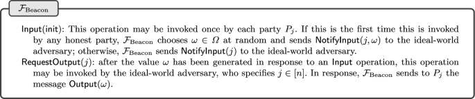
The random beacon functionality $\mathcal {F}_{\textrm{Beacon}}$ (parameterized by output space $\varOmega$)

We also want such a protocol to satisfy the following completeness property: if all honest parties initiate the protocol, then eventually, all honest parties output a value. Just as in Sect. 2.3.1, “eventually” means if and when all messages sent between honest parties have been delivered.

While our main AVSS protocol relies on a random beacon, we will also give a simpler AVSS protocol (in Sect. 7) that does not need a random beacon at all, but instead is analyzed in the random oracle model. But even in our main AVSS protocol, we only need to run one instance of a random beacon protocol to distribute shares of a large batch of polynomials. As such, a random beacon can, in principle, be securely realized with any (not very efficient) protocol without impacting the overall amortized cost of the AVSS protocol (at least for a sufficiently large batch size).

3.1.1 Implementing a Random Beacon

One could implement a random beacon using a $(t+1)$-out-of-n threshold BLS signature scheme [7, 9, 38]. Despite being based on “heavyweight” cryptography, this beacon may be efficient enough for use in our AVSS protocol as well as other applications. However, this beacon requires a hardness assumption that is not post-quantum secure, as well additional setup assumptions (including some kind of distributed key distribution step).

Very recently, [4] showed how to implement a random beacon using just “lightweight” cryptography and no setup assumptions (other than secure channels). Although the communication complexity of their HashRand protocol is super-linear, it is likely good enough for use in our AVSS protocol as well as other applications.

Consider a long-running system in which we will need an unlimited supply of random beacons. Suppose we prepare a sufficiently large initial batch I of beacons, using a protocol such as HashRand. Then we can in fact prepare an unlimited supply of beacons, with a linear amortized communication cost per beacon, as follows. We use the standard technique of having each party generate a batch of sharings of a random secret, agreeing on a set of such batches using a consensus protocol, and then adding up the batches in the set to obtain a batch of sharings of random secrets that are unknown to any party. In fact, we can obtain a linear number of such batches in one go by using well-known “batch randomness extraction” techniques (see [31]). The result of this step is one very large batch J of sharings of secrets that are unknown to any party. Each sharing in the batch J can now be used as a random beacon, by just opening the sharing when it is time to reveal the beacon. The construction of J requires an AVSS protocol and a consensus protocol. We could use our new AVSS protocol, which may or may not require a beacon (depending on the version used), and an efficient consensus protocol such as FIN [24], which definitely requires a beacon. With these protocols, so long as I is sufficiently large to run them, we can make J arbitrarily large in relation to I. So we can arrange that $|J | \gg |I |$, and then partition J into two batches $I'$ and $J'$, where $|I' | = |I |$. Then we can use the batch $J'$ for applications and the batch $I'$ to repeat the process again. The amortized communication complexity per sharing of our AVSS protocol is linear. Although we have to run it a linear number of times per beacon, by using the batch randomness extraction technique, the amortized communication complexity per beacon is still linear. Thus, except for an initial “bootstrapping phase”, we can prepare an unlimited supply of beacons with a linear amortized communication cost per beacon.

Note that while the technique in the previous paragraph allows to prepare batches of random beacons with a linear amortized communication cost per beacon, the communication cost to reveal one beacon is quadratic. There are batching techniques that allow one to reveal many such beacons at once at lower cost (see, for example, Section III of [19]), but it is not clear if this type of batching has many useful applications.

3.1.2 Extending the Output Space of a Random Beacon

Suppose we have a protocol $\varPi$ that securely realizes a random beacon with output space $\varOmega$. We can use $\varPi$ to securely realize a random beacon with a larger output space. One way to do this is to run N instances of $\varPi$ concurrently and concatenate the outputs. This immediately yields a protocol that securely realizes a random beacon with output space $\varOmega ^N$.

Of course, the approach in the previous paragraph comes at a significant cost. A more practical approach is to use a cryptographic pseudorandom generator $G: \varOmega \rightarrow \varOmega '$. If $\varOmega$ is sufficiently large (so that $1/|\varOmega |$ is negligible), and if we model G as a random oracle, then the protocol $\varPi '$ that runs $\varPi$ to obtain the output $\omega \in \varOmega$ and then outputs $\omega ' {:}{=}G(\omega ) \in \varOmega '$ securely realizes a random beacon with output space $\varOmega '$. Indeed, in the random oracle model, a simulator that is given an output $\omega '\in \varOmega '$ of the ideal functionality for the $\varOmega '$-beacon can generate $\omega \in \varOmega$ at random and program the random oracle representing G so that $G(\omega ) = \omega '$.

The above security proof relied heavily on the ability to program the random oracle representing G. If instead of modeling G as a random oracle, we just assume that G is a secure pseudorandom generator, then the above security proof falls apart, and in fact, protocol $\varPi '$ will not securely realize a random beacon. However, the output of $\varPi '$ will still have properties (such as unpredictability) that may be useful in certain applications. The typical setting where this works is one where the security analysis requires a certain failure event $\mathcal {E}$ to occur with negligible probability for randomly chosen $\omega '\in \varOmega '$, and the occurrence of $\mathcal {E}$ can be detected efficiently as a function of $\omega '$ and data that are available to the adversary prior to invoking protocol $\varPi$.

3.2 Reliable Broadcast

A reliable broadcast protocol allows a sender S to broadcast a single message m to $P_1, \ldots , P_n$. Such a protocol should satisfy the following security property (informally stated):

Correctness:

All honest parties that output a message must output the same message. Moreover, if the sender S is honest, that message is the one input by S.

This security property is best defined in terms of the ideal functionality $\mathcal {F}_{\textrm{ReliableBroadcast}}$, which is given in Fig. 3.

We also want such a protocol to satisfy the following completeness property: if an honest sender S inputs a message or if any honest party outputs a message, then eventually, all honest parties output a message. As usual, “eventually” means if and when all messages sent between honest parties have been delivered.

Fig. 3

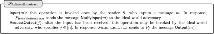
The reliable broadcast ideal functionality (parameterized by S)

Fig. 4

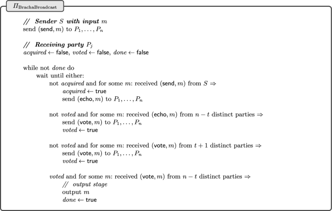
Bracha’s protocol for reliable broadcast

3.2.1 Bracha Broadcast

A simple reliable broadcast protocol is called Bracha Broadcast [11] and is given in Fig. 4. We express the logic for the sender as a separate process, even though the sending party is also one of the receiving parties. First note, that the communication complexity of Bracha broadcast is clearly $O(n^2 \cdot |m |)$.

Since we will be using variants of Bracha broadcast later, we highlight some important properties of the echo/vote logic of this protocol. Suppose that there are $t' \le t$ corrupt parties.

Bracha Property B0:

If an honest party receives $n-t$ votes for the same message, then all honest parties will eventually vote for some message.

Suppose an honest party receives $n-t$ votes for the same message. Then at least $n-2t \ge t+1$ honest parties must have voted for this message. Upon receipt of these $t+1$ votes, each honest party will vote if they have not done so already.

Bracha Property B1:

If an honest sender S inputs a message, then all honest parties will eventually vote for some message.

Eventually, all honest parties will echo the sender’s message, unless some honest party enters the output stage without doing so. In the former case, upon receipt of these echoes, each honest party will vote if they have not already done so. In the latter case, some honest party must have received $n-t$ votes on the same message, and the property follows from Bracha Property B0.

Bracha Property B2:

If an honest party votes for a message, then at least $n-t-t'$ honest parties must have echoed the same message.

This is because the very first time any honest party votes for a given message it must be the case that this party received $n-t$ echoes on that message from distinct parties, of which $n-t-t'$ must be honest.

Bracha Property B3:

If two honest parties vote for a message, they must vote for the same message.

This is because if two honest parties vote different messages, then by Bracha Property B2 we have one set of $n-t-t'$ honest parties echoing one message, and a second, disjoint set of $n-t-t'$ honest parties echoing a different message, which means $2(n-t-t') \le n-t'$, which implies $n \le 2t+t' \le 3t$.

The correctness property of Bracha broadcast easily follows from Bracha Properties B2 and B3 (B3 implies all honest parties must output the same message, and B2 implies that if the sender is honest, this message must be the one input by the sender). The completeness properties easily follows from Bracha Properties B0, B1, and B3. Since, B0 and B1 imply that if an honest sender inputs a message or an honest party outputs a message, then all honest parties eventually vote for a message, and B3 says they all vote for the same message, which implies all honest parties eventually output a message.

3.2.2 Compact Broadcast

The communication complexity of Bracha broadcast can be improved by the use of erasure codes. To this end, we need an $(n,n-2t)$ erasure code, which has the following properties: a message m can be efficiently encoded as a vector of n fragments $(f_1, \ldots , f_n)$ in such a way that m can be efficiently reconstructed (decoded) from any subset of $n-2t$ fragments. An $(n, n-2t)$-Reed-Solomon code can be used for this purpose, but other constructions are possible as well. In any reasonable construction, the size of each fragment will be about $|m |/(n-2t)$.

We can use such an erasure code to build a reliable broadcast protocol with better communication complexity as follows. Given a long message m, the sender S encodes the message using an $(n, n-2t)$ erasure code, to obtain a vector of n fragments $(f_1, \ldots , f_n)$. Each fragment has size roughly $|m |/(n-2t)$ — so assuming $n > 3t$, the size of each fragment is at most roughly $3 |m | / n$. The sender S then sends each fragment $f_j$ to party $P_j$, who then echoes that fragment to all other parties. Each party can then collect enough fragments to reconstruct m. To deal with dishonest parties, some extra steps must be taken.

This approach was initially considered in [21], who give a protocol with communication complexity $O(n \cdot |m | + \lambda \cdot n^2 \cdot \log n )$. Here, $\lambda$ is the output length of a collision-resistant hash function. The factor $\log n$ arises from the use of Merkle trees. If $|m | \gg \lambda \cdot n \cdot \log n$, this is essentially optimal—indeed, any reliable broadcast protocol must have communication complexity $\varOmega (n \cdot |m |)$, since every party must receive m.

Recall that that a Merkle tree allows one party, say Charlie, to commit to a vector of values $(v_1, \ldots , v_k)$ using a collision resistant hash function by building a binary tree whose leaves are the hashes of $v_1, \ldots , v_k$, and where each internal node of the tree is the hash of its (at most two) children. The root r of the tree is the commitment. Charlie may “open” the commitment at an index $i \in [k]$ by revealing $v_i$ along with a “validation path” $\pi _i$, which consists of the siblings of all nodes along the path in the tree from the hash of $v_i$ to the root r. We call $\pi _i$ a validation path for $v_i$ under r at i. Such a validation path is checked by recomputing the nodes along the corresponding path in the tree, and testing that the recomputed root is equal to the given commitment r. The collision resistance of the hash function ensures that Charlie cannot open the commitment to two different values at a given index.

We give here the details of a reliable broadcast protocol that is based on erasure codes and Merkle trees, and which achieves the same communication complexity as that in [21]. This protocol is similar to that presented in  [21], but is a bit simpler and also bears some resemblance to a related protocol in the DispersedLedger system  [40]. Our reasons for presenting this protocol are threefold: first, to make this paper more self contained; second, because this protocol has somewhat better communication complexity than the one in [21]; and third, because later in this paper, we will modify this protocol to achieve other goals. We call this reliable broadcast protocol $\varPi _{\textrm{CompactBroadcast}}$ and it is given in Fig. 5.

Fig. 5

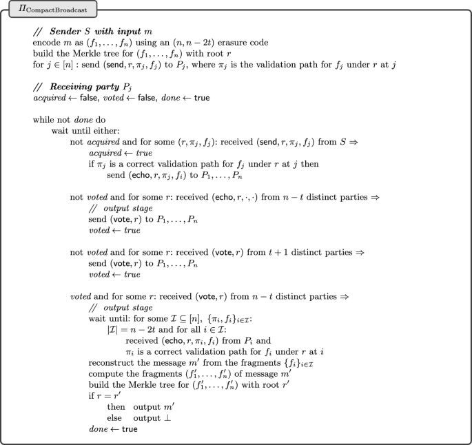
A reliable broadcast protocol based on erasure codes and Merkle trees

The reader may observe that $\varPi _{\textrm{CompactBroadcast}}$ has essentially the same structure as Bracha’s reliable broadcast protocol, where the message being broadcast is the root of a Merkle tree. The correctness property of $\varPi _{\textrm{CompactBroadcast}}$ follows from Bracha Properties B2 and B3, and the collision resistance of the hash function used for building the Merkle trees. The completeness property of $\varPi _{\textrm{CompactBroadcast}}$ follows from Bracha Properties B0, B1, B2 and B3. Specifically, Bracha Property B2 in this context ensures that in $\varPi _{\textrm{CompactBroadcast}}$, if any honest party votes for a root r, then at least $n-2t$ honest parties must have echoed r along with a corresponding validation path and fragment, so that all honest parties will eventually be able to reconstruct a message from these $n-2t$ fragments in the output stage.

3.2.3 Other Reliable Broadcast Protocols

For somewhat shorter messages, a protocol such as that in [25] may be used, which achieves a communication complexity of $O(n \cdot |m | + \lambda \cdot n^2 )$. The protocol $\varPi _{\textrm{CompactBroadcast}}$ above uses only an erasure code, while the protocol in [25] requires an “online” error correcting code, which may be more computationally expensive than erasure codes. Another potential advantage of $\varPi _{\textrm{CompactBroadcast}}$ over the protocol in [25] is that the former has a very balanced communication pattern, which can be important to prevent a communication bandwidth bottlenecks. The paper [26] improves on [25], obtaining the same communication complexity, but with a balanced communication pattern.

3.2.4 Relation to AVID

The design of $\varPi _{\textrm{CompactBroadcast}}$ is based on the notion of Asynchronous Verifiable Information Dispersal, or AVID. In an AVID protocol, a sender S wants to send a message m to some or possibly all of the parties $P_1, \ldots ,P_n$. There are two phases to such a protocol: the dispersal phase, where S disperses m (or fragments of m) among $P_1, \ldots ,P_n$, and the retrieval phase, where individual $P_j$’s may retrieve m. The correctness property for such a protocol is essentially the same as that of a reliable broadcast protocol:

All honest parties that output a message in the retrieval phase output the same message. Moreover, if S is honest, that message is m.

The completeness property has two parts. First, in the dispersal phase:

If an honest sender S inputs a message or if one honest party completes the dispersal phase, then every honest party eventually completes the dispersal phase.

Second, in the retrieval phase:

If the dispersal phase has completed (for some honest parties), and the retrieval phase for an honest party $P_j$ is initiated, then $P_j$ eventually outputs a message.

Note that one can use any AVID protocol to implement reliable broadcast, by first dispersing the message and then having every party retrieve the message.

The point of using an AVID protocol is that in situations where only a small number of parties need to retrieve the message, communication complexity can be much lower than in a reliable broadcast protocol. For example, the dispersal phase of the AVID protocol in the DispersedLedger system [40] is very similar to our protocol $\varPi _{\textrm{CompactBroadcast}}$, except that the echo messages in the former do not include the validation paths and fragments—rather, these data are only disseminated to those parties that actually need to retrieve the message. The resulting AVID protocol thus has a communication complexity of $O(|m | + \lambda \cdot n^2)$ in the dispersal phase and $O(|m | + \lambda \cdot n \cdot \log n)$ per retrieval.

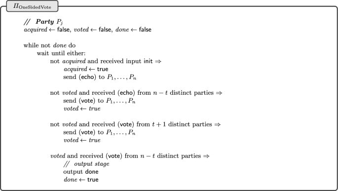
3.2.5 One-Sided Voting

A degenerate version of Bracha broadcast can be used as a simple one-sided voting protocol, see Fig. 6. In this protocol, each party may initiate the protocol and may output the value done. The key security property of this protocol (informally stated) is as follows:

Correctness:

If any honest party outputs $\textsf {done}$, then at least $n-t-t'$ honest parties initiated the protocol, where $t' \le t$ is the number of corrupt parties.

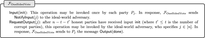
This security property is best defined in terms of the ideal functionality $\mathcal {F}_{\textrm{OneSidedVote}}$, which is given in Fig. 7. Note that in $\mathcal {F}_{\textrm{OneSidedVote}}$, a party $P_j$ initiates the protocol by explicitly supplying the input $\textsf {init}$.

This protocol also satisfies the following completeness property: if all honest parties initiate the protocol or some honest party outputs $\textsf {done}$, then eventually, all honest parties output done. As usual, “eventually” means if and when all messages sent between honest parties have been delivered.

The correctness property follows from the analog of Bracha Property B2. The completeness property follows from the analogs of Bracha Properties B0 and B1.

Fig. 6

Degenerate version of Bracha’s protocol for one-sided voting

Fig. 7

The one-sided voting ideal functionality $\mathcal {F}_{\textrm{OneSidedVote}}$

3.3 Secure Message Distribution

We require a new type of protocol, which we call a secure message distribution protocol. Such a protocol enables a sender S to securely distribute a vector $\textbf{m}= (m_1, \ldots , m_n)$ of messages, so that during an initial distribution phase, each party $P_j$ outputs $m_j$. After receiving its own message $m_j$, party $P_j$ may optionally forward this message to another party. Moreover, after receiving any message $m_u$ (either its own or one forwarded to it), party $P_j$ may optionally forward $m_u$ to another party. This forwarding functionality will be needed to deal with the “unhappy” path of our AVSS protocol.

Such a protocol should satisfy the following security properties (informally stated):

Correctness:

If any honest parties produce an output in the distribution or forwarding phases, those messages must be consistent with a message vector $\textbf{m}=(m_1,\ldots ,m_n)$—that is, the message output by honest $P_j$ during the distribution phase must be $m_j$, and any message output by some honest party during the forwarding phase as ostensibly belonging to to some party $P_{u}$ must be $m_{u}$. Moreover, if the sender S is honest, $\textbf{m}$ must be the same message vector input by S.

Privacy:

If the sender S and party $P_{u}$ are honest, and no honest party forwards $m_{u}$ to a corrupt party, then the adversary learns nothing about $m_{u}$.

Note that whenever a party outputs a message (in either the distribution or forwarding phase), that message may be $\bot$, which can only happen if the sender is corrupt.

It will also be convenient for us to allow a party to include an identifying tag along with the forwarded message.

We may more precisely formulate the security properties for secure message distribution as the ideal functionality $\mathcal {F}_{\textrm{SecMsgDst}}$, which is given in Fig. 8. We note that $\mathcal {F}_{\textrm{SecMsgDst}}$ also captures an input extractability property that intuitively means that a corrupt sender S must explicitly commit to a vector of all input messages before any honest party outputs its own message in the distribution phase (or any forwarded message for that matter). This is a property that will be essential in the security analysis of our AVSS protocol.

We bring to the reader’s attention the logic in the ideal functionality $\mathcal {F}_{\textrm{SecMsgDst}}$ for processing a request by a party $P_j$ to forward a message $m_u$ to another party. The logic enforces a precondition that requires that either (i) the message to be forwarded is one that $P_j$ has already received (either its own or one forwarded to it), or (ii) $P_j$ and S are both corrupt. In any implementation, an honest party will always simply ignore an input that requests it to forward a message it does not have. If we did not have such a precondition, an ideal-world adversary could trivially circumvent the privacy property by having a corrupt $P_j$ simply ask the ideal functionality to forward a message $m_u$ belonging to an honest party $P_u$ to itself or to some other corrupt party.

In fact, $\mathcal {F}_{\textrm{SecMsgDst}}$ is a bit stronger than we need, in the sense that we may assume that when the sender S is honest, no honest $P_j$ will forward its message $m_j$ to any other party. As we will see, this constraint will be satisfied by our AVSS protocol. In the UC framework, this can be captured by only considering restricted environments that satisfy this constraint. We will give an efficient protocol that securely realizes $\mathcal {F}_{\textrm{SecMsgDst}}$ with respect to such constrained environments. As we will also see, in the random oracle model, essentially the same protocol is secure even without this constraint.

Fig. 8

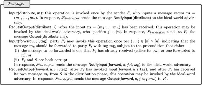
The ideal functionality for secure message delivery $\mathcal {F}_{\textrm{SecMsgDst}}$ (parameterized by S)

We also want a secure message distribution protocol to satisfy the following completeness property, which has two parts. First, in the distribution phase:

If an honest sender S inputs a vector of messages, or if one honest party outputs a message in the distribution phase, then eventually, all honest parties output a message in the distribution phase.

Second, in the forwarding phase:

If an honest party $P_j$ forwards a message $m_u$ to an honest party $P_i$, then eventually, $P_i$ receives $m_u$.

As usual, “eventually” means if and when all messages sent between honest parties have been delivered.

In Sect. 4 we give a secure message distribution protocol that is built from “lightweight” cryptographic primitives, specifically, semantically secure symmetric key encryption and a hash function. The hash function needs to be collision resistant and to also satisfy a kind of related-key indistinguishability assumption (see Sect. 4.2 for more details). The communication complexity of the distribution phase of our protocol is $O(|\textbf{m} | + \lambda \cdot n^2\cdot \log n )$. If an honest party forwards a message $m_{u}$ to another party, this adds $O(|m_{u} | + \lambda \cdot n\cdot \log n )$ to the communication complexity.

In our application to AVSS, we will only use the forwarding mechanism on the “unhappy path”, in which a corrupt sender provably misbehaves. In particular, unless we are on the “unhappy path”, the forwarding mechanism will not contribute to the communication complexity at all.

4 Building Secure Message Distribution

In this section we show how to implement the secure message distribution functionality from Sect. 3.3. Note that [39] and [30] show how to implement this type of functionality using “heavyweight” cryptographic primitives based on discrete logarithms. In particular, [30] rigorously defines a particular multi-encryption primitive with an appropriate notion of chosen ciphertext security and a verifiable decryption protocol and presents practical constructions that are provably secure in the random oracle model.

While such constructions may well yield acceptable performance in practice, we show here that one can implement this functionality using only “lightweight” cryptographic primitives. The resulting protocols are certainly more efficient than those based on discrete logarithms and also have the advantage of providing post-quantum security.

4.1 Reliable Message Distribution

We start out by considering the simpler notion of a reliable message distribution protocol, which satisfies all the properties of a secure message secure message distribution protocol except privacy.

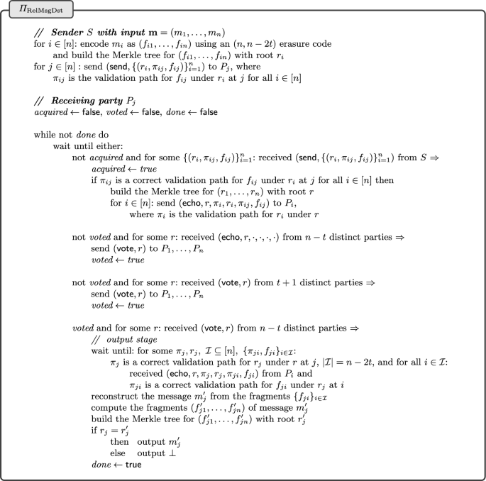
We implement this using a variant of the reliable broadcast protocol $\varPi _{\textrm{CompactBroadcast}}$ in Sect. 3.2. In the distribution phase, the sender S starts with a vector of messages $\textbf{m}=(m_1,\ldots ,m_n)$; it encodes each $m_i$ as a vector of fragments $(f_{i1}, \ldots ,f_{i n})$ and then builds a Merkle tree for $(f_{i1}, \ldots ,f_{i n})$ with root $r_i$; it then sends each $P_j$ the collection of values $\{ (r_i, \pi _{ij}, f_{ij}) \}_{i=1}^n$, where each $\pi _{ij}$ is the validation path for $f_{ij}$ under $r_i$ at j. Thus, each $P_j$ receives the jth fragment of all n messages. An echo message from $P_j$ to $P_i$ now includes $r, \pi _i, r_i, \pi _{ij}, f_{ij}$, where r is the root of the Merkle tree built from $(r_1,\ldots ,r_n)$ and $\pi _i$ is the validation path for $r_i$ under r at i. The vote messages include just the root r. Once party $P_j$ collects sufficiently many vote messages for a root r, it enters the output stage, and waits to collects sufficiently many echo messages that contain valid fragments of the jth message from which it can reconstruct that message. Details of the complete distribution phase are in Fig. 9.

Fig. 9

The distribution phase of a reliable message distribution protocol

When $P_j$ completes the distribution phase of the protocol, it can optionally forward $m_j$ to another party Q by sending to Q the values it obtained in the last step of the distribution phase, specifically, the values $\pi _j, r_j$ along with the collection of $n-2t$ values $\{ \pi _{ji}, f_{ji} \}_i$. Party Q, who we assume has also completed the distribution phase, can validate this information and compute the message using the same logic used by $P_j$. This validation consists of two parts:

• In the first part, Q checks that the validation paths are correct with respect to the root r acquired when entering the output stage; if this check fails, the forwarding subprotocol fails and no output is delivered.

• In the second part, Q reconstructs the fragments and their Merkle tree, and compares the Merkle tree roots. If this check fails, the forwarding subprotocol outputs $\bot$; otherwise, it outputs the message.

The first part detects if the party forwarding the message is misbehaving, while the second detects if the sender S was misbehaving.

The same logic above can obviously be adapted to allow a party to forward any message that it has received, either its own or one that was forwarded to it.

4.1.1 Correctness and Completeness

The correctness and completeness properties for protocol $\varPi _{\textrm{RelMsgDst}}$ follow from essentially the same argument used in Sect. 3.2.2 for the corresponding properties for protocol $\varPi _{\textrm{CompactBroadcast}}$. Protocol $\varPi _{\textrm{RelMsgDst}}$ also satisfies the input extractability property, which follows from the same argument used in Sect. 3.2.2 for the completeness property for protocol $\varPi _{\textrm{CompactBroadcast}}$. Specifically, Bracha Property B2 ensures that when one honest party reaches the output stage in $\varPi _{\textrm{RelMsgDst}}$, at least $n-2t$ honest parties have echoed validation paths and fragments for all input messages $m_1, \ldots , m_n$. Therefore, assuming collision resistance for the hash function used for building Merkle trees, all these messages are fully determined at this time.

4.1.2 Communication Complexity

The communication complexity of the distribution phase is $O(|\textbf{m} | + \lambda \cdot n^2\cdot \log n )$. If an honest party forwards a message $m_{u}$ to another party, this adds $O(|m_{u} | + \lambda \cdot n\cdot \log n )$ to the communication complexity.

Note that when a corrupt party forwards a message to an honest party, this does not contribute anything to the communication complexity. This property will be important when we analyze the communication complexity of our AVSS protocol on the “happy path”. The reason this type of forwarding does not contribute anything is that in defining communication complexity, we count the number of bits sent by all honest parties to all parties. One might argue that this is a theoretical distinction, and that in practice, one should count all bits sent and received by honest parties. However, such a definition of communication complexity is unworkable, as it cannot be upper bounded at all—corrupt parties may “spam” their honest peers with an unbounded amount of data. In practice, honest parties would likely attempt to distribute their download bandwidth equitably among all of its peers and employ some kind of “spam prevention” strategy to protect itself against peers who try to monopolize its download bandwidth.

4.1.3 Relation to AVID

In Sect. 3.2.4 we briefly recalled the notion of an AVID protocol. In fact, the design of our protocol $\varPi _{\textrm{RelMsgDst}}$ is inspired by the AVID protocol in the DispersedLedger system [40]. In principle, one could build a reliable message distribution protocol simply by running n instances of an AVID protocol concurrently, one for each input message $m_j$: the retrieval mechanism of the AVID protocol could be used both to deliver $m_j$ to $P_j$ and to optionally forward $m_j$ to other parties. So we could have simply implemented this generic strategy using the AVID protocol in [40]. There are several reasons we did not do this:

• This generic strategy, instantiated with DispersedLedger’s AVID protocol, would result in a reliable message distribution protocol whose communication complexity in the distribution phase is $O(|\textbf{m} | + \lambda \cdot n^3)$ rather than $O(|\textbf{m} | + \lambda \cdot n^2\cdot \log n )$. Note that the same communication complexity would result if we instantiated with the AVID protocol in [26].

• This generic strategy, instantiated with DispersedLedger’s AVID protocol, would result in a reliable message distribution protocol where the number of rounds of communication in the distribution phase was 4 rather than 3.

• In this generic strategy, where we use the retrieval mechanism of AVID to implement the forwarding mechanism of reliable message distribution, we run into a subtle problem regarding communication complexity. As noted above, in our reliable message distribution protocol, when a corrupt party forwards its message to an honest party, this does not contribute anything to the communication complexity. However, if we use the retrieval mechanism of AVID for message forwarding, when a corrupt party attempts to forward its message to an honest party, all honest parties must participate in the protocol, which contributes to the communication complexity. So in this case, some additional mechanism would be required to prevent or at least detect misusing the forwarding mechanism.

In addition to the above, we wanted to present a concrete reliable message distribution protocol which we could then easily modify to add data privacy and so obtain a secure message distribution protocol.

4.2 Secure Key Distribution

The above reliable message distribution protocol does not provide any data privacy. This can be remedied by augmenting it with a protocol for secure key distribution and then using these secret keys to encrypt the messages and using $\varPi _{\textrm{RelMsgDst}}$ to distribute the resulting ciphertexts.

We sketch briefly here the properties that a secure key distribution protocol should satisfy and how to build one, and then below in Sect. 4.3, we show in how to integrate this protocol into our protocol $\varPi _{\textrm{SecMsgDst}}$ to obtain a secure message distribution protocol.

In a secure message distribution protocol, the goal is to have the sender S distribute a vector of keys $\varvec{k} = (k_1, \ldots , k_n)$, so that each party $P_j$ obtains $k_j$. Here, if the sender S is honest, the keys $k_1, \ldots , k_n$ are not input by the sender, but rather are generated by the protocol itself, and the sender obtains the vector $\varvec{k}$ as an output of the protocol; however, a corrupt sender S may effectively choose and input an arbitrary vector $\varvec{k}$. In addition, just like for reliable message distribution, the protocol should allow a party to forward a key that it has received to another party. Such a protocol should satisfy analogous correctness and completeness (as well as input extractability) properties. In addition, the following property should hold:

Privacy:

If the sender S and party $P_{u}$ are honest, and no honest party forwards $k_{u}$ to a corrupt party, then the adversary learns nothing about $k_{u}$.

To implement such a scheme, which we call $\varPi _{\textrm{SecKeyDst}}$, we modify the reliable message distribution protocol $\varPi _{\textrm{RelMsgDst}}$ so that instead of encoding a key using an erasure code, we share it using Shamir secret sharing. In more detail, let $H: [0..n] \times F \rightarrow \mathcal {K}$ be a cryptographic hash function, where F is a large finite field and $\mathcal {K}$ is the key space. Let $(\eta _0, \eta _1, \ldots , \eta _n)$ be fixed sequence of distinct elements in F.³

The sender proceeds as follows. For each $i\in [n]$, the sender chooses a random polynomial $\theta _i \in F_{< n-2t}$. Let $s_{ij} {:}{=}\theta _i(\eta _j)$ for $j\in [0..n]$. The key $k_i$ is defined as $k_i {:}{=}H(0,s_{i0})$. The sender builds a Merkle tree from $(\ (H(1,s_{i1}), \ldots , H(n,s_{in}) \ )$ with root $r_i$. and sends to each $P_j$ the collection of values $\{ (r_i, \pi _{ij}, s_{ij}) \}_{i=1}^n$, where $\pi _i$ is a validation path for $H(j, s_{ij})$ under $r_i$ at j.

Upon receiving such a message from S, and validating it is of the correct form, each party $P_j$ then builds a Merkle tree for $(r_1, \ldots , r_n)$ with root r and echoes to each $P_i$ the tuple $(r, \pi _i, r_i, \pi _{ij}, s_{ij})$, where $\pi _i$ is a validation path for $r_i$ under r. The voting logic works just as before. In the output stage, $P_j$ waits for valid echo messages from a set of $n-2t$ distinct parties $P_i$, and then reconstructs a polynomial $\theta '_j \in F[x]_{< n-2t}$ via polynomial interpolation from $\{ s_{ij} \}_{i}$. It then builds a Merkle tree from $(\ H(1,\theta '_j(\eta _1)), \ldots , H(n,\theta _j(\eta _n)) \ )$ with root $r'_j$. If $r_j = r$, it outputs the key $H(0, \theta '_j(0))$, and otherwise outputs $\bot$.

When $P_j$ completes the distribution phase of the protocol, it can optionally forward $k_j$ to another party Q by sending to Q the values it obtained in the last step of the distribution phase, specifically, the values $\pi _j, r_j$ along with the collection of $n-2t$ values $\{ \pi _{ji}, s_{ji} \}_i$. Party Q who can validate this information and compute $k_j$ using the same logic used by $P_j$. This strategy can obviously be adapted to allow a party to forward any key that it has received, either its own or one that was forwarded to it.

We note that $\varPi _{\textrm{SecKeyDst}}$ has some rough similarities to the asynchronous weak VSS protocol in [23], but the goals and a number of details are quite different.

4.2.1 Correctness and Completeness

One can easily adapt the analysis of $\varPi _{\textrm{RelMsgDst}}$ to show that $\varPi _{\textrm{SecKeyDst}}$ satisfies the correctness and completeness (as well as input extractability) properties, assuming the hash function used to implement the Merkle trees, as well as H, are collision resistant.

4.2.2 Proving Privacy Under the Linear Hiding Assumption

To prove the privacy property for $\varPi _{\textrm{SecKeyDst}}$, we make the following assumption on the hash function $H: [0..n] \times F \rightarrow \mathcal {K}$, which we call the linear hiding assumption. This is a kind of indistinguishability assumption under a “related key attack”.

This assumption is defined by a game in which the adversary first chooses a collection of pairs $\{ (a_i, b_i ) \}_{i \in \mathcal {I}}$, where $\mathcal {I} \subseteq [0..n]$ and each $a_i$ is nonzero. The task of the adversary is to distinguish the distribution

$$\begin{aligned} \big \{ H(i, a_i \cdot s + b_i) \big \}_{i \in \mathcal {I}}, \end{aligned}$$

where $s \in F$ is randomly chosen, from the uniform distribution on $\mathcal {K}^\mathcal {I}$. The assumption states that no computationally bounded adversary can effectively distinguish these two distributions.

This assumption is certainly true in the random oracle model, assuming $1/|F |$ is negligible. Indeed, if we model H as a random oracle, the best the adversary can do is evaluate H at many points $(i, s^*)$ for $i \in \mathcal {I}$ and $s^* \in F$, and hope that $s^* = a_i \cdot s + b_i$. So it seems a reasonable assumption.

We can use this assumption to prove the privacy of $\varPi _{\textrm{SecKeyDst}}$ as follows. Assume the sender S is honest and consider any one honest party. For this party, the sender chooses a random polynomial $\theta \in F[x]_{< n-2t}$ and computes $s_{j} {:}{=}\theta (\eta _j)$ for $j\in [0..n]$. Let $\mathcal {C}$ be the set of corrupt parties, which we are assuming is of cardinality $\le t < n-2t$, and let $\mathcal {H}{:}{=}[n] {\setminus } \mathcal {C}$ be the set of honest parties. During the execution of the protocol, the adversary learns $s_{j}$ for $j \in \mathcal {C}$. The only other information about the polynomial $\theta$ that the adversary learns is derived as a function of $H(i, s_{i})$ for $i \in \mathcal {H}$. We want to argue that given this information, the adversary cannot distinguish the actual key $H(0, s_{0})$ from a random key, under the linear hiding assumption.

Without loss of generality, we may give the adversary even more information, namely let $\mathcal {C}' \subseteq [n]$ be an arbitrary set of size exactly $n-2t-1$ containing $\mathcal {C}$, and let us assume that the adversary is given $s_{j}$ for $j \in \mathcal {C}'$ and $H(i, s_{i})$ for $i \in \mathcal {H}' {:}{=}[n] {\setminus } \mathcal {C}'$. By Lagrange interpolation, for each $i \in \mathcal {H}'$, there exist nonzero constants $\{ \lambda _{ij} \}_{j \in \mathcal {C}' \cup \{0\}}$ in the field F such that

$$\begin{aligned} s_{i} = \sum _{j \in \mathcal {C}' \cup \{0\}} \lambda _{ij} \cdot s_{j}. \end{aligned}$$

The indistinguishability of $H(0, s_0)$ from random follows directly from the linear hiding assumption, where in the attack game for that assumption, we use the adversarially chosen pairs

$$\begin{aligned} \{ (a_i, b_i) \}_{i \in \mathcal {H}' \cup \{0\}}, \end{aligned}$$

where

$$\begin{aligned} (a_i, b_i) = {\left\{ \begin{array}{ll} \left( \, \lambda _{i0}, \, \sum _{j \in \mathcal {C}'} \lambda _{ij} \cdot s_{j} \,\right) , &{} \text {if }i \in \mathcal {H}'; \\ (1, 0), &{} \text {if }i=0. \end{array}\right. } \end{aligned}$$

That proves the privacy property of a single honest party’s key. The proof can easily be extended to cover all honest parties’ keys by a standard “hybrid” argument.

We note that the indistinguishability property for keys, and the fact that the key space itself must be large (as we are assuming the key space is the output space of a collision-resistant hash), implies that keys are unpredictable.

4.2.3 Domain Separation Strategies for H

Our construction uses the simple “domain separation” strategy for H, where we include both j and $s_{ij}$ in the input to H. The inclusion of j is not strictly necessary, but it yields a simpler and quantitatively better security analysis in the random oracle model. In fact, if we include i as well in the input, we would obtain an even better concrete security bound (avoiding the “hybrid” argument mentioned above). Moreover, as a practical matter, one should include even more contextual information as an input to H that identifies the individual instance of the protocol, including the identity of the sender. This is not only good security practice, but will also yield better concrete security bounds for a system in which many instances of the protocol are run.

4.2.4 Communication Complexity

Assuming individual keys are of size $O(\lambda )$, the communication complexity of the distribution phase is $O(\lambda \cdot n^2\cdot \log n )$. If an honest party forwards a key to another party, this adds $O(\lambda \cdot n\cdot \log n )$ to the communication complexity. Just as in Sect. 4.1.2, then a corrupt party forwards its key to an honest party, this does not contribute anything to the communication complexity.

4.3 A Secure Message Distribution Protocol

We can build a protocol that securely realizes $\mathcal {F}_{\textrm{SecMsgDst}}$ by using $\varPi _{\textrm{SecKeyDst}}$ to securely distribute secret keys that are used to encrypt messages using any semantically secure symmetric key encryption scheme, and then distributing the resulting ciphertexts using $\varPi _{\textrm{RelMsgDst}}$. In fact, we can integrate the logic of $\varPi _{\textrm{SecKeyDst}}$ directly into $\varPi _{\textrm{RelMsgDst}}$, so that there is just a single root r that controls both keys and ciphertexts. The distribution phase of the resulting protocol $\varPi _{\textrm{SecMsgDst}}$ is given in Fig. 10. Here, $c \leftarrow \textsf{Encrypt}(k,m)$ encrypts the message m under the key k, producing the ciphertext c, and $m \leftarrow \textsf{Decrypt}(k, c)$ performs the corresponding decryption.

Fig. 10

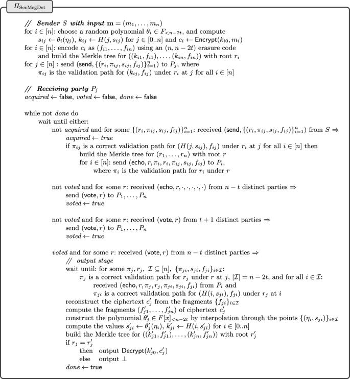
The distribution phase of a secure message distribution protocol

When $P_j$ completes the distribution phase of the protocol, it can optionally forward $m_j$ to another party Q by sending to Q the values it obtained in the last step of the distribution phase, specifically, the values $\pi _j, r_j$ along with the collection of $n-2t$ values $\{ \pi _{ji}, s_{ji}, f_{ji} \}_i$. Party Q who can validate this information and compute $m_j$ using the same logic used by $P_j$. This strategy can obviously be adapted to allow a party to forward any message that it has received, either its own or one that was forwarded to it.

The same comments on domain separation for H in Sect. 4.2.3 apply here as well.

We note that it may seem that the two-step approach of dispersing secret keys, and then dispersing encrypted messages is superfluous. However, this is essential to get good communication complexity by taking advantage of the fact that secret keys are much shorter than messages.

4.3.1 Security and Completeness

If $\varPi _{\textrm{SecMsgDst}}$ securely realizes the $\mathcal {F}_{\textrm{SecMsgDst}}$ functionality, then it will surely satisfy the corresponding correctness and privacy (as well as input extractability) properties. In the security analysis of our AVSS protocol, we will want to work directly with the $\mathcal {F}_{\textrm{SecMsgDst}}$ functionality, rather than with these specific security properties (which are anyway too informal).

Recall from Sect. 3.3 the notion of a restricted environment, which is an environment in the UC framework that never instructs an honest party to forward its own message when S is honest. Such restricted environments are actually sufficient for our AVSS application.

It is straightforward to show that if

• H and the hash function used for building Merkle trees are collision resistant,

• H satisfies the linear hiding assumption, and

• the encryption scheme used to encrypt messages is semantically secure

then protocol $\varPi _{\textrm{SecMsgDst}}$ securely realizes $\mathcal {F}_{\textrm{SecMsgDst}}$ with respect to restricted environments.

It is also straightforward to show that if H and the hash function used for building Merkle trees are collision resistant, then $\varPi _{\textrm{SecMsgDst}}$ satisfies the completeness property for secure message distribution.

One can in fact prove that $\varPi _{\textrm{SecMsgDst}}$ securely realizes $\mathcal {F}_{\textrm{SecMsgDst}}$ without restriction under the same assumptions on the hash functions, but where the encryption scheme is built using a random oracle to make it “equivocable”—namely, where we define $\textsf{Encrypt}(k,m) {:}{=}\textit{hash}(k) \oplus m$, and model $\textit{hash}$ as a random oracle. We also speculate that under these assumptions, $\varPi _{\textrm{SecMsgDst}}$ securely realizes $\mathcal {F}_{\textrm{SecMsgDst}}$ under adaptive corruptions (although we have not worked out the details of this).

4.3.2 Communication Complexity

The communication complexity of the distribution phase is $O(|\textbf{m} | + \lambda \cdot n^2\cdot \log n )$. If an honest party forwards a message $m_{u}$ to another party, this adds $O(|m_{u} | + \lambda \cdot n\cdot \log n )$ to the communication complexity. Just as in Sect. 4.1.2, when a corrupt party forwards a message to an honest party, this does not contribute anything to the communication complexity.

5 Our AVSS Protocol

We now present and analyze our new AVSS protocol. This is a generic protocol which works over an arbitrary ring. We will show how to instantiate it over finite fields and Galois rings. As will see, different instantiations lead to different failure bounds in the analysis.

5.1 Description of the Protocol

Notation is as in Sect. 2; specifically, we have a finite commutative ring $\mathbb {A}$ and a vector of evaluation coordinates $\varvec{e} = (e_1, \ldots , e_n) \in \mathbb {A}^n$ that forms an exceptional sequence, that is, we have $e_i - e_j \in \mathbb {A}^*$ for all $i \ne j$.

As usual, we assume a network of n parties $P_1, \ldots , P_n$, of which at most $t < n/3$ of them may be statically corrupted, and which are connected by secure point-to-point channels (providing both privacy and authentication). We also assume network communication is asynchronous.

Our AVSS protocol $\varPi _{\textrm{avss1}}$ is presented in Fig. 11. It is an (n, d, L)-AVSS protocol over $\mathbb {A}$ (with respect to $\varvec{e}$). The protocol requires $t < d \le n-2t$. In addition, it makes use of a variation of the probabilistic degree check from [22] (a similar probabilistic check was used in a different context in [6]). This probabilistic check involves several parameters:

• A ring extension $\mathbb {B}$ of $\mathbb {A}$.

• A repetition parameter R, which is a positive integer.

• A challenge space $\varTheta$, which is a subset of $\mathbb {B}^L$.

  For example, for a given subset of $\mathcal {E}$, we might use the challenge space

  $$\begin{aligned} \varTheta _{\textrm{pow}}^\mathcal {E}{:}{=}\{ (\theta , \theta ^2, \ldots , \theta ^L): \theta \in \mathcal {E}\} \end{aligned}$$

  or the challenge space

  $$\begin{aligned} \varTheta _{\textrm{lin}}^\mathcal {E}{:}{=}\mathcal {E}^L. \end{aligned}$$

In choosing the above parameters, there are various trade-offs between security, efficiency, and underlying cryptographic assumptions. These will be discussed below.

Our AVSS protocol makes use of several subprotocols. We describe our AVSS protocol as a hybrid protocol that makes use of the following ideal functionalities:

• $\mathcal {F}_{\textrm{Beacon}}$ for a random beacon, as described in Sect. 3.1, whose output space is defined to be

  $$\begin{aligned} \varOmega {:}{=}\Big \{ \ \big \{ \theta _\ell ^{(r)} \big \}_{r\in [R],\ell \in [L]} : \ (\theta _1^{(r)}, \ldots , \theta _L^{(r)}) \in \varTheta \ \text {for }r=1,\ldots ,R \ \Big \}, \end{aligned}$$

  where R and $\varTheta$ are the parameters discussed above;

• $\mathcal {F}_{\textrm{ReliableBroadcast}}$ for reliable broadcast, as described in Sect. 3.2;

• $\mathcal {F}_{\textrm{OneSidedVote}}$ for one-sided voting, as described in Sect. 3.2.5;

• $\mathcal {F}_{\textrm{SecMsgDst}}$ for secure message distribution, as described in Sect. 3.3.

Fig. 11

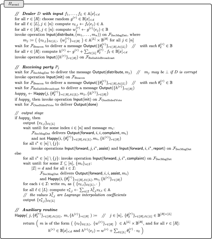
An AVSS protocol over $\mathbb {A}$

5.1.1 Additional Commentary

Analogously to what we did in the description of various broadcast and broadcast-like protocols in Sects. 3 and 4, we express the logic for the dealer as a separate process, even though the dealer is also one of the receiving parties. In particular, the dealer will receive an output from the random beacon, just like the receiving parties. We also define a subroutine $\textsf{Happy}$, which returns a Boolean value and may be called by any party.

The protocol starts when the dealer D is initiated with inputs $f_1, \ldots , f_L \in \mathbb {A}[x]_{< d}$. The dealer generates random “blinding” polynomials $g^{(r)} \in \mathbb {B}[x]_{< d}$ for $r\in [R]$. The dealer then computes shares of its input and “blinding” polynomials, that is, $v_{\ell ,j} {:}{=}f_\ell (e_j) \in \mathbb {A}$ for $\ell \in [L], j \in [n]$ and $w_j^{(r)} {:}{=}g^{(r)}(e_j) \in \mathbb {B}$ for $r\in [R],j\in [n]$. Next, the dealer sends each party $P_j$ its share of all of these polynomials as a message $m_j$ via the secure message distribution subprotocol. That is, $m_j = \big ( \ \{ v_{\ell ,j} \}_{\ell \in [L]}, \ \{ w_j^{(r)} \}_{r\in [R]} \ \big ) \in \mathbb {A}^{[L]} \times \mathbb {B}^{[R]}$—but if the dealer is corrupt, it may be that $m_j = \bot$.

Upon receiving $m_j$ via the secure message distribution subprotocol, party $P_j$ will initiate the random beacon subprotocol, and then wait for the output $\{ \theta _\ell ^{(r)} \}_{r\in [R],\ell \in [L]}$ of the random beacon. The random beacon output serves as a random “challenge”.

Given the random “challenge” from the beacon, the dealer D computes “response” polynomials $h^{(r)} {:}{=}g^{(r)} + \sum _{\ell \in [L]} \theta _\ell ^{(r)} \cdot f_\ell \in \mathbb {B}[x]_{< d}$ for $r \in [R]$, and then broadcasts these polynomials to all parties using the reliable broadcast subprotocol.

Upon receiving these “response” polynomials via the reliable broadcast subprotocol, each party $P_j$ checks the validity of the data it has received so far (this is done using the $\textsf{Happy}$ subroutine in the figure). Essentially, $P_j$ checks the identities $h^{(r)}(e_j) = w_j^{(r)} + \sum _{\ell \in [L]} \theta _\ell ^{(r)} \cdot v_{\ell ,j}$ for $r \in [R]$. If the dealer is honest, this check will certainly pass; however, if the dealer is corrupt, it may fail (and will certainly fail if $m_j=\bot$). If this check passes, $P_j$ sets $\textit{happy}_j$ to $\textsf{true}$, and we say $P_j$ is “happy”; otherwise, $P_j$ sets $\textit{happy}_j$ to $\textsf{false}$, and we say $P_j$ is “unhappy”.

Next, each party $P_j$ initiates the one-sided voting subprotocol if $\textit{happy}_j$ is $\textsf{true}$. If this subprotocol returns $\textsf {done}$, the parties enter the output stage.

In the output stage, a “happy” party $P_j$ may immediately output its shares $\{ v_{\ell ,j} \}_{\ell \in [L]}$, but waits around in case it receives a valid “complaint” from any “unhappy” party, to which it will respond by broadcasting an “assist” to all parties. Conversely, an “unhappy” party $P_j$ broadcasts a “complaint” against the dealer and then waits for sufficiently many valid “assists”, which will allow it to construct its correct shares.

A “complaint” is a message that is forwarded from a party via the secure message distribution subprotocol (with a $\textsf {complaint}$ tag) that serves as a proof that it is indeed “unhappy”—and that the dealer must be corrupt. An “assist” is also a message that is forwarded from a party via the secure message distribution subprotocol (with an $\textsf {assist}$ tag). These “complaints” and “assists” contain the original message received by a party in the secure message distribution subprotocol, and any other party may validate these messages (from the point of view of the “complaining” and “assisting” party). Of course, if the dealer is honest, there cannot be any “unhappy” parties —honest or corrupt. When an “unhappy” party receives d valid “assists”, this will allow it to compute its correct shares by polynomial interpolation. In the figure, for a subset $\mathcal {I} \subseteq [n]$ of size d, we denote by $\{\lambda ^{\mathcal {I}}_{i,j} \}_{i \in \mathcal {I},j \in [n]}$ the “Lagrange coefficients”, which are elements of $\mathbb {A}$ that satisfy

$$\begin{aligned} f(j) = \sum _{i \in \mathcal {I}} \lambda ^{\mathcal {I}}_{i,j} \cdot f(i) \end{aligned}$$

for any polynomial $f \in \mathbb {A}[x]_{< d}$, and which are efficiently computable. An “unhappy” party may use these Lagrange coefficients to compute its shares from the shares of its “happy” peers that provided valid “assists”.

Note that in the protocol, when a party broadcasts an “assist” it also broadcasts a “report” —this is a copy of the original “complaint” that triggered the “assist” broadcast, and it is sent using the forwarding mechanism (with a $\textsf {report}$ tag). The purpose of this is to ensure that if any honest party broadcasts a “complaint” or an “assist”, then all honest parties will eventually receive evidence that implicates the corrupt dealer. We do not specify here how parties process this evidence. For example, in the short term, once an honest party has identified a corrupt party, the honest party can safely ignore all messages from the corrupt party in future (or at least until some “proactive refresh” of the system occurs). When sufficiently many honest parties start ignoring a corrupt dealer, that dealer will no longer be able to trigger any more “complaints” or “assists”—at least, assuming we use protocol $\varPi _{\textrm{SecMsgDst}}$ for secure message distribution (or something similar), which guarantees that if sufficiently many honest parties ignore the dealer, no honest party will even receive any shares. In the longer term, the honest parties can vote to remove the corrupt party from the network. Also, such evidence of corrupt behavior could lead to legal or financial jeopardy for the corrupt party, and this in itself may be enough to discourage such behavior.

Without this extra step of broadcasting a “report”, an adversary could force the protocol off the “happy path”, causing the communication complexity to blow up, but without ever leading to a situation where all honest parties have obtained evidence that implicates the corrupt dealer. For example, a corrupt dealer could give bad shares to a corrupt party $P_j$, and then $P_j$ could “complain” to just a subset $\mathcal {S}$ of the honest parties. The members of $\mathcal {S}$ would all see the “complaints” and broadcast “assists”, but honest parties outside of $\mathcal {S}$ would never see any “complaints”, and the “assists” by themselves do not implicate the corrupt dealer.

If the dealer is honest, it is fairly easy to see that all honest parties will eventually output their shares of the dealer’s polynomials. Moreover, the “blinding” polynomials, together with the fact that no corrupt party can lodge a valid complaint against an honest dealer, will ensure that the adversary obtains no information about the dealer’s polynomials other than the shares belonging to corrupt parties.

Now suppose the dealer is corrupt. In this case, if any party enters the output stage, the one-sided voting protocol ensures that at least $n-2t \ge d$ honest parties are “happy” and that all honest parties eventually enter the output stage. In addition, these d “happy” honest parties will ensure that any “unhappy” honest parties eventually receive the “assists” that they need to obtain their shares. In the security proof, we will argue that with overwhelming probability, the shares of all the “happy” parties (honest or corrupt) must lie on polynomials of degree less than d, as required. For this argument to work, it is crucial that honest parties do not initiate the random beacon subprotocol before they receive their message from the secure message distribution subprotocol—this ensures that the “challenge” is not revealed before the dealer has committed to the entire message vector $(m_1, \ldots , m_n)$.

Although our protocol is a secure AVSS protocol, is has an interesting property. Namely, a corrupt dealer does not really commit to its input polynomials until after it obtains the “challenge” from the beacon and reveals its “response” polynomials. For example, let $n=3t+1$ and $d=t+1$. A corrupt dealer can give the honest parties completely uncorrelated random shares, and after receiving the “challenge”, it can choose a random set of $t+1$ honest parties, interpolate through just these parties’ shares to obtain corresponding input polynomials $f_1,\ldots ,f_L$, and then compute corresponding “response” polynomials. These $t+1$ honest parties together with the t corrupt parties can force all honest parties to output shares of $f_1,\ldots ,f_L$. Of course, in this example, the remaining t honest parties will “complain” against the dealer, proving that the dealer is corrupt.

5.2 Security Analysis

In order to analyze the failure probability of this generic protocol, we need the following definition.

Definition 5.1

(Inner product bound). With $\mathbb {A}$, $\mathbb {B}$, and $\varTheta \subseteq \mathbb {B}^L$ as above, we define

$$\begin{aligned} \chi (\mathbb {A},\mathbb {B},\varTheta ) \end{aligned}$$

to be the maximum, over all $b\in \mathbb {B}$ and nonzero $\varvec{a}\in \mathbb {A}^L$, of the probability that

$$\begin{aligned} b + \langle \varvec{a}, \varvec{\theta } \rangle = 0, \end{aligned}$$

where $\varvec{\theta }$ is chosen uniformly at random from $\varTheta$.

In a typical instantiation, one would choose $\mathcal {E}$ to be a maximum sized exceptional set in $\mathbb {B}$ so that we can apply Schwarz–Zippel (Lemma 2.1). In this setting, we have: if $\varTheta =\varTheta _{\textrm{pow}}^\mathcal {E}$, then $\chi (\mathbb {A},\mathbb {B},\varTheta ) \le L/|\mathcal {E} |$, and if $\varTheta =\varTheta _{\textrm{lin}}=\mathcal {E}^L$, then $\chi (\mathbb {A},\mathbb {B},\varTheta ) = 1/|\mathcal {E} |$. Choosing a larger ring $\mathbb {B}$ will allow one to increase the size of $\mathcal {E}$, however this comes at the expense of increasing the size of the elements which need to be transmitted.

Theorem 5.1

(Security of $\varPi _{\textrm{avss1}}$) Assume $2^n \cdot \chi (\mathbb {A},\mathbb {B},\varTheta )^R$ is negligible. Then we have:

• (i) $\varPi _{\textrm{avss1}}$ securely realizes $\mathcal {F}_{\textrm{avss}}$ in the $(\mathcal {F}_{\textrm{SecMsgDst}},\mathcal {F}_{\textrm{Beacon}},\mathcal {F}_{\textrm{ReliableBroadcast}},\mathcal {F}_{\textrm{OneSidedVote}})$-hybrid model.

• (ii) If $\varPi _{\textrm{avss1}}$ is instantiated with concrete protocols for $\mathcal {F}_{\textrm{SecMsgDst}}$, $\mathcal {F}_{\textrm{Beacon}}$, $\mathcal {F}_{\textrm{ReliableBroadcast}}$, and $\mathcal {F}_{\textrm{OneSidedVote}}$ that are secure (i.e., securely realize the corresponding functionality) and complete (i.e., satisfy the corresponding completeness property), then the resulting concrete protocol

  • (a) securely realizes $\mathcal {F}_{\textrm{avss}}$, and

  • (b) satisfies the AVSS completeness property.

Proof

We start with statement (i) of the theorem. To that end, we need to show that there is a simulator that interacts with $\mathcal {F}_{\textrm{avss}}$ in the ideal world such that no environment can effectively distinguish the ideal world from the hybrid world.

Without loss of generality, we may assume that in the hybrid world, the adversary is a “dummy” adversary that essentially acts as a “router” between the environment and the hybrid functionalities. In addition, in the ideal world, our simulator is actually in charge of implementing the hybrid functionalities. In particular, in the ideal world, any messages sent from (resp., to) the adversary to (resp., from) these hybrid functionalities are actually sent directly to (resp., from) our simulator—this including the inputs (resp., outputs) of corrupt parties.

If the dealer is honest, the proof reduces to showing that the values $\{ h^{(r)} \}_{r\in [R]}$ and $\{ w_j^{(r)} \}_{r\in [R]}$ for $j\in \mathcal {C}$ do not leak any extra information. This is a standard argument, based on the randomness supplied by the “blinding” polynomials $\{ g^{(r)} \}_{r\in [R]}$. In more detail, the ideal functionality $\mathcal {F}_{\textrm{avss}}$ gives the simulator the values $v_{\ell ,j}$ for $\ell \in [L]$ and $j\in \mathcal {C}$. For $r\in [R]$, the simulator then chooses $h^{(r)} \in \mathbb {B}[x]_{< d}$ at random, and then computes

$$\begin{aligned} w_j^{(r)} \leftarrow h^{(r)}(e_j) - \sum _{\ell \in [L]} \theta ^{(r)}_\ell \cdot v_{\ell ,j} \quad \text {(for } j \in \mathcal {C}). \end{aligned}$$

Note that the simulator can also generate the random beacon values $\theta ^{(r)}_\ell$ in advance of this computation.

The more interesting case is that when the dealer is corrupt. The crux of the proof in this case is showing that by the first point in time at which any honest party outputs its shares, the simulator can effectively extract corresponding polynomials $f_1,\ldots ,f_L\in F[x]_{< d}$. The proof is similar to the analysis in [22]. The main difference is that our protocol may terminate successfully if any subset of $n-2t$ honest parties is happy, and this subset may be determined after the random beacon is revealed. A simple way to deal with this is to apply the union bound to the collection of all subsets of parties, which is where the factor $2^n$ in the theorem statement comes from.

In more detail, consider the inputs $(m_1, \ldots , m_n)$ to $\mathcal {F}_{\textrm{SecMesDst}}$, where each $m_j$ is either $\bot$ or of the form

$$\begin{aligned} m_j = \big ( \ \{ v_{\ell ,j} \}_{\ell \in [L]}, \ \{ w_j^{(r)} \}_{r\in [R]} \ \Big ) , \end{aligned}$$

(1)

and which must be submitted to $\mathcal {F}_{\textrm{SecMsgDst}}$ and hence to our simulator, before the random beacon is revealed. (Here, we are essentially using the input extractability property of the secure message distribution protocol.) We will generally ignore indices j such that $m_j=\bot$.

Consider the later point in time at which some any party first enters the output stage. At this point in time, we can define $\mathcal {P}^*$ to be the set of indices $j \in [n]$ for which $P_j$ is happy, as determined by the input $m_j$, the random beacon value, and the “response” polynomials $h^{(r)}$. This set includes all parties, including honest parties $P_j$ that have not computed $\textit{happy}_j$, as well as corrupt parties. By the correctness property of the one-sided voting protocol, we have $|\mathcal {P}^* \cap \mathcal {H} | \ge n-2t \ge d$.

For each $\ell \in [L]$, the simulator extracts D’s input polynomial $f_\ell$ as the unique polynomial of degree less than $|\mathcal {P}^* |$ that interpolates through the points $\{ (e_j, v_{\ell ,j}) \}_{j\in \mathcal {P}^*}$. The simulation fails iff any of these polynomials has degree $\ge d$. Indeed, if any of these polynomials has degree $\ge d$, then the simulation obviously fails. Conversely, if all of these polynomials have degree $< d$, then one sees that the complaint mechanism works correctly: the honest parties hold enough good shares to reconstruct the polynomials by themselves (since $|\mathcal {P}^* \cap \mathcal {H} | \ge d$); moreover, the corrupt parties cannot contribute bad shares during this process (which is why we include corrupt parties in the definition of $\mathcal {P}^*$).

We want to bound the probability that the simulation fails. To this end, let us first make some definitions. Consider any fixed inputs $(m_1,\ldots ,m_n)$ to $\mathcal {F}_{\textrm{SecMsgDst}}$, where each $m_j = \bot$ or is of the form (1). Consider any set $\mathcal {P}\subseteq [n]$ with $n' {:}{=}|\mathcal {P} | \ge d$ and $m_j \ne \bot$ for all $j\in \mathcal {P}$. We say $\mathcal {P}$ is d -consistent if for each $\ell \in [L]$, the points $\{ (e_j,v_{\ell ,j})\}_{j \in \mathcal {P}}$ lie on a polynomial over $\mathbb {A}$ of degree less than d. Consider any fixed element $\{ \theta _\ell ^{(r)} \}_{r\in [R],\ell \in [L]}$ of the output space $\varOmega$ of the random beacon. We say $\mathcal {P}$ is d -consistent modulo $\{ \theta _\ell ^{(r)} \}_{r\in [R],\ell \in [L]}$ if for each $r \in [R]$, the points

$$\begin{aligned} \left\{ \ \left( \ e_j, \ w_j^{(r)} + \sum _{\ell \in [L]} \theta _\ell ^{(r)} \cdot v_{\ell ,j} \ \right) \ \right\} _{j \in \mathcal {P}} \end{aligned}$$

lie on a polynomial over $\mathbb {B}$ of degree less than d.

Claim If $\mathcal {P}$ is not d-consistent, then the probability that it is d-consistent modulo a randomly chosen element of $\varOmega$ is at most $\chi (\mathbb {A},\mathbb {B},\varTheta )^R$.

To prove the claim, we consider the $(n', d)$-Reed-Solomon code over $\mathbb {A}$ with respect to the evaluation coordinates $\{ e_j \}_{j\in \mathcal {P}}$, and the corresponding check matrix $C \in \mathbb {A}^{n'\times (n'-d)}$. We also consider the corresponding “extended” $(n',d)$-Reed-Solomon code over the extension ring $\mathbb {B}$, which has the same check matrix C as our original code (since the evaluation coordinates lie in $\mathbb {A}$).

Now suppose $\mathcal {P}$ is not d-consistent. For $\ell \in [L]$, define the vector

$$\begin{aligned} \varvec{v}_\ell {:}{=}\{ v_{\ell ,j}\}_{j \in \mathcal {P}} \in \mathbb {A}^{n'}. \end{aligned}$$

The assumption that $\mathcal {P}$ is not d-consistent means that for some $\ell ^*\in [L]$, the vector $\varvec{v}_{\ell ^*}$ is not a codeword, which means $\varvec{v}_{\ell ^*}\cdot C \ne 0$. So if we define the matrix $Q \in \mathbb {A}^{L\times n'}$ whose $\ell$-th row is $\varvec{v}_\ell$ for $\ell \in [L]$, then $Q\cdot C \in \mathbb {A}^{L\times (n'-d)}$ is nonzero matrix.

Now suppose $\mathcal {P}$ is d-consistent modulo $\{ \theta _\ell ^{(r)} \}_{r\in [R],\ell \in [L]}$. For each $r\in [R]$, define

$$\begin{aligned} \varvec{w}^{(r)} {:}{=}\{ w_j^{(r)} \}_{j\in \mathcal {P}} \in \mathbb {B}^{n'} \quad \text {and}\quad \varvec{\theta }^{(r)} {:}{=}(\theta _1^{(r)}, \ldots , \theta _L^{(r)}) \in \varTheta \end{aligned}$$

so that

$$\begin{aligned} \varvec{w}^{(r)} + \varvec{\theta }^{(r)}\cdot Q \end{aligned}$$

lies in the extended Reed-Solomon code, which implies

$$\begin{aligned} \varvec{w}^{(r)}\cdot C + \varvec{\theta }^{(r)}\cdot Q\cdot C = 0 . \end{aligned}$$

(2)

Since $Q\cdot C$ is a nonzero matrix, we can choose one nonzero column of $Q\cdot C$, and (2) implies that for some fixed $b\in \mathbb {B}$ and fixed, nonzero $\varvec{a} \in \mathbb {A}^L$, we have

$$\begin{aligned} b + \langle \varvec{a}, \varvec{\theta }^{(r)} \rangle = 0 . \end{aligned}$$

(3)

So for each $r\in [R]$, if we choose $\varvec{\theta }^{(r)} \in \varTheta$ at random, equation (3) holds with probability at most $\chi (\mathbb {A},\mathbb {B},\varTheta )$, and repeating this R times gives the desired probability and proves the claim.

We now return to the task of bounding the probability that the simulation fails. If the simulation fails, this implies that $\mathcal {P}^*$ is not d-consistent yet is d-consistent modulo the output of the random beacon. Now, even though the inputs to $\mathcal {F}_{\textrm{SecMsgDst}}$ are chosen before the random beacon is revealed, the subset $\mathcal {P}^*$ is chosen by the adversary after the random beacon is revealed. Nevertheless, for the simulation to fail, the following event must occur: the adversary submits inputs to $\mathcal {F}_{\textrm{SecMsgDst}}$ such that there exists a subset $\mathcal {P}\subseteq [n]$ of the required form that is not d-consistent but ends up being d-consistent modulo the output of the random beacon. As there are at most $2^n$ choices for $\mathcal {P}$, by the union bound, the probability that the simulation fails is therefore at most $2^n \cdot \chi (\mathbb {A},\mathbb {B},\varTheta )^R$.

That proves statement (i) of the theorem. Statement (ii)(a) is a direct consequence of statement (i) and the UC composition theorem. Statement (ii)(b) easily follows from the security and completeness properties of the concrete subprotocols, and the logic of $\varPi _{\textrm{avss1}}$, along the lines discussed in Sect. 5.1.1. $\square$

Note that we obtain a somewhat better failure bound when we use $\varTheta = \varTheta _{\textrm{lin}}^\mathcal {E}$. However, in this instantiation, our random beacon has to output very long vectors $(\theta _1,\ldots ,\theta _L) \in \mathcal {E}^L$. As discussed in Sect. 3.1.2, this could be avoided by using a random beacon that outputs a short seed that is then stretched using a cryptographic pseudorandom generator G. This implementation will indeed be secure if we model G as a random oracle. However, we cannot justify the security of this implementation if we simply assume that G is a pseudorandom generator. As discussed in Sect. 3.1.2, to do this, it would suffice that the failure event in Theorem 5.1 can be efficiently detected as a function of the output of G and data that are available to the adversary prior to revealing the beacon. Unfortunately, this event is a union over an exponentially large set of events, and so is not efficiently detectable.

Note that the factor $2^n$ in the failure bound in Theorem 5.1 does not arise in the analysis of the corresponding protocol in [22]. For modest sized n, this should be acceptable, using a larger extension $\mathbb {B}$, or larger value of R, as necessary. Of course, using a larger $\mathbb {B}$ or R can impact communication complexity. This is discussed in detail below in Sect. 5.3. However, in some important applications, $\mathbb {A}$ is a field of size $\approx 2^{256}$, and so for $n \le 128$, we already get nearly 128-bit security with $\mathbb {B}=\mathbb {A}$ and $R=1$.

An example. Here is a simple example that shows why an exponential factor in the failure probability in Theorem 5.1 seems hard to avoid. This example gives a specific, efficient adversary and specific protocol parameters such that the adversary breaks the security of the protocol with probability $2^{\varOmega (n)} \cdot \chi (\mathbb {A},\mathbb {B},\varTheta )^R$.

Let $n = 3t+1$, $d=t+1$, $L=1$, $R=1$, $\mathbb {B}=\mathbb {A}$, and $\varTheta = \varTheta _{\textrm{pow}}$. The corrupt dealer starts the protocol by distributing shares of $g {:}{=}x^{t+2} + x^{t+1}$ and $f {:}{=}x^{t+2}$ (which play the roles of $g^{(1)}$ and $f_1$, respectively, in the protocol). Now consider any set $\mathcal {P}\subseteq [n]$ of size $t+2$, and define

$$\begin{aligned} g^{(\mathcal {P})} {:}{=}g \bmod \prod _{j\in \mathcal {P}}(x-e_j) \end{aligned}$$

and

$$\begin{aligned} f^{(\mathcal {P})} {:}{=}f \bmod \prod _{j\in \mathcal {P}}(x-e_j). \end{aligned}$$

Then we have

$$\begin{aligned} g^{(\mathcal {P})} = (1+T^{(\mathcal {P})}) \cdot x^{t+1} + \text {lower order terms} \end{aligned}$$

and

$$\begin{aligned} f^{(\mathcal {P})} = T^{(\mathcal {P})} \cdot x^{t+1} + \text {lower order terms}, \end{aligned}$$

where

$$\begin{aligned} T^{(\mathcal {P})} {:}{=}-\sum _{j\in \mathcal {P}} e_i. \end{aligned}$$

For a given challenge $\theta$, the adversary will break the protocol if it can find a subset $\mathcal {P}\subseteq \mathcal {H}$ of size $t+2$ such that

$$\begin{aligned} (1+T^{(\mathcal {P})}) + \theta \cdot T^{(\mathcal {P})} = 0, \end{aligned}$$

or in other words

$$\begin{aligned} T^{(\mathcal {P})} = -1/(1+\theta ). \end{aligned}$$

Indeed, in this case, the adversary can compute a response polynomial that makes the parties in $\mathcal {P}$ happy, even though their shares do not lie on a polynomial of degree at most t. Moreover, the t corrupt parties, together with the parties in $\mathcal {P}$, can force the one-sided voting protocol to succeed, so all honest parties enter the output stage. To obtain an efficient attack that succeeds with probability at least $2^{\varOmega (n)}/|\mathbb {B} |$, it suffices that the map $\mathcal {P}\mapsto T^{(\mathcal {P})}$ is (nearly) one-to-one and easy to invert. For example, if $|\mathbb {A} | > 2^n$ and the evaluation coordinates are $1,2,\dots , 2^{n-1}$, then this is the case.

5.3 Communication Complexity

We now consider the communication complexity of $\varPi _{\textrm{avss1}}$. Here, the communication complexity of a protocol is defined to be the sum of the length of all messages sent by honest parties (to either honest or corrupt parties) over the point-to-point channels.

We make a distinction between the “happy path” and the “unhappy path”. To enter the “unhappy path”, a corrupt party must provably misbehave. In our protocol, this corresponds to the situation where a party complains against a corrupt dealer. If this happens, all honest parties will learn of this and can take action: in the short term, the honest parties can safely ignore this party, and in the longer term, the corrupt party can be removed from the network. Also, such provable misbehavior could lead to legal or financial jeopardy for the corrupt party, and this in itself may be enough to discourage such behavior. Note that the “happy path” includes corrupt behavior, including collusion among the corrupt parties, as well as behavior that is clearly corrupt as observed by an individual honest party, but that cannot be used as reliable evidence to convince other honest parties or an external authority of corrupt behavior.

For these reasons, we believe it makes sense to make a distinction between the complexity of the protocol on the “happy path” versus the “unhappy path”.

We also make a couple of simplifying assumptions. Namely, we assume that $\mathbb {B}=\mathbb {A}$ and that $\varTheta = \varTheta _{\textrm{lin}}^\mathcal {E}$, where $\mathcal {E}$ is an exceptional set of maximal size. In this case, the failure bound in Theorem 5.1 becomes $2^n /|\mathcal {E} |^R$. We will want to set R so that this bound is negligible. This is discussed below.

5.3.1 The Happy Path

Each message $m_j$ input into the $\mathcal {F}_{\textrm{SecMsgDst}}$ has size

$$\begin{aligned} O\left( (L+R) \cdot \log |\mathbb {A} | \right) . \end{aligned}$$

Our protocol $\varPi _{\textrm{SecMsgDst}}$ for secure message distribution from Sect. 4 has communication complexity $O(|\textbf{m} | + \lambda \cdot n^2\cdot \log n )$, and so its contribution to the total communication complexity is

$$\begin{aligned} O \left( n \cdot (L+R) \cdot \log |\mathbb {A} | + \lambda \cdot n^2\cdot \log n \right) . \end{aligned}$$

The message input to $\mathcal {F}_{\textrm{ReliableBroadcast}}$ is of size $O(n \cdot R \cdot \log |\mathbb {A} |)$. Using protocol $\varPi _{\textrm{CompactBroadcast}}$ from Sect. 3.2.2, this contributes

$$\begin{aligned} O\left( n^2 \cdot R \cdot \log |\mathbb {A} | + \lambda \cdot n^2\cdot \log n \right) \end{aligned}$$

to the overall communication complexity. We may implement $\mathcal {F}_{\textrm{OneSidedVote}}$ as in Sect. 3.2.5, which contributes $O(n^2)$ to the communication complexity. We shall ignore for now the communication complexity of the random beacon. Thus, the total communication complexity, ignoring the random beacon, is

$$\begin{aligned} O \left( n \cdot (L+n R) \cdot \log |\mathbb {A} | + \lambda \cdot n^2\cdot \log n \right) . \end{aligned}$$

(4)

If we want $\sigma$ bits of security, we should select R as

$$\begin{aligned} R = \Big \lceil \frac{\sigma +n}{\log _2 |\mathcal {E} |} \Big \rceil . \end{aligned}$$

(5)

With this setting of R, our communication complexity bound (4) becomes

$$\begin{aligned} O \left( n \cdot L\cdot \log |\mathbb {A} | + n^2 \cdot (\sigma +n) \cdot \frac{\log |\mathbb {A} | }{\log |\mathcal {E} |} + \lambda \cdot n^2\cdot \log n \right) . \end{aligned}$$

(6)

5.3.2 Finite Field Case

Suppose $\mathbb {A}$ is a field extension of degree $\delta$ over the finite field $\mathbb {S}=\mathbb {F}_q$. In this case, $\mathcal {E}=\mathbb {A}$ and $|\mathbb {A} | = |\mathbb {S} |^\delta$; therefore, (6) simplifies to

$$\begin{aligned} O \left( n \cdot L\cdot \delta \cdot \log |\mathbb {S} | + n^3 + n^2 \cdot \sigma + \lambda \cdot n^2 \cdot \log n \right) , \end{aligned}$$

and if $\max \{n,\sigma \} \le \lambda$, this simplifies even further to

$$\begin{aligned} O \left( n \cdot L\cdot \delta \cdot \log |\mathbb {S} | + \lambda \cdot n^2 \cdot \log n \right) . \end{aligned}$$

While we have ignored the communication complexity of the random beacon, we may assume it is bounded by a polynomial in n and $\lambda$ (which, in practice, is typically $O(n^2 \lambda )$). Therefore, for sufficiently large L (polynomial in n, $\sigma$, and $\lambda$) the amortized communication complexity per sharing is

$$\begin{aligned} O(n \cdot \delta \cdot \log |\mathbb {S} |). \end{aligned}$$

Suppose that our AVSS protocol is used in an application where the secrets lie in the field $\mathbb {S}=\mathbb {F}_q$, where $q \le n$. In this case, as discussed in Sect. 2.4, we will have to run our protocol over a field $\mathbb {A}$ of degree $\delta$ over $\mathbb {S}$, where $\delta = \lceil \log _q (n+1) \rceil$. In this case, the amortized communication complexity per sharing is

$$\begin{aligned} O(n \cdot \log _q n \cdot \log |\mathbb {S} |), \end{aligned}$$

which is

$$\begin{aligned} O(n \cdot \log n). \end{aligned}$$

5.3.3 Galois Ring Case

Suppose $\mathbb {A}$ is a Galois ring of degree $\delta$ over the ring $\mathbb {S}={\mathbb {Z}}/(p^k)$. In this case, $|\mathbb {A} | = |\mathbb {S} |^\delta = p^{k \cdot \delta }$ but $|\mathcal {E} | = p^\delta$, and (6) simplifies to

$$\begin{aligned} O \left( n \cdot L\cdot \delta \cdot \log |\mathbb {S} | + n^2 \cdot (\sigma +n) \cdot k + \lambda \cdot n^2\cdot \log n \right) . \end{aligned}$$

Therefore, for sufficiently large L (polynomial in n, $\sigma$, $\lambda$, and k) the amortized communication complexity per sharing is

$$\begin{aligned} O(n \cdot \delta \cdot \log |\mathbb {S} |). \end{aligned}$$

Suppose that our AVSS protocol is used in an application where the secrets lie in the ring $\mathbb {S}={\mathbb {Z}}/(p^k)$, where $p \le n$. In this case, as discussed in Sect. 2.4, we will have to run our protocol over a Galois ring $\mathbb {A}$ of degree $\delta$ over $\mathbb {S}$, where $\delta = \lceil \log _p (n+1) \rceil$. In this case, the amortized communication complexity per sharing is

$$\begin{aligned} O(n \cdot \log _p n \cdot \log |\mathbb {S} |), \end{aligned}$$

which is

$$\begin{aligned} O( n \cdot \log n \cdot k). \end{aligned}$$

5.3.4 The Unhappy Path

For the “unhappy path”, the communication complexity of the secure message distribution protocol may blow up by a factor of n. So in this case, the bound (4) becomes

$$\begin{aligned} O \left( n^2 \cdot (L+R) \cdot \log |\mathbb {A} | + \lambda \cdot n^3\cdot \log n \right) , \end{aligned}$$

and choosing R as in (5), the bound (6) becomes

$$\begin{aligned} O \left( n^2 \cdot L\cdot \log |\mathbb {A} | + n^2 \cdot (\sigma +n) \cdot \frac{\log |\mathbb {A} | }{\log |\mathcal {E} |} + \lambda \cdot n^3\cdot \log n \right) . \end{aligned}$$

Thus, all of our estimates above for amortized communication complexity per sharing get blown up by a factor of n.

5.3.5 Message Complexity

The message complexity of $\varPi _{\textrm{avss1}}$ on both the “happy path” and the “unhappy path”, not including the random beacon, is $O(n^2)$. Here, the message complexity of a protocol is defined to be the total number of messages sent by honest parties (to either honest or corrupt parties) over the point-to-point channels. In practice, the message complexity of the random beacon is typically also $O(n^2)$.

6 Restricting the Secrets to a Subring

We assume here that a secret is encoded, as usual, as the constant term of a polynomial. As discussed in Sect. 2.4, our AVSS protocol may be used in an application where the secrets lie in a ring $\mathbb {S}$ that does not contain the appropriate evaluation coordinates, and we are forced to run our AVSS protocol in an extension ring $\mathbb {A}$ that does contain such coordinates. In this section, we give an AVSS protocol that enforces the restriction that the shared secret in fact lies in $\mathbb {S}$. Our protocol works when $\mathbb {S}$ and $\mathbb {A}$ are Galois rings, and does secret sharing over a related ring $\mathbb {A}'$. Our AVSS protocol that enforces this restriction makes use of a subprotocol for secret sharing over $\mathbb {A}'$. Our technique for ensuring inputs lie in $\mathbb {S}$ makes use of the checking technique of extending the p-adic precision one works with, which was first introduced in [15].

6.1 Auxiliary Rings

We begin by describing the relationship between the various rings involved. Let $G(z) \in {\mathbb {Z}}[z]$ be a monic polynomial of degree $\epsilon \ge 1$. Let $F(y, z)\in {\mathbb {Z}}[y,z]$ be a bivariate polynomial of the form

$$\begin{aligned} F(y,z) = F_0(z) + F_1(z) \cdot y + \cdots + F_{\delta -1}(z) \cdot y^{\delta -1} + y^\delta , \end{aligned}$$

where $\delta \ge 1$. For each $m \ge 1$, define the rings

$$\begin{aligned} \mathbb {S}^{(m)} {:}{=}{\mathbb {Z}}[z]/(p^m, G(z)) \quad \text {and}\quad \mathbb {A}^{(m)} {:}{=}{\mathbb {Z}}[y,z]/(p^m,G(z),F(y,z)). \end{aligned}$$

We naturally view ${\mathbb {Z}}/(p^m) \subseteq \mathbb {S}^{(m)} \subseteq \mathbb {A}^{(m)}$ as a tower of ring extensions, where $\mathbb {S}^{(m)}$ has degree $\epsilon$ over ${\mathbb {Z}}/(p^m)$ and $\mathbb {A}^{(m)}$ has degree $\delta$ over $\mathbb {S}^{(m)}$. Indeed, every element of $\mathbb {A}^{(m)}$ can be expressed uniquely as the image of a polynomial in ${\mathbb {Z}}[y,z]$ of the form $A_0(z) + A_1(z) \cdot y + \cdots + A_{\delta -1}(z) \cdot y^{\delta -1}$, where for $i = 0, \ldots , \delta -1$, we have $\deg A_i < \epsilon$, and each coefficient of $A_i$ lies in the interval $[0,p^m)$. The ring $\mathbb {S}^{(m)}$ corresponds to the subset of such polynomials of degree at most 0 in y. The ring ${\mathbb {Z}}/(p^m)$ corresponds to the subset of such polynomials of degree at most 0 in y and z.

We shall require that $\mathbb {S}^{(1)}$ and $\mathbb {A}^{(1)}$ are fields. This requirement ensures that $\mathbb {S}^{(m)}$ and $\mathbb {A}^{(m)}$ are Galois rings. Note that for $m' \ge m$, there is a natural map from $\mathbb {A}^{(m')}$ to $\mathbb {A}^{(m)}$, and the restriction of this map to $\mathbb {S}^{(m')}$ is the natural map from $\mathbb {S}^{(m')}$ to $\mathbb {S}^{(m)}$. The units in $\mathbb {A}^{(m)}$ are the elements whose images in $\mathbb {A}^{(1)}$ are nonzero (this follows from Hensel lifting).

We fix a sequence polynomials $E_1, \ldots , E_n \in {\mathbb {Z}}[y,z]$ whose images in $\mathbb {A}^{(1)}$ form an exceptional sequence. Note that for every $m \ge 1$, the images of these polynomials in $\mathbb {A}^{(m)}$ also form an exceptional sequence in $\mathbb {A}^{(m)}$.

Now fix an integer $k \ge 1$ and define

$$\begin{aligned} \mathbb {S}{:}{=}\mathbb {S}^{(k)} \quad \text {and}\quad \mathbb {A}{:}{=}\mathbb {A}^{(k)}. \end{aligned}$$

Let $e_1, \ldots , e_n \in \mathbb {A}$ be the images of $E_1,\ldots ,E_n$ in $\mathbb {A}$. Our ring of secrets will be $\mathbb {S}$. Our goal is to design a secret sharing protocol that can be used to share of a secret in $\mathbb {S}$, where the evaluation coordinates are $e_1, \ldots , e_n$, and so the shares lie in $\mathbb {A}$ even though the secret lies in $\mathbb {S}$. Such a protocol should provide all the usual guarantees of any secret sharing protocol, but should also enforce the restriction that the shared secret is in $\mathbb {S}$, even if the dealer is corrupt.

To do this, we will actually perform a secret sharing over another ring. Fix an integer $k' \ge k$ and define

$$\begin{aligned} \mathbb {S}' {:}{=}\mathbb {S}^{(k')} \quad \text {and}\quad \mathbb {A}' {:}{=}\mathbb {A}^{(k')}. \end{aligned}$$

Let $e_1', \ldots , e_n' \in \mathbb {A}'$ be the images of $E_1,\ldots ,E_n$ in $\mathbb {A}'$. Let $\phi$ be the natural map from $\mathbb {A}'$ to $\mathbb {A}$. Observe that $\mathbb {S}'$ is a subring of $\phi ^{-1}(\mathbb {S})$. The idea is that we will do the following steps:

• 1. Perform a sharing of a secret in $\mathbb {S}'$ with shares in $\mathbb {A}'$, with respect to the evaluation coordinates $e'_1, \ldots , e'_n$.

• 2. Perform a probabilistic check that ensures that the secret lies in $\phi ^{-1}(\mathbb {S})$ with high probability.

After this, each party can locally apply $\phi$ to its share to obtain a sharing of a secret in $\mathbb {S}$ with shares in $\mathbb {A}$, with respect to the evaluation coordinates $e_1,\ldots ,e_n$.

On the one hand, if the dealer is honest, in order to protect the privacy of the dealer’s secret, it is essential that their secret $s'$ lies in $\mathbb {S}'$. Of course, an honest dealer should really be starting out with a secret in $s\in \mathbb {S}$ and then choose $s'\in \mathbb {S}'$ as some (arbitrary) preimage of s under $\phi$. On the other hand, if the dealer is corrupt, the protocol does not enforce the constraint that the dealer’s secret lies in $\mathbb {S}'$, but only that it lies in $\phi ^{-1}(\mathbb {S})$. In either case, after each party locally applies $\phi$ to its share, we end up with a sharing of a secret in $\mathbb {S}$.

6.2 Two Special Cases

We briefly sketch how the above general setting includes two important special cases.

$\mathbb {S}$ is a non-prime finite field:

This corresponds to the setting where $k=1$ and $\epsilon > 1$. In this case, $\mathbb {S}={\mathbb {Z}}[z]/(p,G(z))$ is a finite field of cardinality $q = p^{\epsilon }$, and $\mathbb {A}={\mathbb {Z}}[y,z]/(p,G(z),F(y,z))$ is an extension field of degree over $\delta$ over $\mathbb {F}_q$ (and so has $q^\delta = p^{\epsilon \cdot \delta }$ elements). We also have corresponding rings $\mathbb {S}'={\mathbb {Z}}[z]/(p^{k'},G(z))$ and $\mathbb {A}'=Z[y,z]/(p^{k'},G(z),F(y,z))$. Note that even though $\mathbb {S}$ and $\mathbb {A}$ are fields, $\mathbb {S}'$ and $\mathbb {A}'$ will not be (assuming $k'>1$).

$\mathbb {S}$ is of the form ${\mathbb {Z}}/(p^k)$::

This corresponds to setting $G(z) {:}{=}z$, and using a polynomial of the form $F(y) \in {\mathbb {Z}}[y]$ in the role of F(y, z). Then $\mathbb {S}={\mathbb {Z}}/(p^k)$ and $\mathbb {A}={\mathbb {Z}}[y]/(p^k,F(y))$. We also have corresponding rings $\mathbb {S}'={\mathbb {Z}}/(p^{k'})$ and $\mathbb {A}'={\mathbb {Z}}[y]/(p^{k'},F(y))$.

6.3 The Protocol

The basic idea is this. The dealer has polynomials $f_1,\ldots ,f_L \in \mathbb {A}'[x]_{< d}$, where for each $\ell \in [L]$, the corresponding secret is the constant term $f_\ell (0)$, which lies in $\mathbb {S}'$. The dealer chooses a random “blinding” polynomial $g \in \mathbb {A}'[x]_{< d}$ also with $g(0) \in \mathbb {S}'$, and then runs an AVSS protocol on the polynomials $f_1, \ldots , f_L, g$. After this, a random beacon is used to generate a random “challenge”

$$\begin{aligned} \varvec{\gamma } {:}{=}(\gamma _1, \ldots , \gamma _L) \in ({\mathbb {Z}}/(p^{k'}))^L. \end{aligned}$$

The dealer then computes the “response” polynomial

$$\begin{aligned} h \leftarrow g + \sum _{\ell \in [L]} \gamma _\ell \cdot f_\ell , \end{aligned}$$

(7)

which is also a polynomial in $\mathbb {A}'[x]_{< d}$ with $h(0) \in \mathbb {S}'$, and reliably broadcasts h. After receiving the polynomial h and verifying that it is of the correct form (i.e., of the right degree and with constant term in $\mathbb {S}'$), each party $P_j$ verifies that h is locally correct based on its shares by checking that (7) holds at the evaluation coordinate $e'_j$. The parties then run a trivial voting protocol that will ensure that they only output their shares if at least $n-2t \ge d$ parties have successfully performed this local check. This ensures that (7) holds. We then argue that if $f_{\ell ^*}(0) \notin \phi ^{-1}(\mathbb {S})$ for some $\ell ^*\in [L]$, then the probability that $h(0) \in \mathbb {S}'$ for randomly chosen $\varvec{\gamma }$ is at most $p^{k-k'-1}$. This implies that except with probability $p^{k-k'-1}$, we can be sure that the secret $f_\ell (0)$ lies in $\phi ^{-1}(\mathbb {S})$ all $\ell \in [L]$.

Our protocol, which we call $\varPi _{\textrm{ravss1}}$, is presented in Fig. 12. It makes use of a repetition parameter R, so that the above probabilistic check is actually performed R times. It makes use of an $(n,d,L+R)$-AVSS subprotocol over $\mathbb {A}'$ with respect to $(e'_1, \ldots , e'_n)$. In the description of $\varPi _{\textrm{ravss1}}$, we invoke this as an ideal functionality $\mathcal {F}_{\textrm{avss}}$. Protocol $\varPi _{\textrm{ravss1}}$ also makes use of

• A random beacon whose output space is defined to be

  $$\begin{aligned} \Big \{ \ \big \{ \gamma _\ell ^{(r)} \big \}_{\ell \in [L],r\in [R]} \, \ \gamma _\ell ^{(r)} \in {\mathbb {Z}}/(p^{k'}) \ \Big \}, \end{aligned}$$

  which is invoked as an ideal functionality $\mathcal {F}_{\textrm{Beacon}}$;

• A reliable broadcast subprotocol, which is invoked as an ideal functionality $\mathcal {F}_{\textrm{ReliableBroadcast}}$.

As we shall argue below, when the protocol produces an output, the shared secrets must lie in $\phi ^{-1}(\mathbb {S})$ (with high probability). As mentioned above, each party can then locally apply $\phi$ to its shares to obtain sharings of secrets in $\mathbb {S}$.

Fig. 12

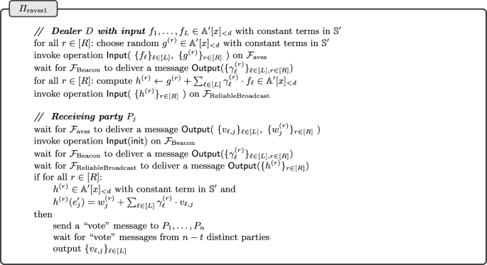
AVSS protocol for a dealer to provably enter values in $\phi ^{-1}(\mathbb {S})$

6.4 Security Analysis

To analyze the security of $\varPi _{\textrm{ravss1}}$ (Fig. 13), we begin with the following simple lemma.

Lemma 6.1

Let p be a prime and let s be a positive integer. Let $a_1, \ldots , a_L$ be integers, not all zero mod $p^s$. Let r be the largest positive integer such that $p^r$ divides $a_\ell$ for $\ell \in [L]$, so that $r < s$. Let b be an arbitrary integer. Let N be the number of integers $x_1, \ldots , x_L$ in the range $[0,p^s)$ that satisfy

$$\begin{aligned} a_1 \cdot x_1 + \cdots a_L \cdot x_L + b \equiv 0 \pmod {p^s} . \end{aligned}$$

(8)

Then $N/p^{L \cdot s} \le p^{r-s}$.

Proof

Without loss of generality, assume that $p^r \mid a_1$ but $p^{r+1} \not \mid a_1$. We may assume $p^r \mid b$, as otherwise (8) has no solutions. In this case, (8) holds iff

$$\begin{aligned} (a_1/p^r) \cdot x_1 + \cdots (a_L/p^r) \cdot x_L + (b/p^r) \equiv 0 \pmod {p^{s-r}}. \end{aligned}$$

Moreover, since $a_1/p^r$ is not divisible by p, for every choice of $x_2, \ldots , x_L$, there is a unique choice of $x_1$ mod $p^{s-r}$, and so $p^r$ choices for $x_1$ in the interval $[0,p^s)$. The lemma follows. $\square$

This lemma says that if $x_1, \ldots , x_L$ are randomly chosen from the interval $[0,p^s)$, then the probability that (8) holds is at most $p^{r-s}$.

Fig. 13

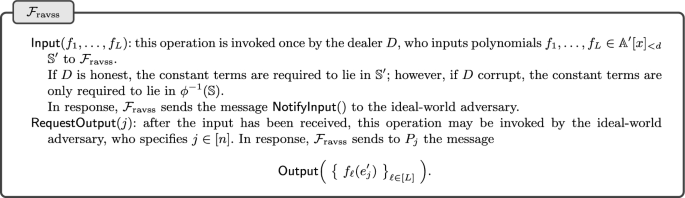
The restricted AVSS ideal functionality (parameterized by n, d, L, R, D, p, k, $k'$, F, G, $(E_1,\ldots ,E_n)$, which define $\mathbb {S}$, $\mathbb {A}$, $\mathbb {S}'$, $\mathbb {A}'$, $\phi$, and $e'_1, \ldots , e'_n$)

Theorem 6.1

(Security of $\varPi _{\textrm{ravss1}}$) Assume $p^{(k-k'-1) \cdot R}$ is negligible. Then we have:

• (i) $\varPi _{\textrm{ravss1}}$ securely realizes $\mathcal {F}_{\textrm{ravss}}$ in the $(\mathcal {F}_{\textrm{avss}},\mathcal {F}_{\textrm{Beacon}},\mathcal {F}_{\textrm{ReliableBroadcast}})$-hybrid model.

• (ii) If $\varPi _{\textrm{ravss1}}$ is instantiated with concrete protocols for $\mathcal {F}_{\textrm{avss}}$, $\mathcal {F}_{\textrm{Beacon}}$, and $\mathcal {F}_{\textrm{ReliableBroadcast}}$ that are secure (i.e., securely realize the corresponding functionality) and complete (i.e., satisfy the corresponding completeness property), then the resulting concrete protocol

  • (a) securely realizes $\mathcal {F}_{\textrm{ravss}}$, and

  • (b) satisfies the AVSS completeness property.

Proof

We start with statement (i) of the theorem. To that end, we need to show that there is a simulator that interacts with $\mathcal {F}_{\textrm{ravss}}$ in the ideal world such that no environment can effectively distinguish the ideal world from the hybrid world.

If the dealer is honest, the proof reduces to showing that the values $h^{(r)}$ and $w_j^{(r)}$ for $j\in \mathcal {C}$ and $r\in [R]$ do not leak any extra information. This is a standard argument, based on the “random padding” supplied by the polynomials $g^{(r)}$. In more detail, the ideal functionality $\mathcal {F}_{\textrm{ravss}}$ gives the simulator the values $v_{\ell ,j}$ for $\ell \in [L]$ and $j\in \mathcal {C}$. For each $r\in [r]$, the simulator then chooses $h^{(r)} \in \mathbb {A}'[x]_{< d}$ with constant term in $\mathbb {S}'$ at random and then computes

$$\begin{aligned} w_j^{(r)} \leftarrow h^{(r)}(e'_j) - \sum _{\ell \in [L]} \gamma _\ell ^{(r)} \cdot v_{\ell ,j} \quad \text {(for }j \in \mathcal {C}). \end{aligned}$$

Note that the simulator can also generate the random beacon values $\gamma _\ell ^{(r)}$ in advance of this computation.

Now consider case is that when the dealer is corrupt. The dealer must submit polynomials $\{ f_\ell \}_{\ell \in [L]}$ and $\{ g^{(r)} \}_{r\in [R]}$ of degree less than d to $\mathcal {F}_{\textrm{avss}}$ before the random beacon values $\gamma _\ell ^{(r)}$ are revealed. Let $s_\ell$ denote the constant term of $f_\ell$ for $\ell \in [L]$ and let $s^{(r)}$ denote the constant term of $g^{(r)}$ for $r\in [R]$. If and when an honest party produces an output, the simulator needs to submit $\{ f_\ell \}_{\ell \in [L]}$ to the ideal functionality $\mathcal {F}_{\textrm{ravss}}$, and so the simulation will fail if some $s_\ell$ is not in $\phi ^{-1}(\mathbb {S})$. To bound the probability that this simulation fails, suppose that $s_{\ell ^*} \notin \phi ^{-1}(\mathbb {S})$ for some particular $\ell ^*\in [L]$. To finish the proof of the theorem, it will suffice to show that for randomly chosen $\{ \gamma _\ell ^{(r)} \}_{\ell \in [L],r\in [R]}$ the probability that any honest party ever produces an output is at most $p^{(k-k'-1) \cdot R}$.

Suppose that some honest party produces an output. The honest party that produced an output received $n-t$ “vote” messages, which means that at least $n-2t \ge d$ honest parties performed their local checks and these checks passed. This implies that each $h^{(r)}$ has the correct form (is of degree less than d with constant term in $\mathbb {S}'$), and that

$$\begin{aligned} h^{(r)} = g^{(r)} + \sum _{\ell \in [L]} \gamma _\ell ^{(r)} \cdot f_\ell \quad \text {(for all }r\in [R]). \end{aligned}$$

(9)

This implies that

$$\begin{aligned} s^{(r)} + \sum _{\ell \in [L]} \gamma _\ell ^{(r)} \cdot s_\ell \in \mathbb {S}' \quad \text {(for all }r\in [R]). \end{aligned}$$

(10)

So it suffices to show that (10) holds with probability at most $p^{(k-k'-1) \cdot R}$.

For $\ell \in [L]$, we can express $s_\ell$ uniquely as the image in $\mathbb {A}'$ of a polynomial in ${\mathbb {Z}}[y,z]$ of the form

$$\begin{aligned} \sum _{i=0}^{\delta -1} \sum _{j=0}^{\epsilon -1} a_{i,j,\ell } \cdot y^i \cdot z^j, \end{aligned}$$

where each $a_{i,j,\ell }$ is an integer in the range $[0,p^{k'})$. The assumption that $s_{\ell ^*} \notin \phi ^{-1}(\mathbb {S})$ means that for some $i^* \ge 1$ and $j^* \ge 0$, we have $a_{i^*,j^*,\ell ^*} \not \equiv 0 \pmod {p^k}$. For $r\in [R]$, we can similar express $s^{(r)}$ uniquely as the image in $\mathbb {A}'$ of a polynomial in ${\mathbb {Z}}[y,z]$ of the form

$$\begin{aligned} \sum _{i=0}^{\delta -1} \sum _{j=0}^{\epsilon -1} b_{i,j} \cdot y^i \cdot z^j, \end{aligned}$$

For $\ell \in [L]$ and $r\in [R]$, we can view each $\gamma _\ell ^{(r)}$ as the image in ${\mathbb {Z}}/(p^{k'})$ of a randomly chosen integer $x_\ell ^{(r)}$ in the range $[0,p^{k'})$. But then by (10), we must have

$$\begin{aligned} b_{i^*,j^*} + \sum _{\ell \in [L]} a_{i^*,j^*,\ell } \cdot x_\ell ^{(r)} \equiv 0 \pmod {p^{k'}} \quad \text {(for all } r\in [R]). \end{aligned}$$

(11)

But by Lemma 6.1, the congruence (11) holds with probability at most $p^{(k-k'-1) \cdot R}$.

That proves statement (i) of the theorem. Statement (ii)(a) is a direct consequence of statement (i) and the UC composition theorem. Statement (ii)(b) follows fairly easily from the security and completeness properties of the concrete subprotocols, and the logic of $\varPi _{\textrm{ravss1}}$. The argument in the case where the dealer is honest is entirely straightforward. The argument in the case where the dealer is corrupt hinges on the following observation. In the hybrid version of $\varPi _{\textrm{ravvs1}}$, as we argued above, if one honest party produces an output, then at least $n-2t \ge d$ honest parties must have performed their local checks and these checks passed, and this implies that each $h^{(r)}$ has the correct form and (9) must hold. This means that when any honest party performs its local check, that check will pass and it will broadcast a “vote” message. Since this property always holds in the hybrid version of $\varPi _{\textrm{ravvs1}}$, it must hold with overwhelming probability in the concrete version of $\varPi _{\textrm{ravvs1}}$ as well. Therefore, in the concrete version of $\varPi _{\textrm{ravvs1}}$, if one honest party produces an output, then with overwhelming probability, all parties will eventually do so. $\square$

After the proof of Theorem 5.1, we remarked that in some instantiations, we cannot justify the use of a random beacon that generates a short seed that is then stretched using a pseudorandom generator (as discussed in Sect. 3.1.2). That limitation does not apply here. Indeed, as discussed in Sect. 3.1.2, to do this, it suffices that the failure event in Theorem 6.1 can be efficiently detected as a function of the output of G and data that are available to the adversary prior to revealing the beacon. The reader can verify that this is the case.

Note that the completeness argument at the end of the above proof would have been simpler if instead of the trivial one-round voting protocol, we used the one-sided voting protocol $\varPi _{\textrm{OneSidedVote}}$, which has two rounds. Note also that if we instantiate $\mathcal {F}_{\textrm{avss}}$ with our protocol $\varPi _{\textrm{avss1}}$, which already performs a one-sided vote, the resulting protocol could be optimized by combining these two voting steps into just a single one-sided vote.

6.5 Communication Complexity

We calculate the communication complexity of this protocol. We assume the AVSS protocol in Sect. 5 protocol is used for sharing over $\mathbb {A}'$ and we consider the amortized complexity on the “happy path”—but we could use any AVSS protocol that achieves linear amortized communication complexity of the “happy path”. In this setting, the communication complexity (amortized, “happy path”) is

$$\begin{aligned} O(n \cdot \log |\mathbb {A}' |). \end{aligned}$$

The settings of the parameters R and $k'$ affect both the communication complexity and the failure bound.

6.5.1 Setting $k'{:}{=}k$

At one extreme, we could set $k'{:}{=}k$. In this case, to achieve $\sigma$ bits of security, we need to set the repetition parameter $R {:}{=}\lceil \sigma \cdot \log _p 2 \rceil$. The main advantage of this parameter setting is that $\mathbb {A}'=\mathbb {A}$, and the amortized communication complexity remains the same as in Sect. 5.3. The main disadvantage of this setting is that the amortized computational complexity blows up by a factor of R.

6.5.2 Setting $R{:}{=}1$

At another extreme, we could set $R{:}{=}1$. In this case, to achieve $\sigma$ bits of security, we need to set $k' {:}{=}k - 1 + \lceil \sigma \cdot \log _p 2 \rceil$. Assuming $\mathbb {S}$ has degree $\epsilon$ over ${\mathbb {Z}}/(p^k)$ and $\mathbb {A}$ has degree $\delta$ over $\mathbb {S}$ the complexity (amortized, “happy path”) is

$$\begin{aligned} O(n \cdot \delta \cdot (\log |\mathbb {S} | + \epsilon \cdot \sigma )). \end{aligned}$$

Finite Field Case. Suppose $\mathbb {A}$ is a field extension of degree $\delta$ over the finite field $\mathbb {S}=\mathbb {F}_q$, where $q = p^\epsilon$, $\delta = O(\log _q n)$, and $k=1$. Then the communication complexity (amortized, “happy path”) is

$$\begin{aligned} O(n \cdot \log _q n \cdot (\log |\mathbb {S} | + \epsilon \cdot \sigma ) ), \end{aligned}$$

which is

$$\begin{aligned} O( n \cdot \log n \cdot (1 + \sigma /\log p) ). \end{aligned}$$

Galois Ring Case. Suppose $\mathbb {S}={\mathbb {Z}}/(p^k)$ and $\mathbb {A}$ is of degree $\delta =O(\log _p n)$ over $\mathbb {S}$, so $\epsilon =1$. Then the communication complexity (amortized, “happy path”) is

$$\begin{aligned} O(n \cdot \log _p n \cdot (\log |\mathbb {S} | + \sigma ) ), \end{aligned}$$

which is

$$\begin{aligned} O( n \cdot \log n \cdot (k + \sigma /\log p) ). \end{aligned}$$

As a special case, suppose $p=2$ and k is large enough so that $2^{-k}$ is negligible. Then by setting $k' {:}{=}2k$, we obtain $k+1$ bits of security, while both the amortized communication and computational complexity increase by just a small constant factor over the basic AVSS protocol.

7 Random Oracle Implementations

In this section, we present a variant of our new AVSS protocol $\varPi _{\textrm{avss1}}$ (from Sect. 5), as well a variant of the AVSS protocol $\varPi _{\textrm{ravss1}}$ (from Sect. 6, which restricts the dealer’s secrets). These variants do not need a random beacon; rather, they require that we model a hash function as a random oracle in the security analysis. Besides eliminating the need for a random beacon subprotocol, these variants require significantly fewer rounds of communication.

7.1 A Random Oracle Version of $\varPi _{\textrm{avss1}}$

At a very high level, protocol $\varPi _{\textrm{avss1}}$ in Sect. 5 is based on the classical commit–challenge–response paradigm, which we can view as an interactive game between the dealer and a challenger:

• 1. The dealer sends a vector of messages $\textbf{m}=(m_1,\ldots ,m_n)$ to the challenger.

• 2. The challenger generates a random challenge $\omega \in \varOmega$ and sends this to the dealer.

• 3. The dealer responds with a message $m'$.

In $\varPi _{\textrm{avss1}}$:

• the messages $m_1, \ldots , m_n$ encode the shares of the dealer’s input polynomials, which are distributed using a secure message distribution subprotocol,

• the challenge is generated using a distributed random beacon subprotocol, and

• the response $m'$ encodes the dealer’s “response” polynomials, which are broadcast using a reliable broadcast subprotocol.

The main idea is to replace the distributed random beacon subprotocol by a hash function that is modeled as a random oracle. This way, the dealer can interact exclusively with the random oracle to generate a 3-move “conversation”, consisting of $(\textbf{m},\omega ,m')$, and then disseminate this conversation to all parties in a way that satisfies the privacy, correctness, and completeness properties of secure message distribution and reliable broadcast, and that includes support for the “forwarding mechanism” of secure message distribution.

7.1.1 A Subprotocol for Disseminating 3-Move Conversations

We show how to carry out this idea by sketching a protocol we call $\varPi _{\textrm{Dst3move}}$.

The dealer will first build a Merkle tree as shown in Fig. 14. It uses the same Merkle tree structure, rooted at r, used in our secure message distribution protocol $\varPi _{\textrm{SecMsgDst}}$ in Sect. 4.3 to encrypt and encode $\textbf{m}=(m_1,\ldots ,m_n)$, and the same Merkle tree structure, rooted at $r'$, used in the compact reliable broadcast protocol $\varPi _{\textrm{CompactBroadcast}}$ in Sect. 3.2.2 to encode $m'$. In addition, the dealer creates a new Merkle tree with root $\hat{r}'$ whose children are r and $r'$. We assume that the hash that outputs the root r also outputs the challenge $\omega$.

We assume that all hash functions queries are properly domain separated, meaning that we always include an input to the hash that identifies the individual instance of the protocol, including the identity of the dealer. We also assume that for a given protocol instance, different uses of the hash function are further domain separated. In particular, we assume that the hashes used to

• derive $(r,\omega )$,

• derive $\hat{r}'$,

• compute H in $\varPi _{\textrm{SecMsgDst}}$, and

• create all other nodes of Merkle trees,

are domain separated from each other. This domain separation greatly simplifies the analysis in the random oracle model.

Fig. 14

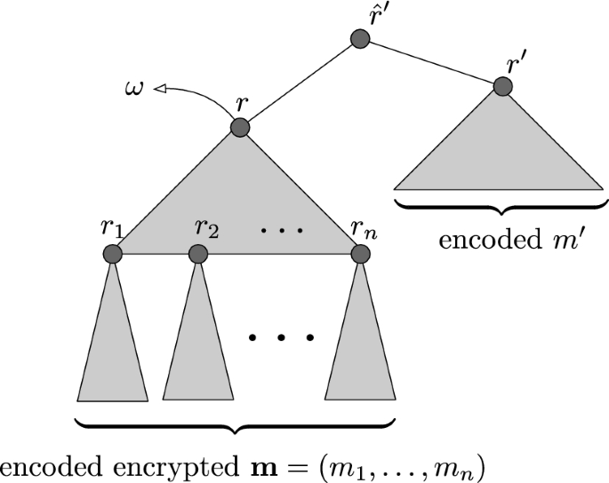
Merkle tree structure for a 3-move conversation

Next, the dealer initiates a subprotocol to distribute each $m_j$ to each $P_j$ as in $\varPi _{\textrm{SecMsgDst}}$ and broadcast $m'$ to all parties as in $\varPi _{\textrm{CompactBroadcast}}$. This subprotocol has the same send-echo-vote structure as in each of these protocols. However, in this subprotocol, all echoing/voting is done on the “global” root $\hat{r}'$ of the entire structure, so that just one round of send-echo-vote suffices to distribute the $m_j$’s and to broadcast $m'$. In particular, the message sent by the dealer to a party $P_j$ will include $\hat{r}'$, r, and $r'$, as well as

• $r_i$ and the jth validated path in the Merkle tree rooted at $r_i$ for all $i \in [n]$, and

• the jth validated path in the Merkle tree rooted at $r'$.

In response, each party sends echo messages, where each echo message contains the root $\hat{r}'$, along with

• the validated path starting at r it would normally send in $\varPi _{\textrm{SecMsgDst}}$, and

• the validated path starting at $r'$ it would normally send in $\varPi _{\textrm{CompactBroadcast}}$.

The forwarding mechanism is implemented in precisely the same way as in $\varPi _{\textrm{SecMsgDst}}$.

Note that in this construction, the dealer explicitly includes the hash values r and $\hat{r}'$ in the send messages, and the receiver verifies that these are consistent with $r_1, \ldots , r_n$ and $r'$, rather than just computing r and $\hat{r}'$. This simplifies the analysis in the random oracle model, as we can assume that when the dealer is corrupt, it must have already invoked the random oracle to obtain r and $\hat{r}'$ explicitly before sending to an honest party (as otherwise that party will almost surely ignore the message).

In order to analyze the security of $\varPi _{\textrm{Dst3move}}$, we rely on the fact that for a corrupt dealer, we have the following extractability property: by observing the random oracle queries of the adversary, a simulator can effectively determine the committed input $\textbf{m}=(m_1, \ldots , m_n)$ before the random challenge $\omega$ is generated—note that some of the $m_j$’s may be $\bot$ if the adversary has not made the necessary random oracle queries. We also rely on the fact that for an honest dealer, we have the following equivocability property: a simulator is free to program the random oracle (the one that outputs the random challenge) so that it outputs a given random challenge $\omega$. To justify this, we have to ensure that the input to this hash has high entropy and so that adversary is unlikely to have queried the random oracle previously at this point; however, this will be the case, since in the protocol, the input to this hash query (the one that outputs $(r,\omega )$) is ultimately derived from the outputs of the H hash function in $\varPi _{\textrm{SecMsgDst}}$, and these outputs are essentially random.

We also observe that an adversary can carry out a “grinding” attack. Indeed, an adversary can effectively:

• try many different message vectors, where for each such message vector $\textbf{m}$, it builds a Merkle tree and derives the corresponding challenge $\omega$, creating a partial conversation $(\textbf{m},\omega )$,

• pick one such partial conversation $(\textbf{m},\omega )$ that it likes,

• extend $(\textbf{m},\omega )$ with a message $m'$ of its choice to obtain a full conversation $(\textbf{m},\omega ,m')$, and finally

• disseminate the full conversation $(\textbf{m},\omega ,m')$ to all parties.

We can characterize the security of protocol $\varPi _{\textrm{Dst3move}}$ in terms of an ideal functionality $\mathcal {F}_{\textrm{Dst3move}}$. To this functionality, the dealer submits a message vector $\textbf{m}=(m_1,\ldots ,m_n)$ and obtains a random challenge $\omega$, creating the partial conversation $(\textbf{m},\omega )$. After this, the dealer submits a message $m'$, creating the full conversation $(\textbf{m},\omega ,m')$. This full conversation is then disseminated to all parties following the semantics of $\mathcal {F}_{\textrm{SecMsgDst}}$ and $\mathcal {F}_{\textrm{ReliableBroadcast}}$—in particular, for an honest dealer, the only information leaked to the ideal-world adversary is the challenge $\omega$, the final message $m'$, and (implicitly) the messages $m_j$ belonging to corrupt parties $P_j$.

To model the above “grinding” attack, the functionality also allows a corrupt dealer to repeatedly submit a message vector $\textbf{m}$, obtaining a challenge $\omega$ and creating the partial conversation $(\textbf{m},\omega )$. We call one such operation a grind on $\mathcal {F}_{\textrm{Dst5move}}$. At some point, the corrupt dealer may choose a partial extended conversation $(\textbf{m},\omega )$ and submit a message $m'$, creating the full conversation $(\textbf{m},\omega ,m')$, which is then disseminated to all parties following the semantics of $\mathcal {F}_{\textrm{SecMsgDst}}$ and $\mathcal {F}_{\textrm{ReliableBroadcast}}$.

We leave it to the reader to verify that $\varPi _{\textrm{Dst3move}}$ securely realizes the ideal functionality $\mathcal {F}_{\textrm{Dst3move}}$. Moreover, in the security reduction, the number of grinds on $\mathcal {F}_{\textrm{Dst3move}}$ made by the simulator is bounded by the number of random oracle queries made by the real-world adversary.

We also leave it to the reader to verify that $\varPi _{\textrm{Dst3move}}$ enjoys completeness properties analogous to those of $\varPi _{\textrm{SecMsgDst}}$ and $\varPi _{\textrm{ReliableBroadcast}}$.

7.1.2 An AVSS Protocol

To build an AVSS protocol using $\varPi _{\textrm{Dst3move}}$, we use $\varPi _{\textrm{Dst3move}}$ as a drop-in replacement in $\varPi _{\textrm{avss1}}$ for $\mathcal {F}_{\textrm{SecMsgDst}}$, $\mathcal {F}_{\textrm{Beacon}}$, and $\mathcal {F}_{\textrm{ReliableBroadcast}}$. The only remaining steps of $\varPi _{\textrm{avss1}}$ are local computations and $\mathcal {F}_{\textrm{OneSidedVote}}$. The result is a protocol we denote by $\varPi _{\textrm{avss2}}$.

We leave it to the reader to verify the following. Notation is as in Theorem 5.1.

Theorem 7.1

(Security of $\varPi _{\textrm{avss2}}$) Assume $Q \cdot 2^n \cdot \chi (\mathbb {A},\mathbb {B},\varTheta )^R$ is negligible, where Q is the number of grinds on $\mathcal {F}_{\textrm{Dst3move}}$. Then we have:

• (i) $\varPi _{\textrm{avss2}}$ securely realizes $\mathcal {F}_{\textrm{avss}}$ in the $(\mathcal {F}_{\textrm{Dst3move}},\mathcal {F}_{\textrm{OneSidedVote}})$-hybrid model.

• (ii) If $\varPi _{\textrm{avss2}}$ is instantiated with concrete protocols for $\mathcal {F}_{\textrm{Dst3move}}$ and $\mathcal {F}_{\textrm{OneSidedVote}}$, that are secure (i.e., securely realize the corresponding functionality) and complete (i.e., satisfy the corresponding completeness property), then the resulting concrete protocol

  • (a) securely realizes $\mathcal {F}_{\textrm{avss}}$, and

  • (b) satisfies the AVSS completeness property.

The communication complexity of $\varPi _{\textrm{avss2}}$ is essentially the same as that of $\varPi _{\textrm{avss1}}$. However, in terms of rounds of communication, $\varPi _{\textrm{avss2}}$ is significantly better. Indeed (on the happy path), if we instantiate $\varPi _{\textrm{avss2}}$ with $\varPi _{\textrm{Dst3Move}}$ and $\varPi _{\textrm{OneSidedVote}}$, we see that it needs 3 rounds for $\varPi _{\textrm{Dst3move}}$ and 2 rounds for $\varPi _{\textrm{OneSidedVote}}$, for a total of just 5 rounds. In contrast, if we instantiate $\varPi _{\textrm{avss1}}$ with $\varPi _{\textrm{SecMsgDst}}$, $\varPi _{\textrm{CompactBroadcast}}$, $\varPi _{\textrm{OneSidedVote}}$, and any 1-round protocol that realizes $\mathcal {F}_{\textrm{Beacon}}$, we that it needs 3 rounds for $\varPi _{\textrm{SecMsgDst}}$, 1 round for the beacon, 3 rounds for $\varPi _{\textrm{CompactBroadcast}}$, and 2 rounds for $\varPi _{\textrm{OneSidedVote}}$, for a total of 9 rounds.

We speculate that $\varPi _{\textrm{avss2}}$ can be further optimized by folding the one-sided voting subprotocol into $\varPi _{\textrm{Dst3Move}}$ in such a way that the total number of rounds is 4 rather than 5; however, we have not carried out the associated full design and analysis.

We also speculate that $\varPi _{\textrm{avss2}}$ can be implemented in such a way that it is secure against adaptive corruptions in the random oracle model. To achieve this, it should be sufficient to use an equivocable symmetric encryption scheme as discussed in Sect. 4.3. However, we have not carried out the associated full design and analysis.

7.2 A Random Oracle Version of $\varPi _{\textrm{ravss1}}$

Let us assume that we instantiate $\mathcal {F}_{\textrm{avss}}$ in protocol $\varPi _{\textrm{ravss1}}$ with $\varPi _{\textrm{avss1}}$. The resulting protocol then has the following structure of a 5-move interactive game between the dealer and a challenger:

• 1. The dealer sends a vector of messages $\textbf{m}=(m_1,\ldots ,m_n)$ to the challenger.

• 2. The challenger generates a random challenge $\omega \in \varOmega$ and sends this to the dealer.

• 3. The dealer sends a message $m'$ to the challenger.

• 4. The challenger generates a random challenge $\omega '\in \varOmega '$ and sends this to the dealer.

• 5. The dealer responds with a message $m''$.

Here, moves 1–3 are as in $\varPi _{\textrm{avss1}}$, while moves 4 and 5 correspond to the challenge–response phase of $\varPi _{\textrm{ravss1}}$. One might hope to reduce these 5 moves to just 3 moves, but we do not see a way to do that. Indeed, as remarked in Sect. 5.1.1, a corrupt dealer only commits to its input polynomials after move 3, and in order for the security proof of Theorem 6.1 to go through, we cannot afford to reveal the challenge $\omega '$ until that occurs.

As above in Sect. 7.1, the main idea is to replace the distributed random beacon subprotocols by hash functions that are modeled as random oracles—the dealer can interact exclusively with the random oracle to generate a 5-move “conversation”, consisting of $(\textbf{m},\omega ,m',\omega '',m'')$, and then disseminate this conversation to all parties. We sketch here a protocol $\varPi _{\textrm{Dst5move}}$ that does exactly this.

The dealer will first build a Merkle tree as shown in Fig. 15. The structure is the same as in Fig. 14, except that we have added a Merkle subtree, rooted at $r''$, with the same structure as the compact reliable broadcast protocol $\varPi _{\textrm{CompactBroadcast}}$ in Sect. 3.2.2 to encode $m''$, and a “global” root $\hat{r}''$ with $\hat{r}'$ and $r''$ as children. We assume that the hash that outputs the root $\hat{r}'$ also outputs the challenge $\omega '$. We also assume all hashes are properly domain separated as discussed above Sect. 7.1, and in particular, the hashes used to derive $(r,\omega )$, $(\hat{r}',\omega ')$, and $\hat{r}''$ are all domain separated from each other as well as from other use cases.

Fig. 15

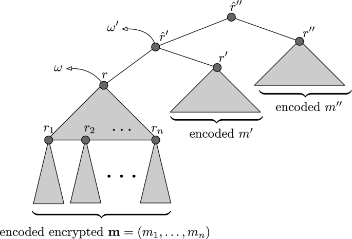
Merkle tree structure for 5-move conversation

Next, the dealer initiates a subprotocol to distribute each $m_j$ to each $P_j$ as in $\varPi _{\textrm{SecMsgDst}}$, broadcast $m'$ to all parties as in $\varPi _{\textrm{CompactBroadcast}}$, and broadcast $m''$ to all parties as in $\varPi _{\textrm{CompactBroadcast}}$. As above in Sect. 7.1, this subprotocol has a send-echo-vote structure, and all echoing/voting is done on the “global” root $\hat{r}''$, so that just one round of send-echo-vote suffices to distribute the $m_j$’s and to broadcast $m',m''$. Analogously to what we did in Sect. 7.1, the dealer explicitly includes the hash values r, $\hat{r}'$, and $\hat{r}''$ in the send messages

We can characterize the security of protocol $\varPi _{\textrm{Dst5move}}$ in terms of an ideal functionality $\mathcal {F}_{\textrm{Dst5move}}$. To this functionality, the dealer submits a message vector $\textbf{m}=(m_1,\ldots ,m_n)$ and obtains a random challenge $\omega$, creating the partial conversation $(\textbf{m},\omega )$. After this, the dealer submits a message $m'$ and obtains a random challenge $\omega '$, creating the extended conversation $(\textbf{m},\omega ,m',\omega ')$. Finally, the dealer submits $m''$, creating the full conversation $(\textbf{m},\omega ,m',\omega ',m'')$, which is then disseminated to all parties following the semantics of $\mathcal {F}_{\textrm{SecMsgDst}}$ and $\mathcal {F}_{\textrm{ReliableBroadcast}}$.

To model a “grinding” attack, the functionality also allows a corrupt dealer to repeatedly submit a message vector $\textbf{m}$, obtaining a challenge $\omega$ and creating the partial conversation $(\textbf{m},\omega )$. The corrupt dealer may also repeatedly choose any such partial $(\textbf{m},\omega )$ conversation, submit a message $m'$, obtaining a challenge $\omega '$ and creating the extended conversation $(\textbf{m},\omega ,m',\omega ')$. We call either one of the above operations a grind on $\mathcal {F}_{\textrm{Dst5move}}$. At some point, the corrupt dealer may choose an extended conversation $(\textbf{m},\omega ,m',\omega ')$ and submit a message $m''$, creating the full conversation $(\textbf{m},\omega ,m',\omega ',m'')$, which is then disseminated to all parties following the semantics of $\mathcal {F}_{\textrm{SecMsgDst}}$ and $\mathcal {F}_{\textrm{ReliableBroadcast}}$.

We leave it to the reader to verify that $\varPi _{\textrm{Dst5move}}$ securely realizes the ideal functionality $\mathcal {F}_{\textrm{Dst5move}}$. Moreover, in the security reduction, the number of grinds on $\mathcal {F}_{\textrm{Dst5move}}$ made by the simulator is bounded by the number of random oracle queries made by the real-world adversary.

We also leave it to the reader to verify that $\varPi _{\textrm{Dst5move}}$ enjoys completeness properties analogous to those of $\varPi _{\textrm{SecMsgDst}}$ and $\varPi _{\textrm{ReliableBroadcast}}$.

We now sketch how to build a variant of $\varPi _{\textrm{ravss1}}$ protocol using $\varPi _{\textrm{Dst5move}}$. First, recall that we are assuming here that we instantiate $\mathcal {F}_{\textrm{avss}}$ in $\varPi _{\textrm{ravss1}}$ with $\varPi _{\textrm{avss1}}$. Next, observe that both $\varPi _{\textrm{ravss1}}$ and the subprotocol $\varPi _{\textrm{avss1}}$ use a voting step to express whether they are happy with the information they have received. As noted after Theorem 6.1, we can safely combine these two voting steps into a single one-sided vote. That is, each party $P_j$ receives $(m_j,\omega ,m',\omega ',m'')$, and checks if $(m_j,\omega ,m')$ is valid according to $\varPi _{\textrm{avss1}}$, and checks if $(\bar{m}_j,\omega ',m'')$ is valid according to $\varPi _{\textrm{ravss1}}$ (here, $\bar{m}_j$ is the same as $m_j$, but with shares of blinding polynomials specific to $\varPi _{\textrm{avss1}}$ filtered out). A single one-sided vote (i.e., $\varPi _{\textrm{OneSidedVote}}$) can be used to attest that both of these checks pass. We then use $\varPi _{\textrm{Dst5move}}$ to replace all steps other than local computations and this one-sided voting step. The result is a protocol we denote by $\varPi _{\textrm{ravss2}}$.

We leave it to the reader to verify the following. Notation is as in Theorems 5.1 and 7.1, but where R is the repetition parameter for $\varPi _{\textrm{avss1}}$ and $R'$ is the repetition parameter for $\varPi _{\textrm{ravss1}}$:

Theorem 7.2

(Security of $\varPi _{\textrm{ravss2}}$) Assume $Q \cdot \big ( 2^n \cdot \chi (\mathbb {A},\mathbb {B},\varTheta )^R + p^{(k-k'-1) \cdot R'} \big )$ is negligible, where Q is the number of grinds on $\mathcal {F}_{\textrm{Dst5move}}$ Then we have:

• (i) $\varPi _{\textrm{ravss2}}$ securely realizes $\mathcal {F}_{\textrm{ravss}}$ in the $(\mathcal {F}_{\textrm{Dst5move}},\mathcal {F}_{\textrm{OneSidedVote}})$-hybrid model.

• (ii) If $\varPi _{\textrm{ravss2}}$ is instantiated with concrete protocols for $\mathcal {F}_{\textrm{Dst5move}}$ and $\mathcal {F}_{\textrm{OneSidedVote}}$, that are secure (i.e., securely realize the corresponding functionality) and complete (i.e., satisfy the corresponding completeness property), then the resulting concrete protocol

  • (a) securely realizes $\mathcal {F}_{\textrm{ravss}}$, and

  • (b) satisfies the AVSS completeness property.

The communication complexity of $\varPi _{\textrm{ravss2}}$ is essentially the same as that of $\varPi _{\textrm{ravss1}}$. However, in terms of rounds of communication, $\varPi _{\textrm{ravss2}}$ is significantly better. Indeed (on the happy path), it needs just 5 rounds of communication (the same as $\varPi _{\textrm{avss1}})$. In contrast, if we instantiate $\varPi _{\textrm{ravss1}}$ with $\varPi _{\textrm{SecMsgDst}}$, $\varPi _{\textrm{CompactBroadcast}}$, $\varPi _{\textrm{OneSidedVote}}$, and any 1-round protocol that realizes $\mathcal {F}_{\textrm{Beacon}}$, we that it needs 3 rounds for $\varPi _{\textrm{SecMsgDst}}$ in $\varPi _{\textrm{avss1}}$, 1 round for the beacon in $\varPi _{\textrm{avss1}}$, 3 rounds for the $\varPi _{\textrm{CompactBroadcast}}$ in $\varPi _{\textrm{avss1}}$, 2 rounds for $\varPi _{\textrm{OneSidedVote}}$ in $\varPi _{\textrm{avss1}}$, 1 round for the beacon in $\varPi _{\textrm{ravss1}}$, 3 rounds for the $\varPi _{\textrm{CompactBroadcast}}$ in $\varPi _{\textrm{ravss1}}$, 1 round for the simplified one-sided vote in $\varPi _{\textrm{ravss1}}$, for a total of 14 rounds.

Just as for $\varPi _{\textrm{avss2}}$, we speculate that $\varPi _{\textrm{ravss2}}$ can be further optimized so that the total number of rounds is 4 rather than 5. In addition, we also speculate that $\varPi _{\textrm{ravss2}}$ can be implemented in such a way that it is secure against adaptive corruptions in the random oracle model.

References

M. Abspoel, R. Cramer, I. Damgård, D. Escudero, C. Yuan, Efficient information-theoretic secure multiparty computation over \(\mathbb{Z}/p^k\mathbb{Z}\) via galois rings. In D. Hofheinz and A. Rosen, editors, TCC 2019: 17th Theory of Cryptography Conference, Part I, volume 11891 of Lecture Notes in Computer Science, Nuremberg, Germany, Dec. 1–5, (Springer, Heidelberg, Germany, 2019), pp. 471–501
M. Abspoel, R. Cramer, I. Damgård, D. Escudero, M. Rambaud, C. Xing, C. Yuan, Asymptotically good multiplicative LSSS over Galois rings and applications to MPC over \(\mathbb{Z}/p^k\mathbb{Z}\). In S. Moriai and H. Wang, editors, Advances in Cryptology – ASIACRYPT 2020, Part III, volume 12493 of Lecture Notes in Computer Science, Daejeon, South Korea, Dec. 7–11, (Springer, Heidelberg, Germany, 2020), pp. 151–180
I. Abraham, P. Jovanovic, M. Maller, S. Meiklejohn, G. Stern, Bingo: Adaptivity and asynchrony in verifiable secret sharing and distributed key generation. In H. Handschuh and A. Lysyanskaya, editors, Advances in Cryptology – CRYPTO 2023, Part I, volume 14081 of Lecture Notes in Computer Science, Santa Barbara, CA, USA, Aug. 20–24, (Springer, Heidelberg, Germany, 2023), pp. 39–70,
A. Bandarupalli, A. Bhat, S. Bagchi, A. Kate, M. Reiter, HashRand: Efficient asynchronous random beacon without threshold cryptographic setup. Cryptology ePrint Archive, Paper 2023/1755, 2023. https://eprint.iacr.org/2023/1755.
M. Ben-Or, R. Canetti, O. Goldreich, Asynchronous secure computation. In 25th Annual ACM Symposium on Theory of Computing, San Diego, CA, USA, May 16–18, (ACM Press, 1993), pp. 52–61
M. Bellare, J. A. Garay, T. Rabin, Batch verification with applications to cryptography and checking. In C. L. Lucchesi and A. V. Moura, editors, LATIN 1998: Theoretical Informatics, 3rd Latin American Symposium, volume 1380 of Lecture Notes in Computer Science, Campinas, Brazil, Apr. 20–24, 1998. (Springer, Heidelberg, Germany, 1998), pp. 170–191
D. Boneh, B. Lynn, H. Shacham, Short signatures from the Weil pairing. In C. Boyd, editor, Advances in Cryptology – ASIACRYPT 2001, volume 2248 of Lecture Notes in Computer Science, Gold Coast, Australia, Dec. 9–13, (Springer, Heidelberg, Germany, 2001), pp. 514–532
D. Bogdanov, S. Laur, J. Willemson, Sharemind: A framework for fast privacy-preserving computations. In S. Jajodia and J. López, editors, ESORICS 2008: 13th European Symposium on Research in Computer Security, volume 5283 of Lecture Notes in Computer Science, Málaga, Spain, Oct. 6–8, (Springer, Heidelberg, Germany, 2008), pp. 192–206
A. Boldyreva, Threshold signatures, multisignatures and blind signatures based on the gap-Diffie-Hellman-group signature scheme. In Y. Desmedt, editor, PKC 2003: 6th International Workshop on Theory and Practice in Public Key Cryptography, volume 2567 of Lecture Notes in Computer Science, Miami, FL, USA, Jan. 6–8, (Springer, Heidelberg, Germany, 2003), pp. 31–46
M. Bellare, P. Rogaway, Random oracles are practical: A paradigm for designing efficient protocols. In D. E. Denning, R. Pyle, R. Ganesan, R. S. Sandhu, and V. Ashby, editors, ACM CCS 93: 1st Conference on Computer and Communications Security, Fairfax, Virginia, USA, Nov. 3–5, (ACM Press, 1993), pp. 62–73
G. Bracha, Asynchronous Byzantine agreement protocols. Inf. Comput., 75(2), 130–143 (1987)
Z. Beerliová-Trubíniová, M. Hirt, Efficient multi-party computation with dispute control. In S. Halevi and T. Rabin, editors, TCC 2006: 3rd Theory of Cryptography Conference, volume 3876 of Lecture Notes in Computer Science, New York, NY, USA, Mar. 4–7, (Springer, Heidelberg, Germany, 2006), pp. 305–328
Z. Beerliová-Trubíniová, M. Hirt, Perfectly-secure MPC with linear communication complexity. In R. Canetti, editor, TCC 2008: 5th Theory of Cryptography Conference, volume 4948 of Lecture Notes in Computer Science, San Francisco, CA, USA, Mar. 19–21, (Springer, Heidelberg, Germany, 2008), pp. 213–230
R. Canetti, Universally composable security: A new paradigm for cryptographic protocols. Cryptology ePrint Archive, Report 2000/067, 2000. https://eprint.iacr.org/2000/067
R. Cramer, I. Damgård, D. Escudero, P. Scholl, C. Xing, SPD \(\mathbb{Z}_{2^k}\): Efficient MPC mod \(2^k\) for dishonest majority. In H. Shacham and A. Boldyreva, editors, Advances in Cryptology – CRYPTO 2018, Part II, volume 10992 of Lecture Notes in Computer Science, Santa Barbara, CA, USA, Aug. 19–23, (Springer, Heidelberg, Germany, 2018), pp. 769–798
J. H. Cheon, D. Kim, K. Lee. MHz2k: MPC from HE over \(\mathbb{Z}_{2^k}\) with new packing, simpler reshare, and better ZKP. In T. Malkin and C. Peikert, editors, Advances in Cryptology – CRYPTO 2021, Part II, volume 12826 of Lecture Notes in Computer Science, Virtual Event, Aug. 16–20, (Springer, Heidelberg, Germany, 2021), pp. 426–456
C. Cachin, K. Kursawe, F. Petzold, V. Shoup, Secure and efficient asynchronous broadcast protocols. In J. Kilian, editor, Advances in Cryptology – CRYPTO 2001, volume 2139 of Lecture Notes in Computer Science, Santa Barbara, CA, USA, Aug. 19–23, (Springer, Heidelberg, Germany, 2021), pp. 524–541
R. Cohen, Asynchronous secure multiparty computation in constant time. In C.-M. Cheng, K.-M. Chung, G. Persiano, and B.-Y. Yang, editors, PKC 2016: 19th International Conference on Theory and Practice of Public Key Cryptography, Part II, volume 9615 of Lecture Notes in Computer Science, Taipei, Taiwan, Mar. 6–9, (Springer, Heidelberg, Germany, 2016), pp. 183–207
A. Choudhury, A. Patra, An efficient framework for unconditionally secure multiparty computation. IEEE Trans. Inf. Theory, 63(1), 428–468 (2017)
A. Choudhury, A. Patra, On the communication efficiency of statistically-secure asynchronous MPC with optimal resilience. Journal of Cryptology, 36, 13 (2023)
C. Cachin, S. Tessaro, Asynchronous verifiable information dispersal. In P. Fraigniaud, editor, Distributed Computing, 19th International Conference, DISC 2005, Cracow, Poland, September 26-29, 2005, Proceedings, volume 3724 of Lecture Notes in Computer Science, (Springer, 2005), Springer, 2005.
I. Damgård, J. B. Nielsen, Scalable and unconditionally secure multiparty computation. In A. Menezes, editor, Advances in Cryptology – CRYPTO 2007, volume 4622 of Lecture Notes in Computer Science, Santa Barbara, CA, USA, Aug. 19–23, (Springer, Heidelberg, Germany, 2007), pp. 572–590
S. Dolev, Z. Wang, Sodsbc: Stream of distributed secrets for quantum-safe blockchain. In IEEE International Conference on Blockchain, Blockchain 2020, Rhodes, Greece, November 2-6, 2020, pp. 247–256. IEEE, 2020.
S. Duan, X. Wang, H. Zhang, FIN: practical signature-free asynchronous common subset in constant time. In W. Meng, C. D. Jensen, C. Cremers, and E. Kirda, editors, Proceedings of the 2023 ACM SIGSAC Conference on Computer and Communications Security, CCS 2023, Copenhagen, Denmark, November 26-30, 2023, pp. 815–829. ACM, 2023.
S. Das, Z. Xiang, L. Ren, Asynchronous data dissemination and its applications. In G. Vigna and E. Shi, editors, ACM CCS 2021: 28th Conference on Computer and Communications Security, Virtual Event, Republic of Korea, Nov. 15–19, 2021. (ACM Press, 2021), pp. 2705–2721
S. Das, Z. Xiang, L. Ren, Balanced quadratic reliable broadcast and improved asynchronous verifiable information dispersal. Cryptology ePrint Archive, Report 2022/052, 2022. https://eprint.iacr.org/2022/052
D. Escudero, C. Xing, C. Yuan, More efficient dishonest majority secure computation over \(\mathbb{Z}_{2^k}\) via galois rings. In Y. Dodis and T. Shrimpton, editors, Advances in Cryptology – CRYPTO 2022, Part I, volume 13507 of Lecture Notes in Computer Science, Santa Barbara, CA, USA, Aug. 15–18, (Springer, Heidelberg, Germany, 2022), pp. 383–412
S. Fehr, Span programs over rings and how to share a secret from a module, 1998. MSc Thesis, ETH Zurich
M. K. Franklin, M. Yung, Communication complexity of secure computation (extended abstract). In 24th Annual ACM Symposium on Theory of Computing, Victoria, BC, Canada, May 4–6, (ACM Press, 1992), pp. 699–710
J. Groth, V. Shoup, Design and analysis of a distributed ECDSA signing service. Cryptology ePrint Archive, Report 2022/506, 2022. https://eprint.iacr.org/2022/506
M. Hirt, J. B. Nielsen, Robust multiparty computation with linear communication complexity. In C. Dwork, editor, Advances in Cryptology – CRYPTO 2006, volume 4117 of Lecture Notes in Computer Science, Santa Barbara, CA, USA, Aug. 20–24, (Springer, Heidelberg, Germany, 2006), pp. 463–482
M. Hirt, J. B. Nielsen, B. Przydatek, Asynchronous multi-party computation with quadratic communication. In L. Aceto, I. Damgård, L. A. Goldberg, M. M. Halldórsson, A. Ingólfsdóttir, and I. Walukiewicz, editors, ICALP 2008: 35th International Colloquium on Automata, Languages and Programming, Part II, volume 5126 of Lecture Notes in Computer Science, Reykjavik, Iceland, July 7–11, (Springer, Heidelberg, Germany, 2008), pp. 473–485
D. Hofheinz, V. Shoup, GNUC: A new universal composability framework. Journal of Cryptology, 28(3), 423–508 (2015)
R. Jadoul, N. P. Smart, B. van Leeuwen, MPC for \(Q_2\) access structures over rings and fields. In R. AlTawy and A. Hülsing, editors, SAC 2021: 28th Annual International Workshop on Selected Areas in Cryptography, volume 13203 of Lecture Notes in Computer Science, Virtual Event, Sept. 29 – Oct. 1, 2022. (Springer, Heidelberg, Germany, 2022), pp. 131–151
J. Katz, U. Maurer, B. Tackmann, V. Zikas, Universally composable synchronous computation. In A. Sahai, editor, TCC 2013: 10th Theory of Cryptography Conference, volume 7785 of Lecture Notes in Computer Science, Tokyo, Japan, Mar. 3–6, (Springer, Heidelberg, Germany, 2013), pp. 477–498
E. Orsini, N. P. Smart, F. Vercauteren, Overdrive2k: Efficient secure MPC over \(\mathbb{Z}_{2^k}\) from somewhat homomorphic encryption. In S. Jarecki, editor, Topics in Cryptology – CT-RSA 2020, volume 12006 of Lecture Notes in Computer Science, San Francisco, CA, USA, Feb. 24–28, (Springer, Heidelberg, Germany, 2020), pp. 254–283
G. Quintin, M. Barbier, C. Chabot, On generalized Reed–Solomon codes over commutative and noncommutative rings. IEEE Trans. Inf. Theory, 59(9), 5882–5897 (2013)
E. Syta, P. Jovanovic, E. Kokoris-Kogias, N. Gailly, L. Gasser, I. Khoffi, M. J. Fischer, B. Ford, Scalable bias-resistant distributed randomness. In 2017 IEEE Symposium on Security and Privacy, San Jose, CA, USA, May 22–26, (IEEE Computer Society Press, 2017), pp. 444–460
T. Yurek, L. Luo, J. Fairoze, A. Kate, A. Miller, hbacss: How to robustly share many secrets. In 29th Annual Network and Distributed System Security Symposium, NDSS 2022, San Diego, California, USA, April 24-28, 2022. The Internet Society, 2022. https://www.ndss-symposium.org/ndss-paper/auto-draft-245/
L. Yang, S. J. Park, M. Alizadeh, S. Kannan, D. Tse, DispersedLedger: High-throughput Byzantine consensus on variable bandwidth networks. CoRR, arxiv:2110.04371, 2021.
Acknowledgements
The work of the first author was partially done while he was employed at DFINITY. The work of the second author was supported by CyberSecurity Research Flanders with reference number VR20192203, by the FWO under an Odysseus project GOH9718N. The second author would like to thank Jesper Buus Nielsen and Robin Jadoul for some discussions on various related topics while the work in this paper was being carried out.
Author information
Authors and Affiliations
Corresponding author
Additional information
Communicated by Paulo Barreto.
Publisher's Note
Springer Nature remains neutral with regard to jurisdictional claims in published maps and institutional affiliations.
Rights and permissions
Open Access This article is licensed under a Creative Commons Attribution 4.0 International License, which permits use, sharing, adaptation, distribution and reproduction in any medium or format, as long as you give appropriate credit to the original author(s) and the source, provide a link to the Creative Commons licence, and indicate if changes were made. The images or other third party material in this article are included in the article's Creative Commons licence, unless indicated otherwise in a credit line to the material. If material is not included in the article's Creative Commons licence and your intended use is not permitted by statutory regulation or exceeds the permitted use, you will need to obtain permission directly from the copyright holder. To view a copy of this licence, visit http://creativecommons.org/licenses/by/4.0/.
About this article
Cite this article
Shoup, V., Smart, N.P. Lightweight Asynchronous Verifiable Secret Sharing with Optimal Resilience. J Cryptol 37, 27 (2024). https://doi.org/10.1007/s00145-024-09505-6
Received:
Revised:
Accepted:
Published:
DOI: https://doi.org/10.1007/s00145-024-09505-6