Influence of the sensitivity of plastic deformation to the third invariant on the stress state achievable during stretch forming of isotropic materials

Abstract

For isotropic materials, the von Mises yield criterion is generally used to interpret bulge test data and assess formability. In this paper, we investigate the role played by the ${J}_{3}$ dependence of the plastic response on the behavior during stretch forming under pressure. To this end, we consider the isotropic yield criterion of Drucker, which involves a unique parameter c expressible solely in terms of the ratio between the yield stresses in shear and uniaxial tension, ${\tau }_{Y}/{\sigma }_{T}$. In the case when ${\tau }_{Y}/{\sigma }_{T}=\sqrt{3}$, the parameter c = 0 and the von Mises yield criterion is recovered, otherwise Drucker’s criterion accounts for dependence on both ${J}_{2}$ and ${J}_{3}$. First, an analytical estimate of the ratio of the principal stresses at the apex of the dome is deduced. It is demonstrated that the stress ratio depends on the parameter c, the deviation from an equibiaxial stress state induced by changing the die aspect ratio is more pronounced for materials with higher ${\tau }_{Y}/{\sigma }_{Y}$ ratio. Finite element predictions using the yield criterion and isotropic hardening confirm the trends put into evidence theoretically. Moreover, the F.E. simulations show that there is a correlation between the value of the parameter c that describes the dependence on ${J}_{3}$ in the model and the strain paths that can be achieved in any given test, the level of plastic strains that develop in the dome, and the thickness reduction. Specifically, for a material characterized by c > 0 (${\tau }_{Y}/{\sigma }_{T}<1/\sqrt{3}$) under elliptical bulging, at the apex the plastic strain ratio is greater than in the case of a von Mises material, while the stress ratio is less. On the other hand, for a material characterized by c < 0 (${\tau }_{Y}/{\sigma }_{T}>1/\sqrt{3}$), the reverse holds true. The FE results also suggest that for certain isotropic materials neglecting the dependence of their plastic behavior on ${J}_{3}$ would lead to an underestimation of the thickness reduction.

Appendix : Proof of the unicity of the solution for the stress ratio Ω∞ in the interval (1,+∞)

Proof of the unicity of the solution for the stress ratio ${\varvec{\Omega}}$ in the interval $\left(1,+\mathbf{\infty }\right)$.

The stress ratio $\Omega$, with $\Omega \ge$ 1, is the solution of the algebraic equation $g\left(\Omega \right)={p}_{5}{\Omega }^{5}+{p}_{4}{\Omega }^{4}+{p}_{3}{\Omega }^{3}+{p}_{2}{\Omega }^{2}+{p}_{1}\Omega +{p}_{0}$=0,

the coefficients ${p}_{k}$ $(k=0...5)$ depending on the die ratio b and the material parameter c, their expressions being given by Eq. (12). The parameter c in Drucker’s yield criterion belongs to: $-3.375\le c\le 2.25$. Irrespective of the value of the parameter c in this range, the equation $g\left(\Omega \right)$=0 admits a unique solution in the interval $\left(1,+\infty \right)$. The key arguments of the proof are shown in Figures 12, 13 and 14 which provide the variation of $g\left(\Omega \right)$ and its derivatives. Detailed explanations are given in the following.

The first derivative of $g\left(\Omega \right)$ is a 4th order polynomial, which is expressed as

$${g}^{\mathrm{^{\prime}}}\left(\Omega \right)=5{p}_{5}{\Omega }^{4}+4{p}_{4}{\Omega }^{3}+3{p}_{3}{\Omega }^{2}+2{p}_{2}\Omega +{p}_{1}$$

(A1)

Since $\beta \ge 1$ and the parameter c in Drucker’s yield criterion belongs to: $-3.375\le c\le 2.25$, we have ${p}_{1}\le 0$ and ${p}_{5}\le 0$, so $g{\prime}\left(0\right)<0$ and $\underset{\Omega \to \infty }{{\text{lim}}}{g}{\prime}\left(\Omega \right)=-\infty$.

The second derivative of $g\left(\Omega \right)$ is the 3rd order polynomial given by

$${g}^{\mathrm{^{\prime}}\mathrm{^{\prime}}}\left(\Omega \right)=20{p}_{5}{\Omega }^{3}+12{p}_{4}{\Omega }^{2}+6{p}_{3}\Omega +2{p}_{2}$$

(A2)

while the 3rd order derivative of $g\left(\Omega \right)$ is the 2nd order polynomial

$${g}^{\mathrm{^{\prime}}\mathrm{^{\prime}}\mathrm{^{\prime}}}\left(\Omega \right)=6\left(10{p}_{5}{\Omega }^{2}+4{p}_{4}\Omega +{p}_{3}\right)$$

(A3)

It can be easily shown that ${g}^{\mathrm{^{\prime}}\mathrm{^{\prime}}\mathrm{^{\prime}}}\left(\Omega \right)\le 0$ for any $\Omega \ge 1$.

Indeed, in order to determine the sign of ${g}^{\mathrm{^{\prime}}\mathrm{^{\prime}}\mathrm{^{\prime}}}\left(\Omega \right)$, we need to calculate the discriminant of the equation ${g}^{\mathrm{^{\prime}}\mathrm{^{\prime}}\mathrm{^{\prime}}}\left(\Omega \right)=0$, which is:

$$\Delta =16{p}_{4}^{2}-40{p}_{5}{p}_{3}$$

(A4)

By substituting Eq. (12) for the coefficients ${p}_{k}$ in Eq. (A4) and straightforward calculations we obtain that the sign of the discriminant $\Delta$ is the sign of

$$\left(8c+27\right)\left(\begin{array}{c}2c\left(11{\beta }^{2}+20\beta +20\right)\\ -27\left({\beta }^{2}+10\beta +10\right)\end{array}\right)$$

Therefore, $\Delta =0$ has the roots

$$\begin{array}{c}{c}_{1}=\frac{27\left({\beta }^{2}+10\beta +10\right)}{2\left(11{\beta }^{2}+20\beta +20\right)}\\ {c}_{2}=-\frac{27}{8}\end{array}$$

(A5)

Note that ${c}_{1}>2.25$ for any $\beta \in \left[\mathrm{1,2}\right].$

Given that$-27/8\le c\le 2.25$, it follows that for any value of the material parameter$c$, we have$\Delta \le 0$. This means that the sign of ${g}^{\mathrm{^{\prime}}\mathrm{^{\prime}}\mathrm{^{\prime}}}\left(\Omega \right)$ is the sign of ${p}_{5}$ (see Eq. (A3)). Since ${p}_{5}\le 0$, it follows that ${g}^{\mathrm{^{\prime}}\mathrm{^{\prime}}\mathrm{^{\prime}}}\left(\Omega \right)\le 0$.

Therefore, ${g}^{\mathrm{^{\prime}}\mathrm{^{\prime}}\left(\Omega \right)}$ is monotonically decreasing for any $\Omega \ge 1$.

Next, we determine the sign of ${g}^{\mathrm{^{\prime}}\mathrm{^{\prime}}\left(\Omega \right)}$.

Given that

$${g}^{\mathrm{^{\prime}}\mathrm{^{\prime}}}\left(1\right)=-\frac{4c}{243}\left(11\beta +13\right)-\frac{14}{9}+\frac{2\beta }{9}$$

(A6)

we have:

$$\begin{array}{c}{g}^{\mathrm{^{\prime}}\mathrm{^{\prime}}}\left(1\right)\le 0\ \ \ \mathrm{ if } \ \ \ c \ge \frac{27\left(\beta -7\right)}{2\left(11\beta +13\right)}\\ {g}^{\mathrm{^{\prime}}\mathrm{^{\prime}}}\left(1\right)>0 \ \ \ \mathrm{ if } \ \ \ c<\frac{27\left(\beta -7\right)}{2\left(11\beta +13\right)}\end{array}$$

(A7)

Therefore we need to consider the following cases.

• Case 1:$-27/8 \le c<\frac{27\left(\beta -7\right)}{2\left(11\beta +13\right)}$,

Since for this range of variation of the parameter c, ${g}^{\mathrm{^{\prime}}\mathrm{^{\prime}}}\left(1\right)>0$ and ${g}^{\mathrm{^{\prime}}\mathrm{^{\prime}}}$ is monotonically decreasing for any $\Omega \ge 1$, it follows that the equation ${g}^{\mathrm{^{\prime}}\mathrm{^{\prime}}}\left(\Omega \right)=0$ has a unique real solution, ${\Omega }_{1}^{*}$, in the interval ($1,+\infty$). Moreover, ${g}^{\mathrm{^{\prime}}\mathrm{^{\prime}}}\left(\Omega \right)\le 0$ for any $\Omega \ge {\Omega }_{1}^{*}$. Therefore,

• –for $\Omega \in \left[1,{\Omega }_{1}^{*}\right]$:$g{\mathrm{^{\prime}}}\left(\Omega \right)$ is monotonically increasing

and

• –for $\Omega >{\Omega }_{1}^{*}:$ $g{\mathrm{^{\prime}}}\left(\Omega \right)$ is monotonically decreasing (see also Fig. 12).

Next, let us examine the sign of $g{\mathrm{^{\prime}}}\left(\Omega \right)$.

Since

$${g}^{\mathrm{^{\prime}}}\left(1\right)=-\frac{2c}{243}\left(11\beta +1\right)+\frac{\beta }{9}-\frac{4}{9}$$

(A9)

it follows that:

$${g}^{\mathrm{^{\prime}}}\left(1\right)>0 \ \ \ \mathrm{if } \ \ \ c<\frac{27\left(\beta -4\right)}{2\left(11\beta +1\right)}$$

(A10)

Given that for $\beta \ge 1$,

$$\frac{\beta -4}{11\beta +1}\ge \frac{\beta -7}{11\beta +13}$$

(A11)

it follows that for $-27/8 \le c<\frac{27\left(\beta -7\right)}{2\left(11\beta +13\right)}$, we have ${g}^{\mathrm{^{\prime}}}\left(1\right) >0$. Therefore, the equation ${g}^{\mathrm{^{\prime}}}\left(\Omega \right)=0$ admits a unique real solution ${\Omega }^{*}$ in the interval $\left(1,+\infty \right)$. This means that the function $g\left(\Omega \right)$ is monotonically increasing for $\Omega \in \left[1,{\Omega }^{*}\right]$ and monotonically decreasing for any $\Omega \ge {\Omega }^{*}$. Since $g\left(1\right)>0$, it follows that the equation $g\left(\Omega \right)=0$ has a unique solution in the interval $\left(1,+\infty \right)$ (see also Fig. 12, which shows the variation of $g\left(\Omega \right)$ and its derivatives for the given range of the parameter c).

• Case 2: For $\frac{27\left(\beta -7\right)}{2\left(11\beta +13\right)}\le c\le \frac{27\left(\beta -4\right)}{2\left(11\beta +1\right)}$, we have ${g}{\mathrm{^{\prime}}}\left(1\right) \ge 0$ (see Eq. (A9)) and $g\mathrm{^{\prime}}\mathrm{^{\prime}}\left(1\right) <0$ (see Eq.(A7). Therefore, ${g}^{\mathrm{^{\prime}}}\left(\Omega \right)=0$ admit a unique real solution, ${\Omega }^{*}$, for any $\Omega \ge 1$. Thus, the function $g\left(\Omega \right)$ is monotonically increasing for $\Omega \in \left[1,{\Omega }^{*}\right]$ and monotonically decreasing for $\Omega \ge {\Omega }^{*}$. Since $g\left(1\right)>0$, it follows that the equation $g\left(\Omega \right)=0$ has a unique solution in the interval $\left(1,+\infty \right)$ (see also Fig. 13).

• Case 3: For$\frac{27\left(\beta -7\right)}{2\left(11\beta +13\right)} \le c \le 2.25$, we have ${g}^{\mathrm{^{\prime}}\mathrm{^{\prime}}}\left(\Omega \right)\le 0$ for any $\Omega \ge 1$. Therefore, ${g}^{\mathrm{^{\prime}}}\left(\Omega \right)$ is monotonically decreasing. Also For $c>\frac{27\left(\beta -4\right)}{2\left(11\beta +1\right)},{g}{\mathrm{^{\prime}}}\left(1\right)<0$ (See Eq. (A9)), therefore the function $g\left(\Omega \right)$ is monotonic decreasing for any $\Omega \ge 1$ and since $g\left(1\right)\ge 0$, there is a unique solution to the equation $g\left(\Omega \right)=0$ in the interval $\left(1,+\infty \right)$ (see also Fig. 14).

See Fig. 12, 13 and 14.

Fig. 12

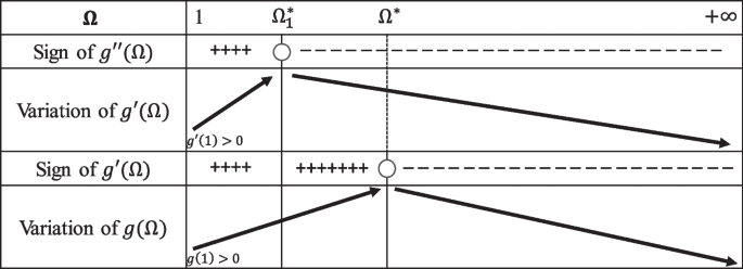
Table of variation for the function ${\text{g}}\left(\Omega \right)$ in the interval $\left(1,+\infty \right)$ for the case:$-27/8 \le {\text{c}}<\frac{27\left(\upbeta -7\right)}{2\left(11\upbeta +13\right)}$

Fig. 13

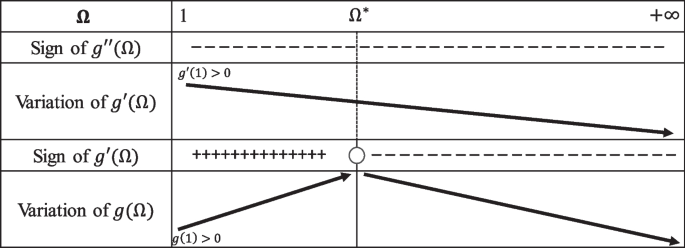
Table of variation for the function ${\text{g}}\left(\Omega \right)$ in the interval $\left(1,+\infty \right)$ for the case: $\frac{27\left(\upbeta -7\right)}{2\left(11\upbeta +13\right)}\le {\text{c}}\le \frac{27\left(\upbeta -4\right)}{2\left(11\upbeta +1\right)}$

Fig. 14

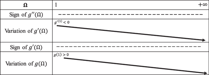
Table of variation for the function ${\text{g}}\left(\Omega \right)$ in the interval $\left(1,+\infty \right)$ for the case: $\frac{27\left(\upbeta -7\right)}{2\left(11\upbeta +13\right)} \le \mathrm{c }\le 2.25$

References

Banabic D (2000) Formability of metallic materials: plastic anisotropy, formability testing, forming limits. Springer Science & Business Media, Berlin
Corallo L, Mirone G, Verleysen P (2023) A novel high-speed bulge test to identify the large deformation behavior of sheet metals. Exp Mech 63:593–607. https://doi.org/10.1007/s11340-022-00936-5
DIN EN ISO 16808:2014 (2014) Metallic materials—sheet and strip—determination of biaxial stress–strain curve by means of bulge test with optical measuring systems. BSI. https://www.iso.org/standard/57777.html
DIN EN ISO 16808:2022 (2022) Metallic materials—sheet and strip—determination of biaxial stress–strain curve by means of bulge test with optical measuring systems. BSI. https://www.iso.org/standard/82103.html
Alharthi H, Hazra S, Alghamdi A, Banabic D, Dashwood R (2018) Determination of the yield loci of four sheet materials (AA6111-T4, AC600, DX54D+ Z, and H220BD+ Z) by using uniaxial tensile and hydraulic bulge tests. The International Journal of Advanced Manufacturing Technology 98:1307–1319
Mulder J, Vegter H, Aretz H, Keller S, van den Boogaard AH (2015) Accurate determination of flow curves using the bulge test with optical measuring systems. J Mater Process Technol 226:169–187
Hill R (1948) A theory of the yielding and plastic flow of anisotropic metals. Proceedings of the Royal Society of London A 193:281–297. https://doi.org/10.1098/rspa.1948.0045
Cazacu O, Revil-Baudard B (2020) Plasticity of metallic materials: modeling and applications to forming. Elsevier, Amsterdam
Martins B, Santos AD, Teixeira P (2013) A study on the influence of different variables for determination of flow stress using hydraulic bulge test. International Journal of Materials Engineering Innovation 4(2):132–148
Khlif M, Mhadhbi M, Bradai C (2015) Development of bulge test for aluminum sheet metal. In: Chouchane M, Fakhfakh T, Daly H, Aifaoui N, Chaari F (eds) Design and modeling of mechanical systems - II. Lecture Notes in Mechanical Engineering. Springer, Cham. https://doi.org/10.1007/978-3-319-17527-0_33
Jocham D, Norz R, Volk W (2017) Strain rate sensitivity of DC06 for high strains under biaxial stress in hydraulic bulge test and under uniaxial stress in tensile test. IntJ Mater Form 10:453–461
Young R, Bird J, Duncan J (1981) An automated hydraulic bulge tester. J Appl Metalwork 2(1):11–18
Rees D (1995) Plastic flow in the elliptical bulge test. Int J Mech Sci 37(4):373–389
Rodrigues CA, Reis LC, Sakharova NA, et al (2012) On the characterization of the plastic behaviour of sheet metals with bulge tests: numerical simulation study. In: Eberhardsteiner J et al (ed) 6th Eur Congr Comput Methods Appl Sci Eng ECCOMAS. ECCOMAS 2012, Vienna, Austria, pp 4575–4589
von Mises R (1913) Mechanik der festen Körper im plastisch deformablen Zustand. Nachrichten von der Gesellschaft der Wissenschaften zu Göttingen, Mathematisch-Physikalische Klasse, pp 582–592
Kleiser G, Revil-Baudard B, Abrahms R, Martin B, Cazacu O (2017) Influence of processing on deformation and damage in high-strength steels, presented at the SEM XIII International Congress. FL, Orlando
Cazacu O, Plunkett B, Barlat F (2006) Orthotropic yield criterion for hexagonal closed packed metals. Int J Plast 22(7):1171–1194
Drucker DC (1948) The Relation of Experiments to Mathematical Theories of Plasticity. Brown University, Division of Applied Mathematics
Green AE, Naghdi PM (1965) A general theory of an elastic-plastic continuum. Arch Ration Mech Anal 18(4):251–281
Cazacu O, Revil-Baudard B, Chandola N (2019) Plasticity-damage couplings: from single crystal to polycrystalline materials. Springer, Cham
Abaqus (2014) Abaqus - Version 6.14–1. Dassault Systemes Simulia Corp., Providence, RI
Author information
Authors and Affiliations
Corresponding author
Ethics declarations
Competing interests
The authors have no competing interests to declare that are relevant to the content of this article.
Additional information
Publisher's Note
Springer Nature remains neutral with regard to jurisdictional claims in published maps and institutional affiliations.