Abstract
Various industries and fields have utilized machine learning models, particularly those that demand a significant degree of accountability and transparency. With the introduction of the General Data Protection Regulation (GDPR), it has become imperative for machine learning model predictions to be both plausible and verifiable. One approach to explaining these predictions involves assigning an importance score to each input element. Another category aims to quantify the importance of human-understandable concepts to explain global and local model behaviours. The way concepts are constructed in such concept-based explanation techniques lacks inherent interpretability. Additionally, the magnitude and diversity of the discovered concepts make it difficult for machine learning practitioners to comprehend and make sense of the concept space. To this end, we introduce ConceptGlassbox, a novel local explanation framework that seeks to learn high-level transparent concept definitions. Our approach leverages human knowledge and feedback to facilitate the acquisition of concepts with minimal human labelling effort. The ConceptGlassbox learns concepts consistent with the user’s understanding of a concept’s meaning. It then dissects the evidence for the prediction by identifying the key concepts the black-box model uses to arrive at its decision regarding the instance being explained. Additionally, ConceptGlassbox produces counterfactual explanations, proposing the smallest changes to the instance’s concept-based explanation that would result in a counterfactual decision as specified by the user. Our systematic experiments confirm that ConceptGlassbox successfully discovers relevant and comprehensible concepts that are important for neural network predictions.
Introduction
Deep learning has resulted in significant breakthroughs in various domains, including natural language processing, speech recognition, medical applications, computer vision, and autonomous vehicles [1,2,3,4,5]. The complexity and intrinsic opaqueness of neural networks that includes hundreds of millions of parameters with extremely non-linear transformations, makes comprehending model behaviour and inner workings challenging. As a result, the focus on deep learning has recently shifted from model performance to model interpretability. In light of the European Parliament’s enactment of the general data protection regulation (GDPR) in May 2018, interpretability has gained significant prominence, particularly with respect to the requirement for industries to provide explanations for any decision made through automated decision-making. The GDPR mandates that individuals have the right to obtain meaningful explanations regarding the logic involved in such decisions [6].
Generally, the interpretability of deep learning models is achieved by two approaches. The first approach focuses on making the inner logic and algorithmic functions of the model transparent, which requires users to have deep learning expertise, and thus inappropriate as a paradigm for non-experts [7]. The second approach uses transparent models to approximate the behaviour of the neural network on a task [8]. This approach is appropriate for non-experts users, but it should be carefully employed as it comes with inherent information loss and potentially false reflection [9]. One possible neural networks (NNs) explanation approach for non-experts is to visualize the inner working of NN by demonstrating how perturbing the input affects model outputs. For example, in an image classification task, saliency and activation maps measure the importance of the input features (i.e., image pixels) to the model in classifying an image [10,11,12,13,14]. The major limitation of such heatmap explanation techniques is that they do not provide sufficient information to elucidate the primary factors behind a specific prediction.
Consequently, a recent line of research has emerged that concentrates on the automatic extraction of concepts [15, 16]. This research aims to identify meaningful high-level concepts that are critical for model prediction, and then break down the evidence supporting the prediction into importance scores for the extracted concepts. Although concepts-based interpretability techniques are appropriate for non-experts, there has yet to be a limited application, mainly due to common difficulties that make concept generation and presentation difficult. While these techniques support the automatic extraction of interpretable concepts, they do not incorporate human-in-the-loop, making it challenging for users to get the concepts to align with their intuitive representation of the problem.
To address the previously mentioned challenge, we opt for a strategy known as interactive concept learning that allows end-users to interactively train machine learning models to identify desired concepts. Designing for effective end-user involvement with a model as it learns and refines its definition of a concept is a key difficulty in end-user interactive concept learning. This work is an extension of our initial work [16] that mainly focused on automatically extracting concepts to provide local explanations for classification networks. In this work, we focus on turning features learnt from the convolutional neural network into intuitive concepts that users can readily reason about and then explain the prediction in terms of these concepts. Our aim is to develop a two-stage prediction framework. In the initial stage, a concept definition function is employed to map the embeddings of the image being explained to relevant concepts. Subsequently, these concepts are utilized by a secondary function to generate predictions derived from the model being explained. Our goal is to refine the interpretability of this secondary function, ensuring it remains locally faithful to the model being explained. Concurrently, we seek to iteratively train the first function to align with the user’s conceptual understanding, thereby enhancing the interpretability of the entire prediction process. We summarize our contributions as follows:
-
We introduce ConceptGlassbox, an innovative framework for providing local explanations that facilitates the acquisition of transparent and high-level concept definitions that captures the user’s mental model to explain deep learning models. Central to our proposal is active learning, where human knowledge and feedback are integrated to learn intuitive concepts with little human labelling effort.
-
ConceptGlassbox provides counterfactual explanations, suggesting the minimal adjustments within the instance’s concept-based explanation required to achieve a user-defined counterfactual decision.
-
Quantitative human experiments and evaluations demonstrate the superiority of ConceptGlassbox. Participants favored ConceptGlassbox-derived concepts, with 90% selecting them as more meaningful compared to baseline methods. In comparison to the Interpretable Basis Decomposition (IBD) technique [17], ConceptGlassbox demonstrates superior performance, with 82% of participants identifying ConceptGlassbox-derived concepts as the most significant contributors to model predictions, as opposed to 60% for IBD. Additionally, ConceptGlassbox’s identified concepts enabled accurate human prediction in 96% of cases, highlighting its effectiveness in enhancing model interpretability.
Related Work
Recently, there has been a significant increase in the number of techniques for explaining the decisions made by machine learning models [18]. These techniques can be broadly divided into two categories: global and local [19]. Global techniques focus on the overall functioning of the prediction model, while local techniques promote the understanding of small parts of the conditional distribution for specific instances [20,21,22,23]. Additionally, interpretability techniques can also be categorized based on the problem they solve [24]. The achievement of intrinsic interpretability involves constructing self-explanatory models that inherently possess interpretability by design. Conversely, post-hoc interpretability involves developing an additional model to explain an existing model. To attain intrinsic interpretability, models must be constructed with a self-explanatory design that directly incorporates interpretability into their structures. In contrast, post-hoc interpretability necessitates the construction of an additional model to explain an already existing model. The trade-off between these two categories is the balance between the model’s performance and the fidelity of the explanation.
As deep neural networks (DNNs) have achieved success in various fields [25], there has been a growing interest in developing methods for explaining these models. Such methods achieve interpretation by a variety of post-hoc and inherently interpretable techniques. Prototype-based interpretability is directly present in the model’s inner computations. ProtoPNet is the original work that uses class-specific prototypes for interpretable image classification tasks [26]. TesNet shares similarities with ProtoPNet by creating class-specific transparent basis concepts on the Grassmann manifold for interpretable classification [27]. Deformable ProtoPNet [28], which is derived from ProtoPNet, makes use of spatially-flexible and deformable prototypes to capture significant object features. While such prototype-based interpretability techniques are inherently interpretable, they could be time-consuming, and currently, there is no clear solution for combining them with popular architectures. Our proposed approach focuses on explaining already trained models without the need for retraining.
Post-hoc interpretability techniques can help to shed light on the decision-making process of DNNs. One category of post-hoc interpretability techniques for DNNs focus on visualizing the inner workings of DNNs and understanding their predictions by sampling patches that maximize the activations of hidden units [29], and backpropagation to identify the salient features in an image that have contributed to a particular prediction [13, 14, 30, 31]. Despite being widely employed, heatmap explanation techniques have faced criticism for their lack of informative value when attempting to gain a full understanding of the underlying reasons for a particular prediction. Another category highlights the most important features that contributed to a prediction by either removing [32, 33] or perturbing individual features to approximate their contribution [21, 23, 34]. However, these “feature-based” explanation techniques have their own limitations and are prone to human biases [35, 36]. They are also susceptible to minor shifts in the input, and human experiments have demonstrated that they do not enhance trust in the black-box model [37].
Consequently, another line of research focused on giving explanations in the form of concepts that are easy to understand [17, 37,38,39]. However, the main drawback of these concept-based techniques is that they give explanations based on what concepts the user is interested in rather than identifying the most significant concepts for the prediction that the user may not be aware of. Specifically, these methods require users to supply a set of examples that have been labelled by hand for each concept of interest and query the significance of each concept for the prediction. While these methods can be advantageous and offer useful insights, especially when the user has a precise set of concepts in mind and ample examples for each one, the main challenge with these techniques is the vast array of possible meaningful concepts that could be explored, making it difficult to provide sufficient examples for each of these concepts. Additionally, asking about a specific set of concepts may result in a biased explanation process that focuses on the provided concepts rather than identifying the correct set of concepts. In response to these challenges, an alternative set of techniques have emerged that aim to automatically identify high-level concepts that are significant for the model prediction. These techniques subsequently break down the evidence for a given prediction into a distinct importance score for each of the identified concepts [3, 15, 16]. While these methods facilitate the automated extraction of meaningful concepts, they often overlook user feedback, which can hinder users in obtaining concepts that resonate with their intuitive grasp of the problem.
Framework for Guided Concept-Based Interpretability
In Fig. 1, the process of explaining individual predictions is presented. It distinctly illustrates that when explanations are conveyed in terms of concepts that correspond with a user’s understanding of those concepts, it enables the user to make more informed decisions with the assistance of a machine learning model. In the following, we present ConceptGlassbox, a novel framework for local interpretability that facilitates the interactive acquisition of transparent and high-level concept definitions in the latent space and provide an explanation in the form of a small set of concepts contributing to the prediction of the instance being explained. The primary goal of ConceptGlassbox is to create an interpretable model over the learned concepts that is faithful to the black-box model.

Explaining individual predictions. a A set of images similar to the image being explained is retrieved. b Each image is segmented resulting in a pool of segments all coming from similar images to the one being explained. The activation space of one bottleneck layer of a state-of-the-art CNN classifier is used as a similarity space. Similar segments are clustered in the activation space and outliers are removed to increase coherency of clusters. c ConceptGlassbox incorporate the user feedback in forming high-level intuitive concepts. d ConceptGlassbox builds an interpretable model on the learnt concepts and highlights the intuitive concepts learnt from the interpretable model that led to the explanation of the instance being explained
Fidelity-Interpretability Trade-Off
Let \(x'\in \mathbb {R}^{d}\) be the initial representation of an instance being explained. More specifically, we adopt a perspective whereby an explanation is represented by a model \(f\in F\), selected from a class of inherently interpretable models including but not limited to linear models and decision trees. Model f is constructed over high-level intuitive concepts. Throughout this work, we will refer to the model to be explained as z. For classification task, \(z(x')\) is the probability of the membership of instance \(x'\) to a particular class. To define locality around \(x'\), we use \(\pi _{x'}(t)\) as a proximity measure between an instance t to \(x'\). Additionally, let \(L(z, f, \pi _{x'})\) be a measure of how inaccurate the approximation of z by f is in the locality specified by \(\pi _{x'}\). We also introduce a complexity measure \(\Omega \) for the explanation model f. For example, \(\Omega (f)\) could be the number of non-zero weights in the case of a linear model or the depth of the tree in case of a decision tree. To ensure that the explanation is both interpretable and locally faithful, we must minimize \(L(z, f, \pi _{x'})\) while keeping \(\Omega (f)\) low enough to be easily interpretable by humans. The explanation produced by ConceptGlassbox is obtained as follows:
Our objective is to train a two-stage prediction function, denoted as f, aimed at approximating the behavior of z in the proximity of \(x'\), leveraging a training dataset \(\{x_{n},y_{n}\}^{N}\), where x represents the input feature vector, and y corresponds to the prediction made by z. The first stage of the prediction function involves a concept definition function denoted as g, which maps the embeddings of x to binary concepts \(c\in \{0,1\}^{n}\). The second function, f, maps these concepts to predictions y obtained from z. Our objective is to obtain an interpretable function f that is locally faithful to z while also interactively training g to model the user’s knowledge about concepts.
Sampling for Local Exploration
We aim to minimize the locality-aware loss \(L(z,f,\pi _{x'})\) outlined in Eq. 1. To approximate the behavior of z in the vicinity of \(x'\), we estimate \(L(z,f,\pi _{x'})\) by drawing weighted samples by \(\pi _{x'}\). Specifically, we randomly select a set of instances \(I_{x'}\) from \(\{x_{n},y_{n}\}^{N}\) and assign weights to each sample instance based on its proximity to \(x'\) (See Fig. 1(a)). Instances in the vicinity of \(x'\) are assigned a higher weight, while those farther away receive a lower weight. In this work, we set the size of the sample \(I_{x'}\) to 500, deferring the exploration of a dynamic sample size to future work. Using the dataset \(I_{x'}\), we optimize Eq. 1 to derive an explanation \(\zeta (x')\). ConceptGlassbox framework generates a locally faithful explanation, where the notion of locality is encapsulated by \(\pi _{x'}\).
Automatic Concept Discovery
The main goal of the concept extraction phase is to automatically extract meaningful concepts that will be later refined through user feedback. ConceptGlassbox takes a trained classifier and an image to be explained. It then extracts the concepts present in \(I_{x'}\), where in image data, concepts are typically in the form of segments. To extract concepts from \(I_{x'}\), ConceptGlassbox starts with the segmentation of each image using semantic image segmentation technique that aims to assign a meaningful class to each pixel (See Fig. 1(b)). ConceptGlassbox uses DeepLabv3+ segmentation technique [40], which has been widely used due to its superior performance on dense datasets (after examining several segmentation techniques). To ensure the meaningfulness of the extracted concepts, we cluster segments into a number of clusters such that segments of the same cluster represent a particular concept. We define the similarity between segments as the Euclidean distance between their corresponding activation maps obtained from the intermediate layer of model z. Each segment was resized to the original size of z. All segments were passed through z to obtain their layer presentations and then clustered using the MeanShift clustering algorithm [41]. Then, we retain only the top \(n = 70\) segments within each cluster, selected based on their smallest Euclidean distance from the cluster center, while discarding the remaining segments. We exclude two types of clusters. The first type comprises clusters consisting of segments sourced from only one image or a very small number of images. These clusters pose an issue as they represent uncommon concepts within the target class. For example, if numerous segments of the same type of tree appear in just one image, they may form a cluster due to their similarity. However, such clusters do not represent common concepts in the dataset. The second type encompasses clusters containing fewer than L segments. In this work, we use constant value for L equals \(0.4\sqrt{n_c}\), where \({n_c}\) is the number of segments in cluster c, leaving the exploration of different values for L to future work. The main problem with clusters of few segments is that the concepts they present are uncommon in the neighborhood of the image being explained. To achieve a balance, we maintain three categories of clusters: a) high-frequency (segments appearing in over half of the discovery images), b) medium-frequency with moderate popularity (appearing in more than one-quarter of discovery images and with a cluster size larger than the number of discovery images), and c) high popularity (cluster size exceeding twice the number of discovery images). The output of this phase is a set of clusters represent the learnt concepts denoted \(C=\{c_1,...c_n\}\) with centers \(\{s_{c_1},...s_{c_n}\}\), where n is the number of concept clusters after the exclusion criteria.
Interactive Concept Learning
To learn g that maps the embeddings of x to \(c\in \{ 0,1\}^{n}\), we do the following. For each segment, \(s\in c\), the hidden layer activations \(a=z_{l}(s)\) at layer l is extracted and stored along its corresponding concept label. For each candidate concept \(c\in C\), we train a logistic binary classifier \(h_{c}\) to detect the presence of concept c. First, we proceed to train each concept denoted as c on the dataset \(D_{c}\), which comprises a combination of segments carefully balanced to include instances both with and without the presence of concept c. We define \(D_{c}=D^{+}_{c} \cup D^{-}_{c}\), where \(D^{+}_{c}=\{(z_{l}(s^{1}),y_{c}^{1}),...., (z_{l}(s^{|c|}),y_{c}^{|c|})|_{y_{c}=1}\}\) and \(D^{-}_{c}=\{(z_{l}(s^{1}),y_{c}^{1}),...., (z_{l}(s^{|c|}),y_{c}^{|c|})|_{y_{c}=0}\}\), where \(y_{c}\in \{0,1\}\) indicates the absence or the presence of concept c in a segment. Negative examples \(D^{-}_{c}\) for each concept c are randomly selected from other cluster concepts such that the number of examples in \(D^{+}_{c}\) and \(D^{-}_{c}\) are equal. We use these concept classifiers for each image \(I_{x'}^{i} \in I_{x'}\) to create a binary vector \(v=(r_{1}, r_{2},..., r_{n})\) representing the presence or absence of each concept \(c\in C\) in \(I_{x'}^{i}\), where \(r_{i}=h_{c_{i}}(I_{x'}^{i})\), \(r_{i}\in \{0,1\}\).
To incorporate the user’s knowledge in learning function g, we interactively learn the representative set of segments associated with each concept. On the one hand, asking the user for the intuitiveness of each segment in each cluster results in a frustrating experience that treats the user as a mere information oracle. On the other side, a design that ignores the needs of the machine learning model in favour of end-user flexibility may be equally frustrating if a user cannot properly train the model to recognize a desired concept. To assist a user in effectively steering a machine learning model while preserving the user’s flexibility and controllability, we cluster all segments in each cluster \(c_{i}\) using k-means clustering algorithms [42]. In this work, we employ a static value of k, specifically \(k = 15\), leaving the investigation of alternative values for future research. This phase yields d clusters \(C' =\{c'_{1},..., c'_{d}\}\) with centres \(\{s'_{1}, s '_{2},... s'_{d}\}\), where d is the total number of clusters obtained from the k-means algorithm applied on C. Next, the user is asked whether a segment \( s'_{i}\) should be associated with concept \(c_{j}\). It is posited that the intuitiveness of function g is achieved when the user acknowledges the suggested association between segments in a particular cluster \(c'_{i}\) represented by a segment \( s'_{i}\) and a concept \(c_{j}\) for every (i, j) cluster-concept association in g. To learn g that satisfies intuitiveness, we do the following. We define a binary matrix \(A\in \{0,1\}^{d\times n}\), \(A_{i,j}=1\) represents the association of segments in cluster \(c'_{i}\) to concept j and \(A_{i,j}=0\) represents the dissociation of cluster \(c'_{i}\) from concept j. We first initialize matrix, A, by associating cluster \(c'_{i}\) containing segment \(s_{c_j}\) to concept \(c_{j}\). Algorithm 1, which is adapted from [43], outlines the procedure for associating clusters to concepts. The algorithm constructs g on \(C'\) incrementally by suggesting several cluster-concept proposals \((i^*,j^*)\) that the user either accepts or rejects. The algorithm generates proposals based on pairs of (i, j) that have not been previously explored. A predetermined number of proposals are produced for each concept before proceeding to the subsequent one. In this work, we utilize a constant number of proposals per concept, which is denoted as \(numproposals=10\). More specifically, each concept \(c_j\) is associated with two feature lists. The first is the explored list \(l_{j}\), which includes the clusters that have been suggested to users as possible associations with the concept \(c_j\). The second is the unexplored list \(u_{j}\), which contains the set of clusters that have not yet been proposed for concept \(c_j\).
If a user approves the proposed cluster-concept pairing, the proposed cluster is incorporated into the definition of the concept, resulting in the cluster-concept matrix being updated such that \(A_{i,j}=1\). If the user rejects the proposal, the matrix remains unchanged. Initially, list \(l_{j}\) is initialized with a single cluster i, whereby \(A_{i,j}=1\) for all concepts j, while \(u_{j}\) contains the remaining clusters not included in \(l_{j}\). Algorithm 1 outlines the process of modelling user feedback and proposing cluster-concept associations. The algorithm adapts its proposals based on the user’s prior acceptance of proposed associations, and iteratively refits model f after each update to function g. To do so, a matrix intuit is maintained to store the labels of the proposals that have been accepted or rejected by the user. This matrix is initialized with \(intuit_{i,j}=1\) and \(intuit_{i,j'\ne j}=0\), if \(A_{i,j}=1\) in the concept definitions initialized by the user. If a user agrees with the suggested cluster-concept association, the matrix is updated by setting \(intuit_{i^*,j^*}\) to 1. However, if the user disagrees, the matrix remains unchanged. It is noteworthy that a given cluster may be associated to multiple concepts. The primary challenge is to suggest cluster-concept associations that are both faithful to the model and intuitive to the user. If the proposal accurately reflects the black-box model but is not intuitive to the user, it will not be accepted, and the overall performance of f will not improve. Conversely, if a proposal is unfaithful, even if accepted by the user, it will not enhance the performance of f. Therefore, the objective is is to generate a substantial number of proposals that exhibit interpretability while maintaining a high level of predictive accuracy. To accomplish this goal, two scores are computed for each proposal: fidelity score (SFid) and intuitiveness score (SIntuit). \(SFid_{i,j}\) is used to assess the degree to which model f accurately captures the behavior of z in the vicinity of \(x'\) when associating cluster i to concept j.
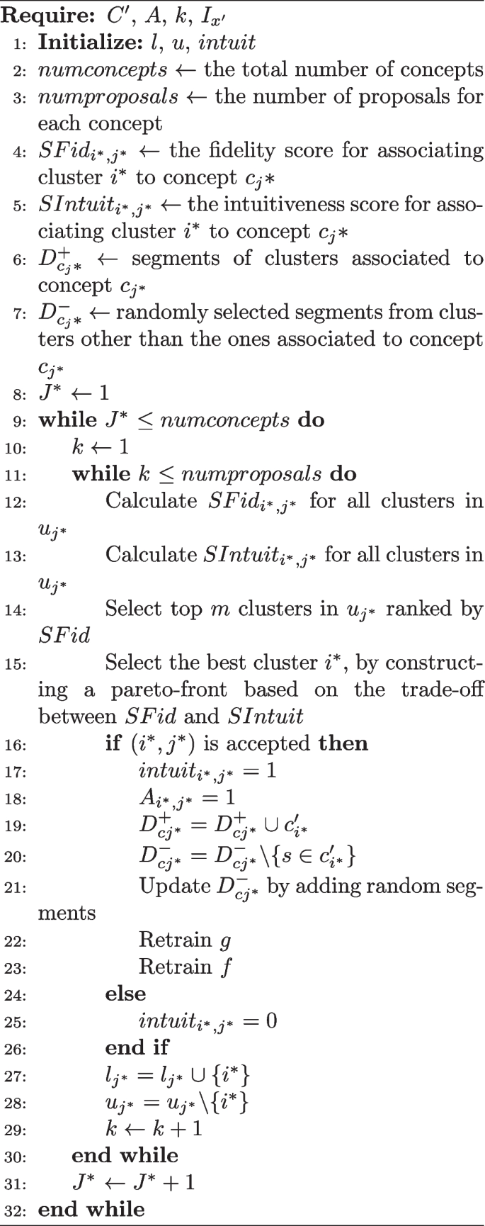
Algorithm for interactively proposing intuitive and interpretable concepts with human feedback
\(SFid_{i,j}\) is calculated for each concept \(c_j\), and the scores are ranked to prioritize proposals that enhance the fidelity of the model. The \(SFid_{i,j}\) score is computed by updating the value of f once the user approves the (i, j) proposal. Our objective with \(SIntuit_{i,j}\) is to evaluate the likelihood of the user accepting the association between cluster i and concept j. We calculate \(SIntuit_{i,j}\) for each concept \(c_j\) and prioritize our proposals based on the ranking of these scores to increase the chances of acceptance by the user. To achieve coherence in our concepts, we assume that the user is more inclined to approve the association of cluster i with concept j if another similar cluster i′ has already been associated to concept j. The notion of similarity between two clusters is defined by the Euclidean distance (denoted D) between the centres of the two clusters. We determine the likelihood of the user accepting the association between cluster i to concept j as follows:
Our objective is to produce cluster-concept proposals that are both highly intuitive and faithful. To achieve this, we rank the proposals based on the Pareto front of the trade-off between intuitiveness and fidelity, selecting the one with the highest rank.

A shallow concept-based explanation decision tree, with a depth of 4, is employed to elucidate the prediction of an image depicting the coastline
Constructing Local Explanation
ConceptGlassbox constructs the explanation model over a dataset consisting of the concept representation v for each image \(I^i_{x}\in \) \(I_{x}\) along with the class prediction obtained from z. ConceptGlassbox is based on the view that a satisfactory explanation should explain both the prediction of the instance being explained and a user-defined counterfactual decision. The ConceptGlassbox framework employs two distinct explanation models for explaining instances in terms of high-level concepts. Moreover, ConceptGlassbox offers a counterfactual explanation, which delineates the minimal alteration required in the feature values to transition the prediction to a predefined output [44]. The first model is a decision tree classifier favoured for its interpretability. It allows for deriving concept rules from a decision tree’s root-leaf path and extracting counterfactuals via symbolic reasoning. To swiftly search for counterfactuals, the framework considers all possible paths in the decision tree that result in a user-specified decision. The one with the least number of unsatisfied split conditions by \(x'\) is selected from these paths. As the depth of the decision tree increases, its prediction accuracy improves, but its interpretability decreases as the number of nodes grow rapidly. Therefore, a shallow decision tree is favored due to its enhanced comprehensibility. In this work, a fixed depth of 4 is used, with the investigation of dynamic depth left for future work. Figure 2 illustrates an explanation tree for an image predicted as a coast. The explanation tree indicates that the image has been classified as a coast due to the presence of concepts ‘mountain’, and ‘sea’. ConceptGlassbox provides a counterfactual explanation for a user-defined counterfactual decision (i.e., snowy mountain), which is the path in the decision tree that results from the presence of concepts ‘mountain’, ‘sea’, and ‘tree’ leading to snowy mountain prediction for the instance being explained. The second explanation model used by ConceptGlassbox is logistic regression, favoured for its interpretability through concept weights. To obtain a counterfactual explanation using a logistic regression model, the following approach is taken. Firstly, the concept representation \(x''\) of the instance being explained \(x'\) is obtained. Let \(min_{c}(x'')\) be the vector obtained by modifying the minimum number of concepts in \(x''\) such that \(f(min_{c}(x''))=y'\) and \(f(x')=y\), where \(y'\) is a user-specified counterfactual decision and \(y\ne \) \(y'\). A perturbation of \(x'\) is the minimum change in the number of concepts to change the prediction of \(x'\) to \(y'\). We calculate all perturbations of \(x'\) and select the perturbation that exhibits the highest probability of class \(y'\).
Results and Discussion
Experimental Setup
Model and Dataset
We use ConceptGlassbox to explain the predictions of Resnet50 trained on ADE20K dataset [45]. We select a subset of 30 classes out of the 150 classes from ADE20K dataset. The dataset utilized in this study is divided into three subsets: 60% for training, 20% for validation, and 20% for testing.
Baseline
To provide explanations for individual predictions, we compare ConceptGlass-box against different baseline methods. The interactive baseline, denoted as AL, employs the same function f as ConceptGlass-box, which is trained on top of concepts, but uses a different concept definition function g. To simulate user feedback on cluster-concept associations, we need to model the user interaction of the baseline. Specifically, AL fits binary logistic classifiers on each cluster \(c_{i}\in C\) on \(D_{c_{i}}=D_{c_{i}}^{+} \cup D_{c_{i}}^{-}\). For each instance x within the set \(I_{x'}\), we employ the concept classifiers to generate a vector \(x_{AL}=(r_{1}, r_{2},..., r_{n})\), where each element \(r_i\) represents the probability associated with the presence of concept \(c_{i}\) in this particular instance [16]. Subsequently, we utilize these concept vectors, derived from instances in \(I_{x'}\), directly during the training of unregularized logistic regression and shallow decision trees. User feedback is communicated by assigning concept labels to instances. The non-interactive baselines do not not utilize concepts and simply compares to regularized logistic regression (LR), random forest classifier (RF), and a neural network (NN). The random forest model compromises 200 estimators, and the maximum depth of the trees was tuned using 10-fold cross-validation over the range of [5, 10, 25, 50]. The neural network uses ReLU activation function, ADAM as an optimizer and search overstep sizes from [0.001, 0,001, 0.01, 1]. We use a batch size of 32 and run it for 10000 iterations. All methods are trained using the scikit-learn implementations [41]. The final baseline entails a comparison with Interpretable Basis Decomposition (IBD) [17]. IBD is a method designed to deconstruct the prediction of an image into easily interpretable conceptual elements. It achieves this by decomposing the neural activations of the input image into an interpretable basis, which can be comprehended and analyzed by humans. Through this process, IBD uncovers the evidence encoded in the activation feature vector, thereby quantifying the contribution of each piece of evidence to the final prediction. This technique relies on human-provided examples of concepts. Leveraging the learned concepts C, we derive an interpretable basis to facilitate further analysis and understanding.
Comparison to Various Baselines
For each instance \(x'\) in the test set, we evaluate the performance of ConceptGlassbox and all baseline methods on \(I_{x'}\) samples, which are drawn from the training set and have their class labels obtained from ResNet50. Table 1 displays the mean balanced accuracies on downstream tasks, as well as the concept accuracies on the test set, for our proposed method and both the interactive and non-interactive baseline approaches. Downstream accuracy refers to the model’s performance on the final classification task, while concept accuracy evaluates the performance of the concept classifiers trained to detect the presence or absence of concepts in images. The results demonstrate that our approach outperforms the interactive concept-based baseline (AL) in terms of both concept accuracy and downstream accuracy, when the function f is either a decision tree or logistic regression. In particular, when f is a shallow decision tree, our approach achieves a final concept accuracy of \(96\% \pm 0.001\), which is \(6\%\) higher than that of the AL baseline. This significant improvement indicates that our proposed approach is much more aligned with intuitive user representation than the baseline approach. Our method outperforms the LR baseline and offers an advantage as users determine the concepts utilized in our approach. In contrast, LR does not have any restrictions on the intuitiveness or colinearity of its inputs. Compared to non-interpretable methods, our proposed approach outperforms RF by 2%, while NN slightly outperforms our approach by only 1%.
Examining the Significance of the Extracted Concepts from ConceptGlassbox
We compare the average accuracy of our approach (using the decision tree variant) to randomly associating clusters to concepts as if a user were manually generating g (See Fig. 3). The x-axis shows the number of cluster-concept proposals per concept. The results of our approach are based on 6, 8, and 10 proposals. The results show that associating random clusters to concepts does not come close to the performance of our proposed approach, as depicted in Fig. 3.

Downstream accuracy of our approach using decision tree variant against randomly selected features from the concept definitions
Faithfullness of the Explanations of ConceptGlassbox
The following metrics are utilized to assess the degree to which the decision inferred by the explanation model f and the explanations obtained from ConceptGlassbox mimic the behaviour of the black-box model.
-
Fidelity \(\in [0,1]\): measures the degree to which an explanation accurately represents the underlying model’s behavior. Essentially, it evaluates how well the explanation reflects the true reasoning of the model. Specifically, fidelity compares the predictions of models f and z on the image set \(I_{x'}\) to explain instance \(x'\) [46]. High fidelity indicates that the explanation accurately captures the model’s behavior, while low fidelity suggests that the explanation may not fully represent the model’s decision-making process.
-
Hit \(\in \{0,1\}\): evaluates the concordance between the predictions of two models, represented by f and z, on a given input instance \(x'\) [47]. The hit metric returns a binary outcome: a value of 1 signifies perfect agreement between the models’ predictions, indicating that both models yield identical predictions for the input instance \(x'\), while a value of 0 indicates a lack of concordance, signifying divergent predictions by the models.
We measure the fidelity by the f1-measure [48]. Aggregated values of f1 and hit are reported by averaging them over the set of instances in the testing dataset. The fidelity and the hit of ConceptGlassbox and the AL baseline are reported in Table 2. For ConceptGlassbox, we consider two explanation models; decision tree and logistic regression based on Lasso(using the regularization path [49]). The results show that ConceptGlassbox when f is a decision tree, achieves fidelity of \(97\% \pm 0.001\) and a hit of \(98\% \pm 0.002\), outperforming the AL baseline.
Importance of ConceptGlassbox Concepts
To confirm the importance of the concepts obtained by the ConceptGlassbox, we generalize the importance measure introduced for pixel importance scores in the literature [50] to the case of concepts. Specifically, we extend the notion of smallest sufficient concepts (SSC) to identify the minimum set of concepts required to predict the target class. To examine ConceptGlassbox with this measure, on 500 randomly selected instances from the testing dataset, we compare the prediction accuracy of Resnet50 (baseline) to the prediction accuracy of the explanation models supported by ConceptGlassbox as we add important concepts and when we randomly add concepts (random), as shown in Fig. 4. The results show that when f is a decision tree using the top-5 concepts is enough to reach 90% of the original accuracy of the Resnet50. When the explanation model is a sparse logistic regression, using top-5 concepts is enough to reach within 83% of the original accuracy of the Resnet50. The results also confirm that adding random concepts does not come close to the performance of ConceptGlassbox and AL baseline.

Prediction accuracy of the explanation models supported by ConceptGlassbox as adding the top K important concepts aggregated over randomly selected instances from the testing dataset

Average accuracy of all concept classifiers trained for main layers of ResNet50
Concept Classifier Prediction Performance
Concept models’ performance varies across the different layers of the main task model (ResNet50). To identify the best layer to extract feature vectors used to train concept classifiers, we compare the average accuracy of the concept models built on vectors extracted from the major layers of Resnet50 and report the performance averaged over all instances in the testing dataset. Major layers refer to the conv2 (layer1), conv3 (layer 2), conv4 (layer 3), and conv5 (layer 4) block sections of sublayers of Resnet50. Figure 5 shows that all layers have high average accuracy, and the deeper the extraction layer, the higher the accuracy. The average classifier accuracy was the highest at the fourth layer, achieving an accuracy of 0.98 (See Fig. 5).

Human evaluation interface for identifying meaningful concepts

Sample examples of human experiments for choosing the most contributing concept to their predictions

Stitching important concepts of four different images. List of five concepts are shown to the left of the concepts set and the right concept in shown below the image. For instance, bed, wall, cabinet and window seem to be enough for the ResNet50 to classify an image as a bedroom
Human Evaluation of the Visual Explanations
To measure the meaningfulness of the extracted concepts, we randomly select 50 instances from the testing dataset and get the concepts used in their explanations from ConceptGlassbox and AL baseline. We ask 30 human participants to identify the most meaningful set of segments that belong to a concept among concepts obtained from ConceptGlassbox and AL in addition to random set of segments. The evaluation interface is shown in Fig. 6. Results show that 90% of participants choose the concept obtained from ConceptGlassbox.
To measure the significance of concepts extracted from the ConceptGlassbox and IBD, we asked the 30 participants to select the most meaningful concept contributing to a particular prediction made by ResNet50 for 30 images. In each task, participants are presented with the image to be explained alongside its prediction, accompanied by four concepts. Among these, one concept corresponds to the top concept identified by ConceptGlassbox, utilizing a decision tree variant. Another concept denotes the top concept identified by IBD. The two remaining concepts are chosen randomly. If the top concepts of ConceptGlassbox and IBD are identical, one of them is selected along with three random concepts. Participants are asked to select the most meaningful concept (image) contributing to the prediction. Figure 7 shows two sample images along with four different concepts in which participants are asked to choose the most contributing concept for predicting these images. On average, 82% of participants selected the concept identified by ConceptGlassbox as the most significant. In cases where the top concepts from ConceptGlassbox and IBD were the same, they were counted for both techniques. Consequently, on average, 60% of participants identified the concept obtained through IBD as the most important.
Another natural question is whether the existence of the important concepts identified by ConceptGlassbox is enough for humans to predict the class of the instance to be explained without having the complete structural properties; an image of a ‘sofa’, ‘shelf’, ‘painting’and ‘window’is predicted as a living room. Participants are shown the top four important concepts identified by ConceptGlassbox on a blank image and are asked to choose the most relevant class for this image among five choices (one is correct, and the rest are randomly chosen). Figure 8 shows a sample of four sets of concepts and five choices. For 100 randomly selected images from 30 different classes, 96% images have been classified correctly.
Conclusion
We presented a novel interactive interpretability technique, ConceptExplanier, that provides intuitive concept-based explanations for classification networks. Our framework integrates human knowledge and feedback to learn high-level transparent concept definitions to train concept detector models with minimal human labelling effort. Such concepts are then used to explain the instance prediction through two interpretable models; logistic regression and shallow decision tree. Moreover, ConceptExplanier supported counterfactual explanations by identifying the minimum changes in the instance’s concept-based explanation that will lead to a user-defined counterfactual decision. Our results showed that the explanations provided by our approach were faithful to the underlying model. While our approach outperformed both interpretable and interactivee baseline, we cannot guarantee that our approach will always be able to learn concepts in diverse domains.
Data Availability
No datasets were generated or analysed during the current study.
References
Wang J, Pan M, He T, et al. A pseudo-relevance feedback framework combining relevance matching and semantic matching for information retrieval. Inf Process Manag. 2020;57(6):102342.
Komisarenko V, Voormansik K, Elshawi R, et al. Exploiting time series of Sentinel-1 and Sentinel-2 to detect grassland mowing events using deep learning with reject region. Sci Rep. 2022;12(1):983.
Shawi RE, Al-Mallah MH. Interpretable local concept-based explanation with human feedback to predict all-cause mortality. J Artif Intell Res. 2022;75:833–55.
Elshawi R, Sakr S. Automated machine learning: Techniques and frameworks. In: Big Data Management and Analytics: 9th European Summer School, eBISS 2019, Berlin, Germany, June 30–July 5, 2019, Revised Selected Papers 9. Springer; 2020. p. 40–9.
Alahdab F, El Shawi R, Ahmed AI, et al. Patient-level explainable machine learning to predict major adverse cardiovascular events from SPECT MPI and CCTA imaging. PLoS ONE. 2023;18(11):e0291451.
Goodman B, Flaxman S. European union regulations on algorithmic decision-making and a “right to explanation’’. AI Mag. 2017;38(3):50–7.
Liao QV, Gruen DM, Miller S, et al. Questioning the AI: informing design practices for explainable AI user experiences. In: Bernhaupt R, Mueller FF, Verweij D, et al., editors. CHI ’20: CHI Conference on Human Factors in Computing Systems. Honolulu: ACM; 2020. p. 1–15. https://doi.org/10.1145/3313831.3376590.
Gilpin LH, Bau D, Yuan BZ, et al. Explaining explanations: an overview of interpretability of machine learning. In: 2018 IEEE 5th International Conference on Data Science and Advanced Analytics (DSAA). IEEE; 2018. p. 80–9.
Došilović FK, Brčić M, Hlupić N. Explainable artificial intelligence: a survey. In: 2018 41st International Convention on Information and Communication Technology. IEEE: Electronics and Microelectronics (MIPRO); 2018. p. 0210–5.
Fong RC, Vedaldi A. Interpretable explanations of black boxes by meaningful perturbation. In: IEEE International Conference on Computer Vision, ICCV 2017. Venice: IEEE Computer Society; 2017. pp. 3449–57. https://doi.org/10.1109/ICCV.2017.371.
Saha A, Subramanya A, Patil K, et al. Role of spatial context in adversarial robustness for object detection. In: 2020 IEEE/CVF Conference on Computer Vision and Pattern Recognition, CVPR Workshops 2020. Seattle: Computer Vision Foundation/IEEE; 2020. pp. 3403–12. https://doi.org/10.1109/CVPRW50498.2020.00400.
Selvaraju RR, Cogswell M, Das A, et al. Grad-cam: Visual explanations from deep networks via gradient-based localization. In: IEEE International Conference on Computer Vision, ICCV 2017. Venice: IEEE Computer Society; 2017. pp. 618–26. https://doi.org/10.1109/ICCV.2017.74.
Simonyan K, Vedaldi A, Zisserman A. Deep inside convolutional networks: Visualising image classification models and saliency maps. arXiv:1312.6034 [Preprint]. 2013. http://arxiv.org/abs/1312.6034.
Zhou B, Khosla A, Lapedriza A, et al. Learning deep features for discriminative localization. In: 2016 IEEE Conference on Computer Vision and Pattern Recognition, CVPR 2016. Las Vegas: IEEE Computer Society; 2016. pp. 2921–9. https://doi.org/10.1109/CVPR.2016.31.
Ghorbani A, Wexler J, Zou J, et al. Towards automatic concept-based explanations. arXiv:1902.03129 [Preprint]. 2019b. Available from: http://arxiv.org/abs/1902.03129.
Shawi RE, Sherif Y, Sakr S. Towards automated concept-based decision tree-explanations for cnns. In: Velegrakis Y, Zeinalipour-Yazti D, Chrysanthis PK, et al., editors. Proceedings of the 24th International Conference on Extending Database Technology, EDBT 2021. Nicosia: OpenProceedings.org; 2021. pp. 379–84. https://doi.org/10.5441/002/EDBT.2021.38.
Zhou B, Sun Y, Bau D, et al. Interpretable basis decomposition for visual explanation. In: Ferrari V, Hebert M, Sminchisescu C, et al., editors. Computer Vision - ECCV 2018 - 15th European Conference. Munich, Germany, September 8-14, 2018, Proceedings, Part VIII, Lecture Notes in Computer Science, vol. 11212. Springer. pp. 122–38.
Bodria F, Giannotti F, Guidotti R et al. Benchmarking and survey of explanation methods for black box models. arXiv:2102.13076 [Preprint]. 2021. Available from: http://arxiv.org/abs/2102.13076.
Guidotti R, Monreale A, Ruggieri S, et al. A survey of methods for explaining black box models. ACM Comput Surv. 2018;51(5):93.
Plumb G, Molitor D, Talwalkar A, et al. Model agnostic supervised local explanations. In: Bengio S, Wallach HM, Larochelle H, et al., editors. Advances in Neural Information Processing Systems 31: Annual Conference on Neural Information Processing Systems 2018, NeurIPS 2018. Montréal; 2018. p. 2520–252.
Ribeiro MT, Singh S, Guestrin C. Why should I trust you?: Explaining the predictions of any classifier. In: Krishnapuram B, Shah M, Smola AJ, et al., editors. Proceedings of the 22nd ACM SIGKDD International Conference on Knowledge Discovery and Data Mining. San Francisco: ACM; 2016. pp. 1135–44. https://doi.org/10.1145/2939672.293977.
White A, Garcez AD. Measurable counterfactual local explanations for any classifier. arXiv:1908.03020 [Preprint]. 2019. Available from: http://arxiv.org/abs/1908.03020.
ElShawi R, Sherif Y, Al-Mallah M, et al. ILIME: local and global interpretable model-agnostic explainer of black-box decision. In: European Conference on Advances in Databases and Information Systems. Springer; 2019. p. 53–68.
Mohseni S, Zarei N, Ragan ED. A multidisciplinary survey and framework for design and evaluation of explainable AI systems. ACM Trans Interact Intell Syst (TiiS). 2021;11(3–4):1–45.
Domhan T, Springenberg JT, Hutter F. Speeding up automatic hyperparameter optimization of deep neural networks by extrapolation of learning curves. In: Yang Q, Wooldridge MJ, editors. Proceedings of the Twenty-Fourth International Joint Conference on Artificial Intelligence, IJCAI 2015. Buenos Aires: AAAI Press; 2015. pp. 3460–346.
Chen C, Li O, Tao D, et al. This looks like that: Deep learning for interpretable image recognition. In: Wallach HM, Larochelle H, Beygelzimer A, et al., editors. Advances in Neural Information Processing Systems 32: Annual Conference on Neural Information Processing Systems 2019, NeurIPS 2019. Vancouver; 2019. p. 8928–893.
Wang J, Liu H, Wang X, et al. Interpretable image recognition by constructing transparent embedding space. In: 2021 IEEE/CVF International Conference on Computer Vision, ICCV 2021. Montreal: IEEE; 2021. pp. 875–84. https://doi.org/10.1109/ICCV48922.2021.00093.
Donnelly J, Barnett AJ, Chen C. Deformable protopnet: An interpretable image classifier using deformable prototypes. In: IEEE/CVF Conference on Computer Vision and Pattern Recognition, CVPR 2022. New Orleans: IEEE; 2022. pp. 10255–1026.
Zeiler MD, Fergus R. Visualizing and understanding convolutional networks. In: European Conference on Computer Vision. Springer; 2014. p. 818–33.
Mahendran A, Vedaldi A. Understanding deep image representations by inverting them. In: IEEE Conference on Computer Vision and Pattern Recognition, CVPR 2015. Boston: IEEE Computer Society; 2015. pp. 5188–96. https://doi.org/10.1109/CVPR.2015.729915.
Selvaraju RR, Das A, Vedantam R, et al. Grad-CAM: Why did you say that? arXiv:1611.07450 [Preprint]. 2016. Available from: http://arxiv.org/abs/1611.07450.
Michie D, Spiegelhalter DJ, Taylor CC, Campbell J, editors. Machine learning, neural and statistical classification. Ellis Horwood; 1995.
Ribeiro MT, Singh S, Guestrin C. Model-agnostic interpretability of machine learning. arXiv:1606.05386 [Preprint]. 2016a. Available from: http://arxiv.org/abs/1606.05386.
Sundararajan M, Taly A, Yan Q. Axiomatic attribution for deep networks. arXiv:1703.01365 [Preprint]. 2017. Available from: http://arxiv.org/abs/1703.01365.
Ghorbani A, Abid A, Zou JY. Interpretation of neural networks is fragile. In: The Thirty-Third AAAI Conference on Artificial Intelligence, AAAI 2019, The Thirty-First Innovative Applications of Artificial Intelligence Conference, IAAI 2019, The Ninth AAAI Symposium on Educational Advances in Artificial Intelligence, EAAI 2019. Honolulu: AAAI Press; 2019. pp. 3681–8. https://doi.org/10.1609/AAAI.V33I01.3301368.
Gimenez JR, Ghorbani A, Zou J. Knockoffs for the mass: new feature importance statistics with false discovery guarantees. arXiv:1807.06214 [Preprint]. 2018. Available from: http://arxiv.org/abs/1807.06214.
Kim B, Wattenberg M, Gilmer J, et al. Interpretability beyond feature attribution: quantitative testing with concept activation vectors (TCAV). arXiv:1711.11279 [Preprint]. 2017. Available from: http://arxiv.org/abs/1711.11279.
Han S, Mao R, Cambria E. Hierarchical attention network for explainable depression detection on twitter aided by metaphor concept mappings. arXiv:2209.07494 [Preprint]. 2022. Available from: http://arxiv.org/abs/2209.07494.
Ge M, Mao R, Cambria E. Explainable metaphor identification inspired by conceptual metaphor theory. In: Thirty-Sixth AAAI Conference on Artificial Intelligence, AAAI 2022, Thirty-Fourth Conference on Innovative Applications of Artificial Intelligence, IAAI 2022, The Twelveth Symposium on Educational Advances in Artificial Intelligence, EAAI 2022 Virtual Event. AAAI Press; 2022. pp. 10681–1068.
Chen L, Zhu Y, Papandreou G, et al. Encoder-decoder with atrous separable convolution for semantic image segmentation. In: Ferrari V, Hebert M, Sminchisescu C, et al., editors. Computer Vision - ECCV 2018 - 15th European Conference, Munich, Germany, September 8-14, 2018, Proceedings, Part VII, Lecture Notes in Computer Science, vol. 11211. Springer; 2018. pp. 833–51. https://doi.org/10.1007/978-3-030-01234-2.
Pedregosa F, Varoquaux G, Gramfort A, et al. Scikit-learn: machine learning in python. J Mach Learn Res. 2011;12:2825–30.
Lloyd S. Least squares quantization in PCM. IEEE Trans Inf Theory. 1982;28(2):129–37.
Lage I, Doshi-Velez F. Learning interpretable concept-based models with human feedback. arXiv:2012.02898 [Preprint]. 2020. Available from: http://arxiv.org/abs/2012.02898.
Wachter S, Mittelstadt B, Russell C. Counterfactual explanations without opening the black box: automated decisions and the GDPR. Harv JL & Tech. 2017;31:841.
Zhou B, Zhao H, Puig X, et al. Scene parsing through ADE20K dataset. In: 2017 IEEE Conference on Computer Vision and Pattern Recognition, CVPR 2017. Honolulu: IEEE Computer Society; 2017. pp. 5122–30. https://doi.org/10.1109/CVPR.2017.544.
Doshi-Velez F, Kim B. Towards a rigorous science of interpretable machine learning. arXiv:1702.08608 [Preprint]. 2017. Available from: http://arxiv.org/abs/1702.08608.
Guidotti R, Monreale A, Ruggieri S, et al. Local rule-based explanations of black box decision systems. arXiv:1805.10820 [Preprint]. 2018a. Available from: http://arxiv.org/abs/1805.10820.
Olson DL, Delen D. Advanced data mining techniques. Springer Science & Business Media; 2008.
Efron B, Hastie T, Johnstone I, Tibshirani R. Least angle regression. 2004:407–99.
Dabkowski P, Gal Y. Real time image saliency for black box classifiers. Adv Neural Inf Process Syst. 2017;30.
Funding
This research has been funded by the project Increasing the knowledge intensity of Ida-Viru entrepreneurship co-funded by the European Union.
Author information
Authors and Affiliations
Contributions
Conceptualization, R.E.; methodology, R.E.; software,R.E; formal analysis R.E.; R.E. conducted the experiments; writing-original draftpreparation, R.E.; writing-review and editing, R.E.
Corresponding author
Ethics declarations
Ethical Approval
No ethical approval was required for this.
Competing Interests
The authors declare no competing interests.
Additional information
Publisher's Note
Springer Nature remains neutral with regard to jurisdictional claims in published maps and institutional affiliations.
Rights and permissions
Open Access This article is licensed under a Creative Commons Attribution 4.0 International License, which permits use, sharing, adaptation, distribution and reproduction in any medium or format, as long as you give appropriate credit to the original author(s) and the source, provide a link to the Creative Commons licence, and indicate if changes were made. The images or other third party material in this article are included in the article's Creative Commons licence, unless indicated otherwise in a credit line to the material. If material is not included in the article's Creative Commons licence and your intended use is not permitted by statutory regulation or exceeds the permitted use, you will need to obtain permission directly from the copyright holder. To view a copy of this licence, visit http://creativecommons.org/licenses/by/4.0/.
About this article

Cite this article
El Shawi, R. ConceptGlassbox: Guided Concept-Based Explanation for Deep Neural Networks. Cogn Comput (2024). https://doi.org/10.1007/s12559-024-10262-8
Received:
Accepted:
Published:
DOI: https://doi.org/10.1007/s12559-024-10262-8