Abstract
Clinicians often need to know if a new method of measurement is equivalent to an established one already in clinical use. This paper reviews the methodology of a method-comparison study to assist the clinician with the conduct and evaluation of such studies. Temperature data from one subject are used to illustrate the procedures. Although one would not make decisions based on the findings from one subject, the large number of paired measurements in the data set permits its use for illustrative purposes. Currently available software eliminates the need for tedious statistical computation, but does not reduce the burden of understanding the concepts underlying a method-comparison study and accurate interpretation of the findings.
Keywords: Bias, Clinical Measurement, Method-comparison, Precision, Temperature
With the rapid development and adoption of critical care technology, clinicians increasingly need to know if the newest technique is equivalent to that in current use. Such a question can be answered with a method-comparison study. For example, when noninvasive infrared thermometers were introduced, a plethora of studies was published reporting comparisons of body temperature values when measured simultaneously with the infrared thermometer and such established thermal sensors as the pulmonary artery catheter.1–5 Other examples of method-comparisons include arterial pulse contour versus pulmonary artery thermodilution cardiac output and point-of-care versus laboratory testing of blood glucose levels.6–8 The basic indication for a method-comparison study is the need to determine if two methods for measuring the same thing (e.g., body temperature, cardiac output) do so in an equivalent manner. The clinical question is one of substitution: Can one measure X with either Method A or Method B and get the same results?
In this paper the author discusses, and illustrates with two examples, the design, analysis and interpretation of a method-comparison study. The examples use partial data from a published report of in vitro and in vivo testing of multiple methods of measuring core body temperature in a pre-clinical critical care laboratory setting.9
Clinicians may wish to conduct a method-comparison study before adopting new technology in practice. This paper provides information on how to do so. At the very least, the information should help clinicians interpret the findings of method-comparison studies encountered in the literature.
Method-Comparison Methodology
A review of terminology precedes discussion of methodology as statistical reporting terms are used inconsistently in the literature.10 “Accuracy” and “precision” are used often when “bias” and “repeatability” are the properties being assessed. Accuracy is the degree to which an instrument measures the real value of a variable and is assessed by comparing the measurement method with a gold standard that has been calibrated to be highly accurate. In a method-comparison study, however, the investigator is comparing a less-established method with an established method already in clinical use. The difference in values obtained with the two methods represents the “bias” of the less established method relative to the more established one.
“Precision” is defined in two different ways: (1) the degree to which the same method produces the same results on repeated measurements, and (2) the degree to which values cluster around the mean of the distribution of values. The first definition equates with “repeatability:” How well does one method give the same results when measured over and over again? The second definition facilitates generalizing from the sample to the population by defining the range within which a value from the population is likely to fall. The closer together are the values within the range, the more precise is the estimate, and more confidence can be had in finding a result within that range in others who are like the sample, but not part of the sample.
Repeatability in a method-comparison study is a necessary, but insufficient, condition for agreement between methods. If one or both methods do not give repeatable results, assessment of agreement between methods is meaningless.
Design Considerations
Design issues for a method-comparison study include the selection of the measurement methods, timing of measurement, number of measurements and the range of physiological conditions over which the measurements are made. Each of these issues is briefly discussed.
Selection of Measurement Methods
It is intuitively obvious that the methods to be compared need to measure the same thing. For example, a bedside glucometer and a laboratory chemistry analyzer are both designed to measure blood glucose, and equivalence of these methods is appropriately assessed with a method-comparison study. In contrast, it is not appropriate to use method-comparison methodology to compare a pulse oximeter with a transcutaneous oxygen sensor, as the purpose of the pulse oximeter is to measure the percentage of hemoglobin saturated with oxygen, and the purpose of the transcutaneous sensor is to measure the partial pressure of oxygen in capillary blood. Although one may expect a strong correlation between the measurements, the methods are measuring different parameters of oxygenation. Thus, the first design step is to ensure that the two methods measure the same thing.
Timing of Measurement
The question being asked in a method-comparison study is can either of two different available methods be used to measure something equivalently. It follows that, to answer this question, the something (e.g., signal, biochemical value, physiological parameter) must be measured at the same time with the two methods. Thus, simultaneous sampling of the variable of interest is a requirement. The definition of “simultaneous” is determined by the rate of change of the variable. For example, body temperature is unlikely to change much over seconds or minutes and a sampling time difference of a few minutes is unlikely to affect the value obtained with Method A or Method B. In this case, one could design a study with sequential measurements. For example, measurement of tympanic temperature with an infrared thermometer could either precede or follow measurement with a pulmonary artery catheter thermal sensor. Simultaneous would then be defined as two measurements taken within several seconds of each other. A good design feature is to randomize the order of measurement so that any real time differences would be spread across the two methods of measurement. On the other hand, if one were to use sequential measurement under conditions of rapid change (e.g., malignant hyperthermia), measurements taken minutes apart are unlikely to be equivalent through no fault of the methods. Rather real changes in the temperature could explain differences in values. In such an instance, simultaneous measurements are indicated.
Number of Measurements
Paired measures are the sample of interest in a method-comparison study. Sample size determinations need to consider the number of paired measures sufficient to decrease chance findings. Large numbers of sets of paired measures and subjects add precision to the results and increase the likelihood that data will be normally distributed and, thus, validate the application of bias and precision statistics to the method-comparison. The number of subjects is determined during the design of the study. One way this can be done is with an a priori calculation using power (the probability of finding significance for the sample when a difference exists in the population), alpha (the level of significance selected before the statistical test is performed), and effect size (the smallest difference between the test methods that would be considered clinically important). This approach is illustrated in previously published reports.8, 11 An adequate sample size is particularly important in a method-comparison study where no difference is the hypothesized outcome. The investigator would be derelict in concluding that the test methods are interchangeable when the difference between methods would be significant with a larger sample size.
Conditions of Measurement
Most measurements used for acutely and critically ill patients need to be useful across a wide range of physiological conditions. For example, a thermometer that performs well only between 36 and 38°C is of limited use in patients with sepsis or fever. The design of a method-comparison study should allow for paired measurements across the physiological range of values for which the methods will be used. A large sample size and repeated measures across changing conditions over time can help the investigator achieve this design objective.
Analysis Procedures
Analysis procedures in a method-comparison study include the visual examination of data patterns with graphs and quantification of the estimate of the difference between methods and the precision of that difference, often referred to as bias and precision statistics (Definitions of terms used in method-comparison studies are provided in the table.). If the differences between methods are normally distributed, the investigator can, with a certain level of confidence, estimate the mean difference in patients like those who constituted the sample.
Table.
Definitions of terms used in a method-comparison study.
| Term | Definition |
|---|---|
| Bias | The mean (overall) difference in values obtained with two different methods of measurement |
| Confidence Limit | Range within which 95% of the differences from the bias are expected to be |
| Limits of Agreement | Confidence limits for the bias. Upper limit of agreement (Upper LOA in Figure 1) is computed as bias + 1.96SD, where SD is that of the bias. The lower limit of agreement (Lower LOA in Figure 1) is computed as bias − 1.96SD. Upper LOA − lower LOA = confidence limit |
| Percentage Error | Proportion between the magnitude of measurement and the error in measurement |
| Precision | The degree to which the same method produces the same results on repeated measurements (repeatability); the degree to which values cluster around the mean of the distribution of values (e.g., width of confidence interval) |
| Standard Deviation (SD) | A measure of variability of the individual differences |
Inspection of Data Patterns
The basic unit for analysis in a method-comparison study is the dyad of paired values. Examination of data patterns can be done with frequency distributions and scatter diagrams to inspect distribution of the data and relations between values obtained with the two methods. As with any type of study, the importance of closely inspecting the data before analysis cannot be over-emphasized. This step is often the first opportunity to note and eliminate outliers and artifacts and to assess the amount of missing data.
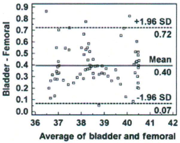
Bland and Altman recommended the use of plots, with bias and precision statistics, to determine agreement between methods.12–14 The Bland-Altman plot is easily constructed with the MedCalc software program (MedCalc®, Mariakerke, Belgium, http://www.medcalc.be/). The plot consists of the average of the paired values from each method on the x-axis and the difference of each pair of readings on the y-axis (Figure 1).
Figure 1.
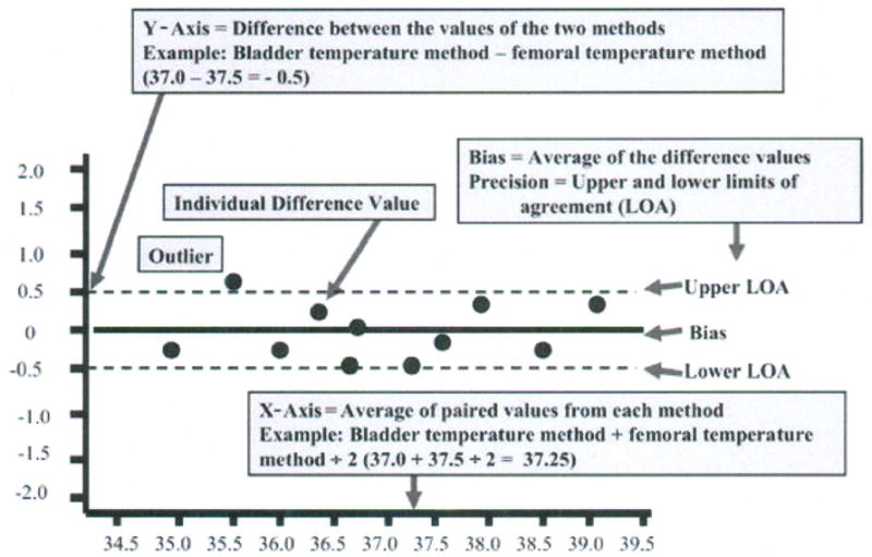
Structure of a Bland-Altman plot with explanation of elements, using a comparison of temperatures (degrees Centigrade) obtained with two temperature methods (bladder; femoral). (Modified and used with permission of M. Chulay).
Bias and Precision Statistics
The MedCalc program automatically calculates the bias and confidence limits for the bias (called the limits of agreement by Bland and Altman) and displays these as solid and dotted horizontal lines, respectively, on the graph as shown in Figure 1. The overall mean difference in values obtained with the two methods is called the bias. When the plotted differences represent the new method minus the established method, the bias quantifies how much higher (i.e., positive bias) or lower (i.e., negative bias) values are with the new method compared with the established one.
The standard deviation (SD) of all the individual differences is calculated as a measure of variability (repeatability) from which the limits of agreement are determined. The 95% confidence limits of the Normal distribution are used (mean difference ± 1.96 SD). The limits of agreement represent the range of values in which agreement between methods will lie for approximately 95% of the sample.
The Bland-Altman procedure assumes a linear relation between errors and measurements. This assumption is defensible for such measurements as temperature, but not for such other measurements as cardiac output and oxygen tension where the magnitude of error can have clinical consequences. A difference between two measurements (bias) of 0.5°C for temperature, for example, is no more clinically important for a temperature of 35°C than one of 39°C. However, a bias of 20 mmHg for PaO2 is more significant for a PaO2 of 60 mmHg than one of 100 mmHg. If the new method yields a PaO2 of 60 mmHg and the PaO2 with the established method was 40 mmHg, values from the new method would have serious consequences for patient safety and treatment. Likewise, a bias of 1 L/min for a cardiac output measure is more clinically significant at low cardiac outputs than at high ones. In other words, the magnitude of error needs to be considered across the range of physiological values for which the new method will be used. The Bland-Altman procedure considers the proportion between the magnitude of measurements and the error graphically, but not quantitatively. In other words, one can visualize proportional error from the Bland-Altman plot, but because the bias and repeatability estimates are computed across all of the data points, proportional error may not be apparent in the estimate. This problem can be handled by calculating the percentage error. The percentage error is derived by dividing the limits of agreement by the mean value of the measurements obtained with the established method.11 The criterion for acceptable percentage error will differ by the variable being measured.
The mean value of the measurement, the bias, the standard deviation of the difference, and the limits of agreement are reported and the Bland-Altman plot displayed as a graphic in presentation of the findings from a method-comparison study. Additionally, the percentage error should be included when the proportion of error to the magnitude of the measurement has clinical import.15
Interpretation of the Findings
Interpretation of the findings from a method-comparison study is straightforward. The clinically acceptable difference the investigator specified in the design phase is used to interpret the findings. The bias and precision results are compared to the a priori specifications. If both fall within the criteria cut-offs set by the investigator, the new method may be used interchangeably with the established method. If the bias exceeds the criterion, the new method over- or underestimates the value obtained with the established method to an extent that would be unacceptable in practice. For example, a clinically acceptable difference between methods in temperature value might be set a priori at 0.2°C. If the findings show a bias of > 0.2°C, the new method would be rejected as a substitute for the established one. If the precision exceeds the criterion, the difference between methods is unreliable and the new method would be an unacceptable alternative to the established one.
A note is in order about the a priori criteria. Error is inherent in all measurement, and consists of systematic error and random error. The bias reflects systematic error and precision (SD, confidence limits) reflects random error. Error will be present in each method of measurement and the a priori criteria need to take this inherent error into account. For example, if two methods of measuring temperature each are accurate to ± 0.2°C, the investigator would set the a priori criterion for bias at 0.2°C or higher. Setting the criterion < 0.2°C would not account for the inherent measurement error and the findings would be biased against agreement even if agreement between the methods was clinically acceptable.
Explanatory Example
Design, analysis and interpretation are illustrated with one temperature data set from a method-comparison study previously reported.9 Using a prospective, time series design, the purpose of the experiments was to determine the equivalence of several methods of temperature measurement in healthy and critically ill swine under clinical intensive care unit conditions for use in the study of circadian temperature rhythm.
Five methods of measuring core body temperature were selected: the pulmonary artery and femoral artery method served as the established method, respectively, in two separate experiments; the urinary bladder, tympanic and rectal methods were the test methods. After approval by the Institutional Animal Care and Use Committee, all measurements were made simultaneously over periods of 41 – 168 hours, with temperatures measured every 1 – 5 seconds in 4 male, sedated and mechanically ventilated domestic farm pigs in an experimental porcine intensive care unit.16 The number of paired measurements, which yielded 0.35–1.1 million data points per subject, compensated for the small number of subjects. Because the measures were made so frequently within each subject, high correlation from one measure to another precludes the use of standard techniques for estimating sample size. Also, although the confidence interval is computed for the purpose of illustrating analysis and interpretation, the reader should note that one cannot generalize from a sample of one subject (no matter how many measurements are available) to the population.
Bias and precision estimates of ± 0.5°C and ± 0.2°C, respectively, were established a priori as the maximum parameters that would indicate acceptable agreement between methods and precision of the difference. Our laboratory is concerned with circadian temperature rhythms and, for our purposes, reliable temperature measurement is more important than accurate measurement; therefore, we have a more stringent criterion for precision than agreement. The subjects were studied while sedated, on bedrest, on mechanical ventilation, and across a range of body temperatures reflecting hypothermia, euthermia and hyperthermia.
The raw data were visually inspected with individual and group scatter diagrams and plots of temperature over time by method of measurement. Frequency distributions showed missing values and artifacts. Data with artifacts from line flushes, bladder catheter irrigations and sensor changes and malfunction were discarded. The percentages of total data collected that were used for analysis varied from 85% to 100%, based on temperature measurement method and subject. The means (± SD) varied by subject and method of measurement, from 36.9°C (± 0.8°C) to 41.3°C (± 0.9°C). The range of temperatures measured was 34.8 to 41.3°C.
A scatter diagram of the temperatures measured in one subject with the bladder (test) and femoral (established) methods is shown in Figure 2. These data are collapsed into 30-minute averages to keep the data points manageable for the purposes of this article. Nine of the 86 30-minute intervals of data had missing values from malfunction or replacement of the femoral artery sensor; thus, the sample size displayed is 77 pairs of data aggregated from the 154,800 paired data points obtained simultaneously in one subject with the bladder and femoral methods.
Figure 2.
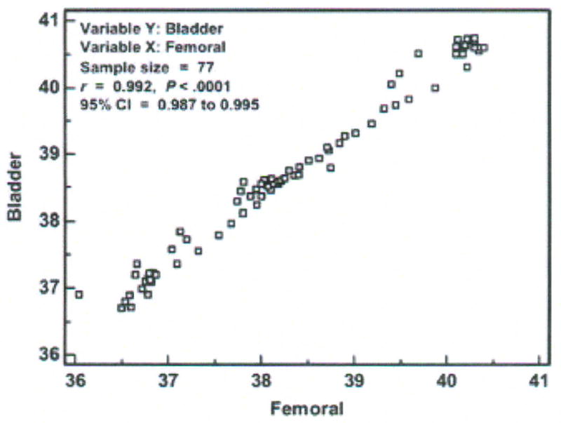
Scatter diagram, correlation coefficient (r), and 95 % confidence interval (CI) of temperatures (degrees Centigrade) measured with the bladder and femoral methods in one critically ill porcine subject (P003). Data points represent averages of 30-minute aggregates.
If one were to imagine a diagonal line at the intersection of each degree of temperature on both axes from 36 to 41°C, the diagonal line (called the line of equality or the line of identity) would be the line on which all data points would fall if there was perfect agreement between methods. Selection of the Info option from a right mouse click on the graph displays the correlation of temperature values measured with the two methods. The Pearson Product-moment correlation for the individual data points was r = .992, with a significance level of p < 0.0001, and 95% confidence interval (CI) for r of .987 to .995. The correlation analysis results tell the investigator that: (1) the temperature value obtained with the bladder method is strongly associated with the temperature value obtained with the femoral method; (2) the probability that this association was due to chance is less than 1 in 10,000; and (3) when these methods are used in another subject like this one and in similar conditions, we can be confident that the r will be between .987 and .995. As mentioned earlier, inferences cannot be made from one subject as is the case here, so (3) above would be applicable in the usual circumstance where there are multiple subjects.
However, the strong correlation between the bladder and femoral temperatures does not tell us about agreement between the methods. Indeed, the scatter diagram shows disagreement. If the methods resulted in perfect agreement, all the paired data points would fall on the diagonal line. We see this is not the case even though the data points fall close to the line of equality. Further analysis is needed to determine both the magnitude and direction of the bias.
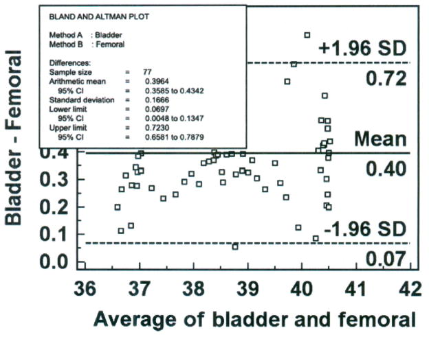
The next step is to construct a Bland-Altman plot as shown in Figure 3. The x-axis represents the average temperature obtained with the bladder and femoral methods across the range of temperatures between 36 and 42°C. The normal temperature of the domestic farm pig is 39°C,17 so in this subject the methods of measurement were compared in conditions of hypothermia, euthermia and hyperthermia, satisfying the design consideration of conditions of measurement. The y-axis represents the difference in temperature measured with the bladder and femoral methods. In this case, the differences vary from 0.05 to 0.86°C; all differences are positive, which means that the bladder method measured temperature higher than the femoral method. Because all the observed differences were greater than zero, there is a systematic bias. In other words, regardless of the temperature value between 36 and 42°C, the difference between methods was positive. Because the difference scores represent the bladder measurement minus the femoral measurement, the bladder method had a positive bias and yielded a higher temperature than that measured simultaneously with the femoral method. While the positive bias for each paired measurement point varied from 0.05 to 0.86°C, across all 77 paired measurements the average difference was 0.40°C (solid horizontal line), the value that would be reported as the bias for this data set.
Figure 3.
Bland-Altman plot of bladder and femoral temperatures (degrees Centigrade), averaged over 30 minutes for each data point with mean (bias) and ± standard deviation (SD) temperature differences for all values, from one porcine critically ill subject (P003).
The dotted horizontal lines represent the 95% confidence limits (limits of agreement). The SD of the difference scores for this data set was 0.167°C (obtained by the Info option from right-clicking the mouse on the Bland-Altman plot). MedCalc computed the upper limit of agreement as 1.96 (2 SD) times 0.167 (SD) plus 0.40 (bias), which yields 0.72°C. Similarly, MedCalc computed the lower limit of agreement by 1.96 (2 SD) times 0.167 (SD) minus 0.40 (bias), yielding 0.07°C. Thus, if the differences between methods were distributed normally, 95% of the differences from the bias in the sample are expected to be between 0.07 and 0.72°C. The confidence limit (0.72 − 0.07°C = 0.65°C) exceeds the a priori criterion of 0.2°C, so the investigator would conclude that the repeatability of the method is unacceptable and, thus, the bladder method is not equivalent to the femoral method. It is noted that 4 of 77 (5%) data points exceed the limits of agreement; three exceed the upper limit and one exceeds the lower limit.
We next examine the Bland-Altman plot to determine if the temperature differences between methods are dependent on the temperature value (the average of the two methods on the x-axis). It appears that the differences are scattered around the bias, with no obvious pattern. The difference is no more likely to be higher or lower at 40.4 than at 36°C (the maximum and minimum temperature values in this data set); thus, calculation of percentage error is not indicated. Nonetheless, percentage error is calculated here to demonstrate the procedure. The numerator is the confidence limit (upper limit of agreement of 0.72°C minus lower limit of agreement of 0.07°C = 0.65°C). The denominator is the mean temperature value of the established method (38.41°C), obtained from the frequency distribution descriptive statistics; unfortunately, descriptive statistics are not an available option in the MedCalc program, and were obtained for this example from SPSS (Version 15.0 for Windows, SPSS Inc., Chicago, IL). The percentage error is 1.7% (0.65 divided by 38.41 multiplied by 100), which validates our conclusion of no obvious proportional pattern from inspection of the Bland-Altman plot.
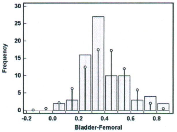
The difference scores were evaluated for a Normal distribution in two ways: (1) Kolmogorov-Smirnov test for Normal distribution and (2) histogram. The Kolmogorov-Smirnov test evaluates the extent of discrepancy between the sample distribution and the Normal distribution (i.e., bell-shaped curve). A p value ≥ 0.05 indicates no significant difference between the two distributions and the conclusion is that the sample distribution is approximately Normal; thus, the sample data can be described by mean ± SD and subjected to parametric statistical tests. A p value < 0.05 indicates a significant difference between the two distributions (i.e., the difference scores are not normally distributed), and the data should not be subjected to parametric testing. In the temperature data set under discussion, p = 0.221 and passes the test for Normal distribution. In MedCalc, the Kolmogorov-Smirnov test can be selected from the Summary Statistics option under the Statistics function.
A histogram was constructed and is shown in Figure 4. The x-axis contains the difference scores between the bladder and femoral methods in increments of 0.1°C. The difference scores vary from 0.05 to 0.86°C as seen in the y-axis of Figure 3. The bars represent the sample difference scores and the superimposed vertical lines represent a Normal distribution. Discrepancy between the sample difference scores and the Normal distribution is seen at all intervals of difference scores. The data set produced no difference scores at intervals of − 0.2 to − 0.05°C; more scores at the intervals of 0.25, 0.35 and 0.75°C; and fewer scores at the intervals of 0.15, 0.45, 0.55, and 0.65°C than would occur if the difference scores were perfectly normally distributed. Nonetheless, the data set difference scores approximately follow the superimposed Normal distribution, and, together with rejection of the hypothesis that there is a significant difference between the two distributions by the Kolmogorov-Smirnov test (p = 0.221), there is evidence of approximately Normal distribution. We can estimate that 95% of the difference scores for other similar subjects measured under similar conditions will fall between 0.07 and 0.72°C (the Bland-Altman limits of agreement).
Figure 4.
Histogram of differences in temperatures (degrees Centigrade) measured with the bladder and femoral methods in one porcine critically ill subject (P003).
The reader will recall that the clinically acceptable bias of 0.5°C was set a priori for these experiments. Given that the difference scores are normally distributed, the precision of the bias can be computed with the 95% CI. This computation requires the standard error of the mean (SEM), in contrast to the SD used to compute the limits of agreement in the Bland-Altman plot. MedCalc automatically computes the CI for bias, using the SEM and the t distribution as bias ± (95% critical value of t times SEM) in the Summary Statistics function. In this data set, the 95% CI for bias is 0.36 to 0.43°C. Therefore, we can be 95% confident that the true bias of the population will fall between 0.36 and 0.43°C. Selection of the Info option by right-clicking the mouse in the Bland-Altman plot displays the bias (Arithmetic mean), the 95% CI for the bias, the SD of the difference score, and the 95% CI for the upper and lower limits of agreement as shown in Figure 5.
Figure 5.
Bland-Altman plot of bladder and femoral temperatures (degrees Centigrade), averaged over 30 minutes for each data point with mean (bias) and ± standard deviation (SD) temperature differences for all values, from one porcine critically ill subject (P003), with quantitative estimates superimposed.
A report of the findings from this data set would include the following information: Mean temperature of 38.41 (± 1.3°C), bias of the bladder method of measurement = 0.40 (95% CI = 0.36, 0.43°C), SD = 0.167°C (95% limits of agreement = 0.07, 0.72°C and their respective 95% CIs), and percentage error = 1.7%. The Bland-Altman plot would be included in a figure.
Procedural Example
A second example is provided with interpretation, but without explanation, to illustrate the steps using the MedCalc software program with the procedure used by the author. In this example, the rectal method of temperature measurement from the same subject is compared with the femoral artery method to determine method agreement. The a priori criteria for bias and precision are 0.5 ± 0.2°C.
Step 1 – Create database in Excel for import into MedCalc (Figure 6)
Figure 6.
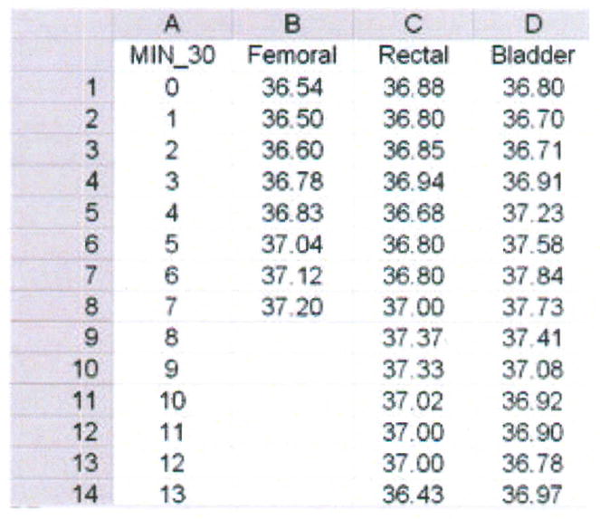
Data base for femoral, rectal and bladder temperatures (degrees Centigrade), averaged over 30 minutes for each data point, from one porcine critically ill subject (P003).
The rows contain the data for each member of the sample. In this case, “member” of the sample constitutes a 30-minute aggregate of temperature measured every second over 43 hours in one subject. The mean temperature at each 30-minute interval for the femoral (established), rectal (test) and bladder (test) methods are displayed respectively in columns B through D. Rows 9 through 14 are blank for the femoral artery data because of missing data.
Step 2 – Display scatter diagram using the Info option (Figure 7)
Figure 7.
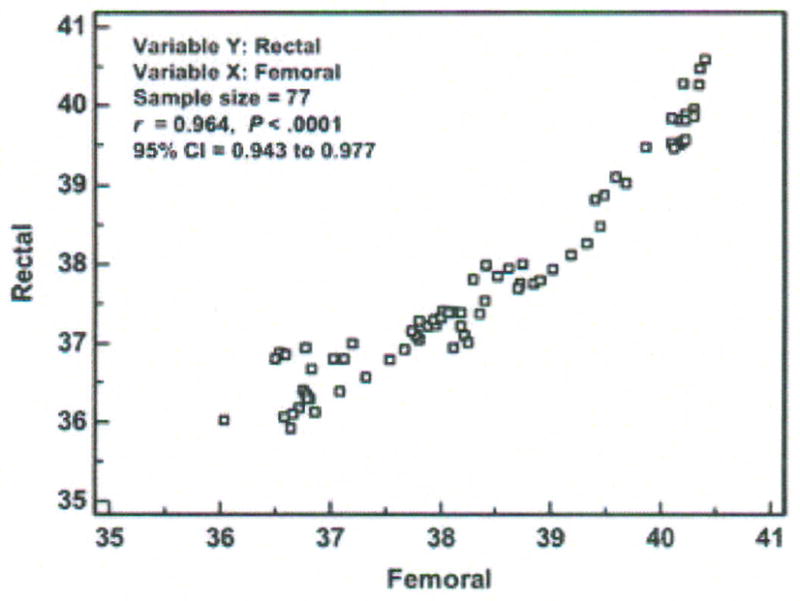
Scatter diagram, correlation coefficient (r), and 95 % confidence interval (CI) of temperatures (degrees Centigrade) measured with the rectal and femoral methods in one critically ill porcine subject (P003). Data points represent averages of 30-minute aggregates.
The data points fall near but not on the line of equality, suggesting there is some degree of disagreement between methods. The correlation coefficient is 0.96 (p < 0.0001; 95% CI = 0.94, 0.98).
Step 3 – Construct Bland-Altman Plot (Figure 8)
Figure 8.
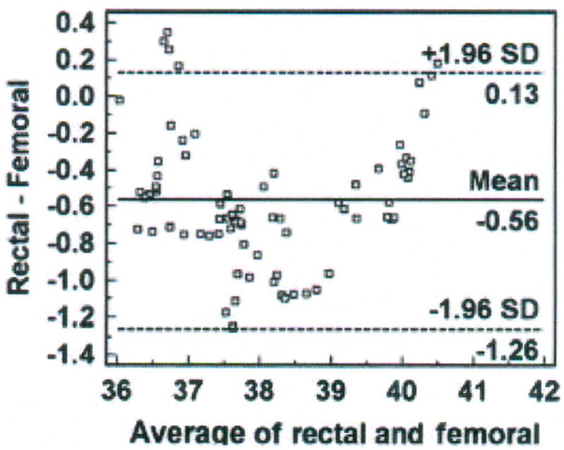
Bland-Altman plot of rectal and femoral temperatures (degrees Centigrade), averaged over 30 minutes for each data point with mean (bias) and ± standard deviation (SD) temperature differences for all values, from one porcine critically ill subject (P003).
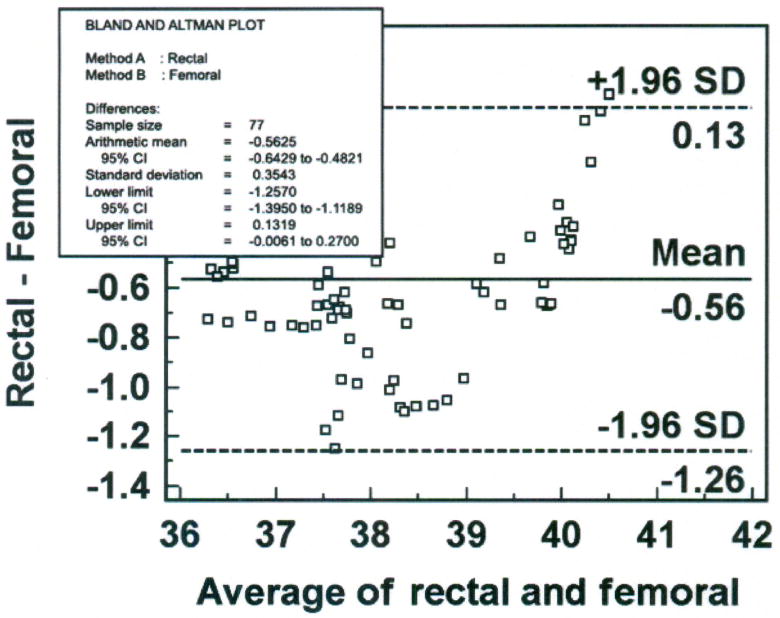
Six percent (5 of 77) of the data points are outliers, and exceed the upper limit of agreement. The bias (SD) of the rectal method is − 0.56 (± 0.35°C), indicating that the rectal method measured lower temperature than the femoral artery method. The plot suggests that differences between the two methods are greater between 37.5 and 39°C than at other temperatures measured. Nonetheless, there is a negative bias for the rectal method, with 70 of the 77 data points falling below zero. Although the differences are skewed, the sample distribution is approximately Normal as indicated by the Kolmogorov-Smirnov test for Normal distribution (p = 0.484). The SEM is 0.04°C.
Step 4 – Compute percentage error
The percentage error is 3.6% (confidence limit of 1.39 divided by mean temperature value of 38.4°C multiplied by 100), over twice as high as the percentage error for the bladder method in the previous example.
Step 5 – Construct histogram of difference scores (Figure 9)
Figure 9.
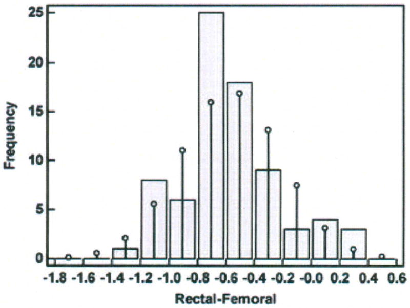
Histogram of differences in temperatures (degrees Centigrade) measured with the rectal and femoral methods in one porcine critically ill subject (P003).
The difference scores are distributed in an approximately Normal pattern around the bias of −0.56°C.
Step 6 – Compute 95% CI for bias and the limits of agreement (Figure 10)
Figure 10.
Bland-Altman plot of rectal and femoral temperatures (degrees Centigrade), averaged over 30 minutes for each data point with mean (bias) and ± standard deviation (SD) temperature differences for all values, from one porcine critically ill subject (P003), with quantitative estimates superimposed.
The 95% CI for the bias is − 0.64 to − 0.48°C, a wider interval than that computed for the bias of the bladder method. The 95% CI is − 0.006 to 0.270 for the upper limit of agreement and −1.40 to − 1.12 for the lower limit of agreement.
Step 7 – Interpret findings against a priori criteria
The mean (± SD) temperature of the femoral artery method was 38.41 (± 1.3°C), compared with 37.84 (± 1.32°C) for the rectal method. The bias of the rectal method was − 0.56°C (95% CI = − 0.64, − 0.48), precision was 0.35 (95% confidence limit = − 1.26, 0.13°C), and percentage error was 3.6%. The bias and precision exceeded the a priori criteria of 0.5 ± 0.2°C; thus, the rectal method cannot be used in lieu of the femoral artery method of temperature measurement for the investigator’s purpose of determining circadian temperature rhythm in critically ill swine.
Summary
The purpose of this paper was to provide information on the design, analysis and interpretation of method-comparison studies to assist clinicians with (1) the evaluation of a new method compared with an established one for measuring a variable of clinical interest and (2) interpretation of method-comparison studies in the literature. Two examples of temperature methods were used. The availability of such software as MedCalc eliminates the need for detailed statistical computation. Even so, for interpretation of the bias and precision statistics, it is advisable to collaborate with a scientist or statistician in the design and conduct of method-comparison studies, particularly when encountering complex data sets and patterns. The reader who wants more information is referred to two excellent, older articles that address method-comparison methodology with the use of blood pressure and arterial blood gas measurement, respectively.18, 19
Acknowledgments
Appreciation is expressed to Nikhil Padhye, PhD; Stanley G. Cron, MSPH; Shannan Hamlin, MSN, RN, ACNP; Gary Gusick, DSN, RN; and Mary Anne Vincent, MS, RN, CCRN, for critique of the manuscript.
Financial Support
This work was partially supported by grant R15-NR04488 from the National Institute of Nursing Research, National Institutes of Health.
References
- 1.Giuliano KK, Scott SS, Elliot S, Giuliano AJ. Temperature measurement in critically ill orally intubated adults: A comparison of pulmonary artery core, tympanic, and oral methods. Crit Care Med. 1999;27:2188–2193. doi: 10.1097/00003246-199910000-00020. [DOI] [PubMed] [Google Scholar]
- 2.Hebbar K, Fortenberry JD, Rogers K, Merritt R, Easley K. Comparison of temporal artery thermometer to standard temperature measurements in pediatric intensive care unit patients. Pediatr Crit Care Med. 2005;6:557–561. doi: 10.1097/01.pcc.0000163671.69197.16. [DOI] [PubMed] [Google Scholar]
- 3.Schuh S, Komar L, Stephens D, Chu L, Read S, Allen U. Comparison of the temporal artery and rectal thermometry in children in the emergency department. Pediatr Emerg Care. 2004;20:736–741. doi: 10.1097/01.pec.0000144915.78124.26. [DOI] [PubMed] [Google Scholar]
- 4.Moran JL, Peter JV, Solomon PJ, et al. Tympanic temperature measurements: Are they reliable in the critically ill? A clinical study of measures of agreement. [Accessed September 4, 2007];Crit Care Med [serial online] 2007 35:155–164. doi: 10.1007/s00134–007–0743–7. Published online June 19, 2007. [DOI] [PubMed] [Google Scholar]
- 5.Lawson L, Bridges EJ, Ballou I, et al. Accuracy and precision of noninvasive temperature measurement in adult intensive care patients. AJCC. 2007;16:485–496. [PubMed] [Google Scholar]
- 6.de Waal EEC, Kalkman CJ, Rex S, Buhre WF. Validation of a new arterial pulse contour-based cardiac output device. Crit Care Med. 2007;35:1904–1909. doi: 10.1097/01.CCM.0000275429.45312.8C. [DOI] [PubMed] [Google Scholar]
- 7.Halvorsen PS, Sokolov A, Cvankarova M, Hol PK, Lundblad R, Tonnessen TI. Continuous cardiac output during off-pump coronary artery bypass surgery: Pulse-contour analyses vs pulmonary artery thermodilution. [Accessed September 4, 2007];Br J Anaesth. 2007 99:484–492. doi: 10.1093/bja/aem199. Published July 24,2007. [DOI] [PubMed] [Google Scholar]
- 8.Lacara T, Domagtoy C, Lickliter D, et al. Comparison of point-of-care and laboratory glucose analysis in critically ill patients. AJCC. 2007;16:336–346. [PubMed] [Google Scholar]
- 9.Hanneman SK, Jesurum-Urbaitis JT, Bickel DR. Comparison of methods of temperature measurement in swine. Lab Anim. 2004;38:297–306. doi: 10.1258/002367704323133682. [DOI] [PubMed] [Google Scholar]
- 10.Mantha S, Roizen MF, Fleisher LA, Thisted R, Foss J. Comparing methods of clinical measurement: Reporting standards for Bland and Altman analysis. Anesth Analg. 2000;90:593–602. doi: 10.1097/00000539-200003000-00018. [DOI] [PubMed] [Google Scholar]
- 11.Molnar Z, Umgelter A, Toth I, et al. Continuous monitoring of ScvO2 by a new fibre-optic technology compared with blood gas oximetry in critically ill patients: a multicentre study. [Accessed September 4, 2007];Intensive Care Med. 2007 doi: 10.1007/s00134–007–0743–7. [DOI] [PubMed] [Google Scholar]
- 12.Altman DG, Bland JM. Measurement in medicine: The analysis of method comparison studies. The Statistician. 1983;32:307–317. [Google Scholar]
- 13.Bland JM, Altman DG. Statistical methods for assessing agreement between two methods of clinical measurement. Lancet. 1986;1:307–310. [PubMed] [Google Scholar]
- 14.Bland M. An Introduction to Medical Statistics. 2. New York, NY: Oxford University Press; 1995. [Google Scholar]
- 15.Critchley LAH, Critchley JAJH. A meta-analysis of studies using bias and precision statistics to compare cardiac output measurement techniques. J Clin Monit Comput. 1999;15:85–91. doi: 10.1023/a:1009982611386. [DOI] [PubMed] [Google Scholar]
- 16.Hanneman SK, Clubb FJ, McKay K, Costas G. Feasibility of a porcine adult intensive care model. Comp Med. 2004;54(1):36–43. [PubMed] [Google Scholar]
- 17.Ingram DL, Mount LE. The effects of food intake and fasting on 24-hourly variations in body temperature in the young pig. Pflugers Arch. 1973;339:299–304. doi: 10.1007/BF00594165. [DOI] [PubMed] [Google Scholar]
- 18.Liehr P, Dedo YL, Torres S, Meininger JC. Assessing agreement between clinical measurement methods. Heart Lung. 1995;24:240–245. doi: 10.1016/s0147-9563(05)80043-3. [DOI] [PubMed] [Google Scholar]
- 19.Szaflarski NL, Slaughter RE. Technology assessment in critical care: Understanding statistical analyses used to assess agreement between methods of clinical measurement. AJCC. 1996;5:207–216. [PubMed] [Google Scholar]


