Whether you’re a seasoned financial analyst or a data-proficient professional, understanding the calculation of investment returns can help assess the profitability and risks of various assets. This post explores three core methods for calculating investment returns: normalized returns, daily returns, and logarithmic daily returns.

The integration of Python within Excel provides a powerful tool for these calculations. Python’s extensive libraries combined with Excel’s widespread use in finance create a potent duo for enhancing analytical capabilities, automating tasks, and ensuring precise, thorough analyses.

To get started, download the exercise file linked below.

To begin, I’ll read the source table into Python in Excel as a DataFrame and set the index to the Date column. This step will simplify many of our visualizations and calculations. We’ll be able to calculate and plot all three stocks simultaneously. While this plot provides the essential raw stock prices, it may be challenging to assess the relative risk and return of each investment.

The first step we’ll take is to plot the normalized returns.

Normalized prices, typically calculated by comparing the price at the initial time (t_0) with the price at a subsequent time (t+1), offer a method to assess price changes over a specified interval. This technique mirrors the calculation of cumulative daily returns, focusing on how prices shift from one trading day to the next.

By examining these differences, we can monitor the percentage changes in asset prices, thereby gaining insights into market trends and the overall performance of investments. This method proves particularly valuable in financial analysis for comparing the performance of various assets over time, irrespective of their initial price levels.

To achieve this with Python, I can simply divide each row by the first row in the dataset:

returns_normed = stocks/stocks.iloc[0]
returns_normed.plot()

One particularly nice feature of having the Date column set as the Index of our DataFrame is the ease with which we can filter for specific date ranges. For example, if I want to plot data starting from March 2020, I can do it like this:

returns_normed['2020-Mar':].plot()

Next, we’ll calculate the daily returns.

This method calculates the ratio of each day’s stock price to the previous day’s price, effectively measuring the day-to-day percentage change in stock prices. Daily returns are useful for understanding short-term price movements and volatility, providing insights into how stock prices fluctuate on a daily basis. This information is essential for traders and analysts who focus on short-term market trends and risk management.

returns_daily = stocks/stocks.shift(1)
returns_daily.plot()

In contrast, our first technique normalized the stock prices by dividing each day’s price by the initial price (the price on the first day of the dataset). This approach tracks the cumulative growth or decline of the stocks over the entire time period.

Normalized returns are valuable for long-term analysis, as they show the overall performance and growth trajectory of the investments relative to their starting point. While daily returns focus on short-term variations, normalized returns provide a broader perspective on the long-term performance of the stocks.

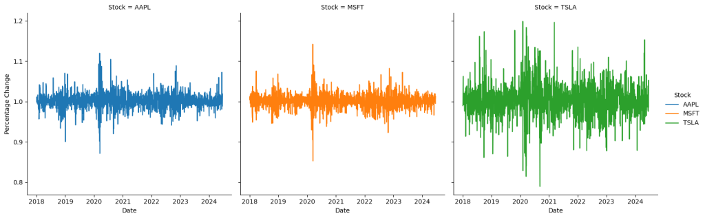
It’s great that daily returns place each stock on the same relative scale to 100, but it makes the plot crowded and hard to read. One solution is to use small multiples. I find this easier to do in Seaborn, but we’ll need to reshape our data first:

returns_daily = returns_daily.reset_index()
melted_df = returns_daily.melt(id_vars='Date', var_name=
'Stock', value_name='Percentage Change')

sns.relplot(data=melted_df, x='Date', y='Percentage Change', row='Stock', kind='line', hue='Stock')

When you take the daily returns of an investment and calculate their cumulative product, you get something familiar: normalized returns! This process essentially tracks the growth of the investment over time, starting from a baseline value, often set to 1.

returns_daily.cumprod().plot()

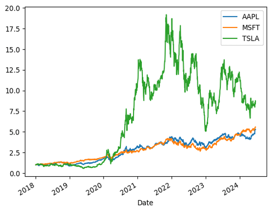
By continuously multiplying each day’s return by the product of all previous returns, you can see how the investment has grown or shrunk over the period. This normalized return series provides a clear picture of the investment’s performance, showing how much a $1 investment at the beginning would be worth at any given point in time, reflecting all the daily fluctuations.

Lastly, we can calculate the log returns. These are the natural logarithm of the ratio of consecutive prices. Log returns are useful because they are time additive, meaning the log return over multiple periods is the sum of the individual period returns. This property simplifies the aggregation of returns over different intervals.

Additionally, log returns often follow a normal distribution, making them easier to analyze statistically. Plotting log returns provides a clear view of day-to-day volatility and performance, helping to identify patterns and trends in the data.

log_returns = np.log(stocks/stocks.shift(1))
log_returns.plot()

We could similarly break these log returns into smaller intervals to make them easier to view. However, instead, let’s use a bit of mathematical magic to convert these back to daily returns.

By taking the cumulative sum of the log returns and then applying the exponential function, we effectively reverse the logarithm transformation. This gives us a continuous product of the returns, similar to how we initially calculated normalized returns.

log_returns.cumsum().apply(np.exp).plot()

What questions do you have about calculating investment returns with Python in Excel? Let me know in the comments.

If you’re looking to get your team started with Python for financial data analytics, feel free to get in touch:

The post Python in Excel: How to calculate investment returns first appeared on Stringfest Analytics.