Discriminative Subspace Clustering Vasileios Zografos∗1 , Liam Ellis†1 , and Rudolf Mester‡1 2 1 2 CVL, Dept. of Electrical Engineering, Linköping University, Linköping, Sweden VSI Lab, Computer Science Department, Goethe University, Frankfurt, Germany Abstract lar subspace. For this reason, in the last few years a large number of scientific publications in computer vision and machine learning literature have emerged proposing a wide range of sophisticated solutions to the subspace clustering problem. Notable examples are the SCC method [2], where the authors utilize the normalized volume (spectral curvature) of the (d+1)-dimensional simplex formed by random (d+2) points; The SC approach by [3], which looks at the cosine angle between pairs of points for clustering them together, and as such is suited for linear-only subspaces; The SLBF method [4], which defines a subspace at every point, supported by its local neighborhood, with the neighborhood size determined automatically; The SSC method [5], which describes every point by a set of sparse linear combinations of points from the same subspace. The sparsity information is then used as a point clustering affinity. More recent examples are the LRR method by [6], that tries to recover a low-rank representation of the data points, and its improvement LLRR [7], which is able to handle the effects of unobserved (“hidden”) data by solving a convex minimization problem. Finally, we have the two algebraic methods SSQP [8] and LSR [9]. The former works on the premise that every data point is a regularized linear combination of few other points, and a quadratic programming approach is used to recover such configurations. LSR is a fast method which takes advantage of the data sample correlation and groups points that have high correlation together. We present a novel method for clustering data drawn from a union of arbitrary dimensional subspaces, called Discriminative Subspace Clustering (DiSC). DiSC solves the subspace clustering problem by using a quadratic classifier trained from unlabeled data (clustering by classification). We generate labels by exploiting the locality of points from the same subspace and a basic affinity criterion. A number of classifiers are then diversely trained from different partitions of the data, and their results are combined together in an ensemble, in order to obtain the final clustering result. We have tested our method with 4 challenging datasets and compared against 8 state-of-the-art methods from literature. Our results show that DiSC is a very strong performer in both accuracy and robustness, and also of low computational complexity. 1. Introduction It is well known that various tasks in computer vision, such as motion segmentation; face clustering under varying illumination; handwritten character recognition; image segmentation and compression; and feature selection, may be solved as low-dimensional linear subspace clustering problems (see [1]). Since in most natural data the total variance is contained in a small number of principal axes, even if the measured data is high-dimensional, its intrinsic dimensionality is usually much lower. Furthermore, it is reasonable to model data which comes from different classes as lying in a union of linear subspaces, rather than in a single subspace. Therefore, the problem of high-dimensional data segmentation, simplifies to one of lower-dimensional subspace clustering. That is, recovering the appropriate linear subspaces and the membership of each data point to a particu∗ zografos@isy.liu.se We present a novel method for the solution of the subspace clustering problem, which follows the machine learning principle of Discriminative Clustering, that is, solving an unsupervised learning problem by means of a classifier or put more simply “clustering by classification”. Our method is called Discriminative Subspace Clustering (DiSC) and is fundamentally different from the generative, often algebraic methods that one encounters in subspace clustering literature. 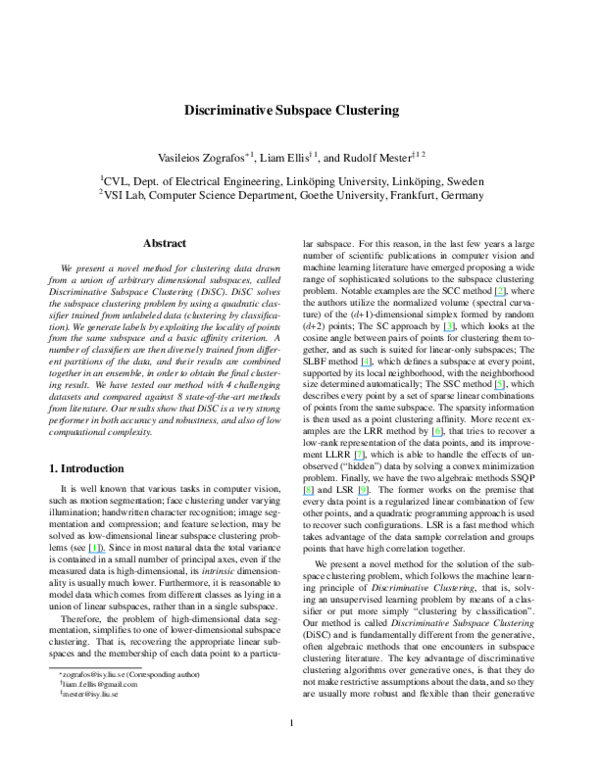The key advantage of discriminative clustering algorithms over generative ones, is that they do not make restrictive assumptions about the data, and so they are usually more robust and flexible than their generative (Corresponding author) † liam.f.ellis@gmail.com ‡ mester@isy.liu.se 1 Figure 1. The DiSC method overview. First we extract partial labels from unlabeled data. These labels are used to train a classifier, which in turn separates the data into different classes, thereby solving the subspace clustering problem. counterparts. Furthermore, obtaining a generative model can often be difficult in many application domains. Conversely in discriminative algorithms, performance can be affected by incomplete and noisy training data. However as we will show, this potential problem can be minimized by the information leveraging abilities of ensemble clustering. DiSC exploits three very simple observations: First and foremost is that two subspaces in general configurations (i.e. non-coincidental intersection) can be optimally separated by a quadratic classifier; Second is the locality principle. Namely that very often a point lies in close proximity to a small number of points from the same subspace; And third, that by combining together the results of multiple, diversely-trained classifiers (ensemble), we can obtain an overall improved result. The first requires the provision of labels. The second provides a set of weak (incomplete and noisy) labels, and the third generates a final, robust result from an ensemble of diverse clusterings. Our contribution with this paper is the combination of these three basic observations inside a workable discriminative clustering framework and the production a novel method for the accurate and robust solution of the subspace clustering problem. We have tested our method on a number of real and synthetic datasets and against state-of-theart approaches from literature. The experiments show that DiSC compares very favorably against the other methods. In addition, it is stable to parameter settings and has low complexity as a function of the number of subspaces, the number of points and the number of ambient dimensions. 2. Our approach We may define a subspace of dimensionality d<D as:  L = x ∈ RD : x = µ + Uy , (1) with µ∈RD an arbitrary point1 on the subspace, U∈RD×d is some basis for the subspace and y∈Rd are the coordinates  N of x in the basis U. Given a set of N points xj ∈ RD j=1 1 If µ = 0 then L is linear subspace, otherwise it is an affine subspace SK that is drawn from a union of K subspaces i=1 Li , the objective of subspace clustering is to recover the number of subspaces K, their dimensions di , their bases Ui , the points µi and the membership of the data points x to each subspace. However, in practice it is sufficient to recover only the membership of points to subspaces, since given a correct membership (clustering) it is straightforward to find the remaining parameters per subspace afterwards, using for example PCA. Therefore the majority of methods from the literature, including ours, only solve the membership sub-problem, given some general information, such as the number K of subspaces and their maximum intrinsic dimensionality d=max(di ). Our approach, DiSC, involves formulating and solving the subspace clustering problem inside a discriminative clustering framework, without having to rely on a strong generative model a-priori. An overview of DiSC can be seen in Fig. 1. We first label a subset of the unlabeled data. These labels are used to train a classifier and finally the classifier gives a solution to the problem. It is important to provide the classifier with consistent and representative data. By consistent we mean data samples belonging to the same subspace, having the same labels. By representative we mean data that is sampled regularly and sufficiently, so that no populated region of the subspaces is neglected. Such labeled data is obtained from an unlabeled set, using the principle of locality (or “common fate”) in the data points, and a subspace affinity criterion (see Fig. 2 and 3). Of course, due to the unsupervised nature of the data inherent in any clustering problem, we cannot guarantee that the consistency and representativeness requirements will be fulfilled exactly. As a result, the classifier will be a weakly trained one, and as such, it may not be able to solve the subspace clustering problem adequately in every case. In order to improve robustness, we leverage multiple, diverselytrained classifiers and combine their results in an ensemble. Diversity in the classifiers is achieved by two means: random projections and randomized local sampling. With random projections, we project the data into a lower dimensional ambient space using random projection Figure 2. Generating labels from unlabeled subspace data. First we create a small set of random, local clusters. The points in each cluster most likely lie on the same subspace. We then merge these clusters to obtain the training data for the classifier. matrices. This serves a twofold purpose. First it improves the clustering problem by essentially discarding redundant dimensions in the data and second, it provides each classifier with slightly different “views” of the same data. The randomized local sampling on the other hand, improves the ensemble by bootstrap aggregating (or bagging). That is, generating multiple training sets by random sampling with replacement. Once a diverse ensemble of classifier outputs has been produced, we can solve an ensemble clustering problem and obtain a more accurate and robust result than that of a single, weakly-trained classifier. The main algorithm of the DiSC method is presented in Algorithm 1, while its constituent parts are explained in more details next. very small r will increase the dimensionality of the intersection between the subspaces. Given the fact that the intersection is the most problematic region to cluster our aim is to choose r large enough so that the dimensionality of the intersection between subspaces is minimized. Inspired by [3] we chose the projection dimension r = K · max (di ) + 1, i = 1, . . . , K (3) where K is the number of subspaces and di are their intrinsic dimensions. (2) Randomized local sampling Following the random projection, in order to introduce additional ensemble diversity, robustness to noise and avoid overfitting, we select subsets of training data from the union of subspaces by randomized local sampling. The first step of this technique involves generating a number Q<<N of random local clusters consisting of P points each. Random local clusters are formed by initially sampling Q random points from the subspace union, and then forming the clusters around each of these points and their (P -1)-nearest neighbors in the ambient Euclidean distance (see Fig. 2). This is an approach used in many subspace methods and exploits the observation that points on the same subspace generally lie in close proximity to (at least a few) other points from the same subspace. For small neighborhoods, we have a high likelihood of obtaining local clusters which contain points from the same subspace. This likelihood generally decreases for points near the subspace intersection, which is why it is particularly useful to minimize the dimensionality of the intersection in the first place. where X is the original data matrix with N observations in RD . Provided that the new dimensions r are of appropriate size then according to [10] there exists a map which preserves the metric structure of the data introducing only small bounded distortions. Nevertheless, an overly large r will include unnecessary dimensions of noise, whereas a From local to global: Merging The next step involves merging the Q local clusters into K clusters, where K is the number of subspaces. In that way, the classifier will obtain a more representative, “global view” of the data, while at the same time maintaining the consistency in the samples from the previous step. The merging is carried out using spectral clustering [11] with 2.1. Generating labels from unlabeled data Random data projection A typical first step in many subspace segmentation methods is dimensionality reduction in order to simplify the clustering problem, especially if the ambient dimensionality of the data is very large. A common such technique is PCA, which despite being expensive to compute, is deterministic and unique and an optimal mean square projection. In our case however, we are not only interested in the dimensionality reduction but also in introducing diversity in classifiers, by obtaining similar but slightly different views of the training data. Instead of carrying out PCA, we perform a different dimensionality reduction projection to Rr √ for each classifier, using a Gaussian (0, 1/ r) distributed random projection matrix R[r×D] such that e = RX, X the basic model can be extended further to incorporate additional information about the subspace data. Assume that we have training data xi ∈ RD that lives in a union of subspaces Li , and classes ωi , corresponding to each subspace. We also have a new observation z ∈ RD for which we wish to make a classification decision. A reasonable decision rule is to assign z to the class with the highest posterior probability P (ωi |z) > P (ωj |z), ∀i 6= j. Figure 3. Mutual projection affinity between two clusters. For each cluster we fit a local subspace and project the points of the other cluster to the subspace. We then calculate the average projection residual and use an exponential kernel to create the affinity. This affinity is very effective and more robust than algebraic affinities. the aid of a subspace-based affinity. Here, since we need to merge clusters together, we define the “mutual projection distance” between two clusters Cq and Cs as: E(q, s) = 1 2 q δ (xq , Ls ) + 1 2 q δ (xs , Lq ), Since the vectors xi are restricted to live on the subspaces, the observation model must necessarily integrate a measurement error term, otherwise the model cannot explain arbitrary data z ∈ RD . Thus we consider an additive measurement error term ν z = x + ν. (7) A reasonable assumption about ν is that it is zero-mean isotropic and Gaussian distributed
p(ν) = cν exp −1/2ν T [σν2 I]−1 ν , (8) with cν a normalization constant and σν2 the scale of the noise. Then the first two moments of xi are: (4) where δ (xq , Ls ) is the mean squared orthogonal distances of points x ∈ Cq , to the subspace Ls defined by cluster Cs (see Fig. 3). It is obvious then that we need at least P ≥ d + 1 points in each cluster. The clusters are allowed to overlap, but duplicate points are removed before being passed into the classifier. The distance in (4) is turned into an affinity by using the exponential kernel as (6) E[xi ] Cov[xi ] = µi , = Ui Cov[yi ] UTi , (9) where y is defined in (1). Since Cov[xi ] has rank di < D, we avoid writing down the expression for p(x|ωi ) and instead point out that for any two uncorrelated random variables x, ν we have: E[xi + ν] Cov[xi + ν] = E[xi ] + E[ν], = Cov[xi ] + Cov[ν]. (10) From (7), (10) we obtain: A(q, s) = exp (−E(q, s)/α) , (5) where α is the kernel width, and is related to the amount of noise in the data. The affinity in (5) is based on a geometric residual and because of that it is more robust to noise than algebraic residuals, it can deal with mixtures of subspaces of different dimensionalities, and scales well with an increase in intrinsic and ambient dimensions. The merging step is summarized in Algorithm 2. The number of local clusters we sample is always fixed at Q=0.1N and with P =d+3 points. In the end, we obtain a representative set of points with consistent labels that come from each subspace (see Fig. 2), which forms the classifier training set. 2.2. The quadratic classifier for subspace data The quadratic classifier is known to be a minimum Euclidean distance classifier for data that is modeled using projections onto subspaces [12]. Here we examine the classification problem from a statistical viewpoint and show how E[z|ωi ] Czi = Cov[zi ] = µi , = Cov[xi ] + σν2 I. (11) Since I is full rank, Czi is also full rank. From the first two moments of zi we can define a parametric model of p(z|ωi ) as:   T exp − 21 (z − µi ) C−1 zi (z − µi ) . (12) p(z|ωi ) = 0.5 D/2 (2π) |Czi | We may now define a parametric form of the discriminant boundary between two classes ω1 , ω2 , and assuming that the class priors have simple forms (i.e. the class frequencies), as:   1/2 T |Cz2 | exp − 21 (z − µ1 ) C−1 z1 (z − µ1 ) n  = 2,  T 1/2 n1 |C | exp − 1 (z − µ ) C−1 z (z − µ ) z1 2 2 2 2 (13) where n1 , n2 are the sizes of the training sets in ω1 , ω2 respectively. By taking the logarithm of (13) and some rearrangement of terms we obtain the quadratic form z T Az + bT z + c = 0, with (14) −1 A =C−1 z1 − Cz2 ,
−1 b =2 µ1 C−1 z1 − µ2 Cz2 , T −1 T c =µ2 C−1 z2 µ2 − µ1 Cz1 µ1 + log (|Cz2 |) − log (|Cz1 |) + 2 (log(n2 ) − log(n1 )) . We can see that (14) determines a second order surface, which is defined by the Mahalanobis distance induced by each training set. In practice, we may simplify the calculation of Czi and avoid the expensive subspace fitting step necessary for recovering Cov[xi ], by estimating: P x, µi ≈ n1i Pi (15) (xi − µi )(xi − µi )T . Cov[xi ] ≈ ni1−1 Then from (11) Czi = Cov[xi ] + ξ 2 I (16) where ξ is a regularization coefficient s.t. ξ ≥ λd+1 with λd+1 being the d + 1 largest eigen-value of Cov[x˜i ]. From the above formulation, and as a direct result of the Gaussian assumption, the quadratic classifier is a minimum Mahalanobis distance classifier. Note that although the quadratic classifier is a generative approach, we are only interested in its discriminative boundaries and we are not using the fitted Gaussian models explicitly. In principle, other pure discriminative classifiers may be used here instead. 2.3. Weighted ensemble clustering After the application of the multiple, weakly trained classifiers we have obtained a number of approximate solutions to the subspace segmentation problem. That is, the set M of clusterings {Ym }m=1 resulting from the classifiers are highly correlated but also exhibit some diversity. Our aim is to now combine these intermediate results for improving the final clustering. Note that because the classifiers have been trained from different subsets and projections of the data, they might not assign identical labels to the same clusters (label permutation). As such, the classifiers cannot be combined directly in a voting scheme or a boosting configuration. However, since a clustering is not affected by the semantics of the labels, what we can do instead is to combine the classifier outputs into a cluster ensemble. For this purpose we have adapted the graph partitioning (HBGF) algorithm by [13]. HBGF combines both the pairwise information between the points and the clustering information from the ensembles as the vertices of a bipartite graph. The edges of the graph specify the point-tocluster memberships. Then the cluster ensemble solution is a min-cut through the set of points. Conceptually, this can be thought of as the volume of the graph encoding how often points end up together. Cutting the graph equates to finding groups of points with high probability of belonging together. M Given an ensemble C={Ym }m=1 of M clusterings with K classes, HBGF creates a “connectivity matrix” Z with N rows corresponding to the points and M · K columns corresponding to the clusterings. Each row of Z is populated in a block-wise fashion as Z(j, Bm ) = 1(j, i, m), j = 1, ..., N (17) with 1(j, i, m) being an indicator function that takes the value 1 if point j has label i in clustering Ym , and 0 otherwise. Bm is the K-sized row block defined as Bm = Z(:, 1 + K(m − 1) : Km). (18) We have made two modifications to the original HBGF algorithm. First we enhance the bipartite graph by including some subspace quality information in the form of the edge weights: ! K p X δ(xi , Li )/α , (19) wm = exp − i=1 with xi being all the points in clustering Ym that have the class label i. Li is the subspace fitted to those points. The function δ() is defined similarly to that in (4) and α is the same parameter to the one used in (5). The weights are applied to each normalized row of Z as: b Bm ) = PZ(:, Bm ) wm . Z(:, m Z(:, Bm ) (20) This has the effect of increasing the edge strength of clusterings with low point-to-subspace projection error, while suppressing edges of clusterings with large errors. The second modification is that the actual graph cut is now carried out with spectral clustering, by creating the bZ b T )β . Spectral clustering has been affinity matrix AZ =(Z chosen because it is much faster and more accurate than the agglomerative clustering initially employed by [13]. Following [11], the optimal value of the β parameter is automatically chosen so as to minimize the overall cluster distortion ∆. The weighted ensemble clustering algorithm is given in Algorithm 3, with a fixed number of ensembles M =50. We note here that the ensemble clustering (including spectral clustering) is also a discriminative step that fits very well into the whole discriminative spirit of the DiSC method. 3. Experiments We now present the results from our comparative experiments on real and synthetic datasets. For all experiments Figure 4. Computational speed experiments for all methods on synthetic data. Left, as a function of sample size. Middle as a function of ambient dimensionality and right as a function of the number of subspaces. The DiSC method is shown in bold. Figure 5. Sensitivity analysis of the important parameters in DiSC, tested on the Hopkins155 dataset over 10 runs. From left-to-right, the number of clusters C, the number of ensembles M , the number of points per cluster P and finally the kernel regularisation parameter α. Algorithm 1 Complete DiSC method Input: Data matrix X[D×N ] , # subspaces K, dim. d Output: N ×1 label vector Y of K classes For each m = 1 : M Random data projection to RKd+1 using (2) Random local sampling of C clusters Merge C local clusters using Algorithm 2 Train quadratic classifier using (16) and (14) Apply classifier to data and obtain clustering Ym Append Ym to ensemble C Ensemble clustering of C using Algorithm 3 to obtain Y Algorithm 3 Weighted ensemble clustering Input: Ensemble C , # subspaces K, α Output: N ×1 label vector Y of K classes b according to (20) Compute matrix Z Distortion ∆ = ∞ For each β = 2 : 8 bZ b T )β AZ = (Z Do spectral clustering on AZ as in [11] with K clusters Obtain result Yβ and clustering distortion ∆β If ∆β < ∆ then ∆ = ∆β and Y = Yβ Algorithm 2 Merging of local clusters Input: Q point clusters, # subspaces K, dimension d, α Output: Q×1 label vector YQ of K classes Fit a subspace L of dim. d to each cluster C using PCA For each q = 1 : Q For each s = 1 : Q Calculate E(q, s) using Cq ,Ls and Cs ,Lq from (4) Calculate A(q, s) using E(q, s) from (5) Do spectral clustering on A as in [11] with K clusters Obtain result YQ which is a standard measure of clustering performance. All tested methods were used with fixed parameters per dataset. When authors provided parameter settings we used those, otherwise we made our best effort to tune them ourselves. SC, SBLF, and SCC required no tuning. DiSC has a single tuning parameter, α from (5). It was kept fixed to α=0.01 for all datasets, except for the MNIST dataset where it was set to α=1 due to the large amount of noise. The first dataset is the Hopkins155 [14], which consists of 155+4 sequences of point trajectories in 2-5 rigidly moving objects. There are approximately 200 points and 30-40 frames in each sequence. Subspace clustering of the motion trajectories amounts to motion segmentation. Each algorithm was given the number of moving objects K and the we have calculated the segmentation error Error = # of missegmented points/N · 100%, (21) intrinsic dimension d=4. The results are shown in Table 1. We can see that DiSC has the lowest segmentation error. Next is the Extended Yale B dataset [15], which contains face images of 28 individuals from 9 poses and under 64 illuminations. We experimented with the illumination subset, since such images are known to live in a low-dimensional subspace. Subspace clustering here amounts to face clustering under illumination variations. All images were rescaled to 160×120 and projected to RKd+1 using PCA. The intrinsic dimensionality was set to d=5 and each subspace contained 64 points. We tested K=2,...,9 by randomly choosing K faces from the 28. We could not go beyond 9 faces since methods such as SSC and SSQP became very slow. We run 100 random tests for each K and the averaged results are shown in Fig. 6. The Extended Yale B has very little noise which is apparent in the initial good performance for all methods. Beyond 5 objects however, accuracy degrades considerably in some approaches. SSC performs the best up to 9 objects, with SLBF and DiSC following closely, with an error of under 1%. The last real image dataset is the MNIST dataset [16] which contains binary images of 10 handwritten digits. The images for each digit live approximately in a subspace of d=3. Because they are handwritten digits, there is a lot of noise present in the dataset. We have used the Test-set of MNIST with 10,000 images of 28×28 pixels. We randomly sampled 200 images from each digit (i.e. points on each subspace) and projected them in R20 . We experimented with random K=2,...,5 digits (subspaces) and again the upper limit was determined by the slow SSC and SSQP. The results after 100 runs for each K are summarized in Fig. 7. We can see that for all methods the segmentation errors are much higher now than before, due to the increased noise. For K=2, LSR is the best performer followed by SSC and DiSC. However as soon as K increases, DiSC becomes the method with the lowest error. Next, we have generated a low-noise, synthetic dataset with random points on subspaces. This set was designed for “torture-testing” each method for robustness to specific geometric configurations of the subspaces and not the noise in the measurements. Tests like this are generally difficult to set up with real data, since datasets such as Hopkins155 and Extended Yale B exhibit low geometric complexity. There are 7 subsets (“difficulty levels”) in the dataset, each adding an extra degree of complexity. For all levels, we have run 100 random tests, each with fixed noise of σ=0.01, random ambient D, random intrinsic d=[1,...,10], random subspaces K=[2,...,5] and random [50,...,150] points per subspace. The 7 levels were constructed as follows: Level 1 (easiest): non-intersecting linear subspaces, D≥Kmax(di )+1, all subspaces of equal dimensions, points drawn from unimodal Gaussian distributions and the intrinsic dimension passed to the algorithms d=di ; Level 2: intersecting sub- Figure 6. Results from the Extended Yale B dataset for up to 9 faces at 64 samples each. The DiSC method is shown in bold. spaces; Level 3: d≥di . This simulates fitting to degenerate subspaces; Level 4: Subspaces of different dimensions. This simulates mixtures of subspaces; Level 5: affine subspaces; Level 6: points drawn from bimodal Gaussian distributions instead (i.e. disconnected point clusters); Level 7: the most difficult, with ambient D=max(di )+1, which does not allow for any dimensionality reduction and the lower bound for the subspace intersection dimensionality is maximal. The results for all levels are illustrated in Fig. 8. We see that only SLBF and DiSC manage to do well for the majority of this dataset. All other methods fail when we allow for degeneracies and subspace mixtures. Note that there is no significant change from using linear to affine subspaces. SLBF fails when at level 6 when we introduce multi-modal point clusters. This is due to the method’s “furthest insertion” sampling scheme that is prone to completely disregarding some clusters. Our method is robust to disconnected clusters even though the classifier is using the unimodal Gaussian assumption. Where we expect our method to deteriorate in performance, is in cases where there is very limited and sparse data on the subspaces, and as a result the locality assumption in the points will not hold. We have also run a limited set of computational speed experiments. Each method has been executed 10 times on synthetic data and on the same computer, and the averaged results are illustrated in in Fig. 4. We see that while DiSC is not the fastest method, it is of low complexity as a function of points N and number of subspaces K, and of almost constant complexity as a function of the ambient dimensions D. Finally, we show some analysis of the sensitivity in the DiSC parameters. Each test was executed 10 times on the Hopkins155 dataset and the graphs of the parameter vs segmentation error (y-axis) are shown in Fig. 5. The most sensitive parameter, as expected, is the kernel parameter α from (5). However, in general a small value usually yields good results, which is why it has been kept fixed for the majority of tested datasets. SC [3] SLBF [4] SCC [2] SSC [5] LRR [6] LLRR [7] SSQP [8] LSR [9] DiSC 1.36% 1.45% 4.119% (0.241) 1.47% 1.64% 1.40% (0.051) 1.49% 3.32% 1.25% (0.025) Table 1. Segmentation results from the Hopkins155 dataset. All numbers show the segmentation error rate (21) averaged over the 159 sequences. Numbers in brackets show the variance (over 100 different runs) for the stochastic methods. the classifiers and discriminant boundaries. Also of interest is the adaptation and application of DiSC to multi-manifold clustering problems. Acknowledgements We would like to thank Klas Norderg, Reiner Lenz and Michael Felsberg for the helpful discussions. This research has received funding from the EC’s 7th Framework Programme (FP7/2007-2013), grant agreement 247947 (GARNICS); from the Swedish Research Council through a grant for the project Extended Target Tracking (within the Linnaeus environment CADICS) and by ELLIIT, the Strategic Area for ICT research, funded by the Swedish Government. Figure 7. Results from the MNIST dataset for up to 5 random digits at 200 samples each. The DiSC method is shown in bold. References [1] R. Vidal, “Subspace clustering,” IEEE Signal Processing Magazine, vol. 28, no. 3, pp. 52–68, March 2011. 1 [2] G. Chen and G. Lerman, “Spectral curvature clustering (SCC),” IJCV, vol. 81, no. 3, pp. 317–330, 2009. 1, 8 [3] F. Lauer and C. Schnörr, “Spectral clustering of linear subspaces for motion segmentation,” in ICCV, 2009. 1, 3, 8 [4] T. Zhang, A. Szlam, Y. Wang, and G. Lerman, “Hybrid linear modeling via local best-fit flats,” IJCV, vol. 100, pp. 217–240, 2012. 1, 8 [5] E. Elhamifar and R. Vidal, “Sparse Subspace Clustering,” in CVPR, 2009. 1, 8 [6] G. Liu, Z. Lin, and Y. Yu, “Robust subspace segmentation by lowrank representation,” in ICML, 2010. 1, 8 Figure 8. Results from the synthetic dataset for the 7 complexity levels. The DiSC method is shown in bold. 4. Conclusion We have presented a novel method for segmenting data drawn from a union of subspaces. Our method, DiSC, solves the subspace clustering problem by using a classifier trained from unlabeled data. We have used the quadratic classifier, which is an optimal minimum Mahalanobis distance classifier for subspace data. We generate training labels by exploiting the locality of points lying on the same subspace and a basic subspace affinity criterion. We diversely train a number of classifiers and combine their outputs in an ensemble to obtain the final clustering solution. Our experiments have shown that our method performs very well compared to the state-of-the-art, is of low complexity and it is robust to complicated geometric configurations of the subspaces. Our future work will be to extend the DiSC algorithm into an online approach, capable of predicting the labels of sequential data and incrementally updating [7] G. Liu and S. Yan, “Latent low-rank representation for subspace segmentation and feature extraction,” in ICCV, 2011. 1, 8 [8] S. Wang, X. Yuan, T. Yao, S. Yan, and J. Shen, “Efficient subspace segmentation via quadratic programming,” in AAAI, 2011, pp. 519– 524. 1, 8 [9] C.-Y. Lu, H. Min, Z.-Q. Zhao, L. Zhu, D.-S. Huang, and S. Yan, “Robust and efficient subspace segmentation via least square regression,” in ECCV, 2012, pp. 347–360. 1, 8 [10] W. B. Johnson and J.Lindenstrauss, “Extensions of Lipschitz mappings into a Hilbert space,” in Conference in Modern Analysis and Probability, vol. 26, 1984, pp. 189–206. 3 [11] A. Y. Ng, M. I. Jordan, and Y. Weiss, “On spectral clustering: Analysis and an algorithm,” in NIPS, 2001, pp. 849–856. 3, 5, 6 [12] E. Oja, Subspace methods of pattern recognition. Research Studies Press, 1983. 4 [13] X. Z. Fern and C. E. Brodley, “Solving cluster ensemble problems by bipartite graph partitioning,” in ICML, 2004. 5 [14] P. Tron and R. Vidal, “A Benchmark for the Comparison of 3-D Motion Segmentation Algorithms,” in CVPR, 2007. 6 [15] A. S. Georghiades, P. Belhumeur, and D. J. Kriegman, “From few to many: Illumination cone models for face recognition under variable lighting and pose,” IEEE PAMI, vol. 23, no. 6, pp. 643–660, 2001. 7 [16] Y. Lecun, L. Bottou, Y. Bengio, and P. Haffner, “Gradient-based learning applied to document recognition,” Proc. of the IEEE, vol. 86, no. 11, pp. 2278 –2324, 1998. 7