Associative Self-organizing Map

0 30 Associative Self-Organizing Map Magnus Johnsson1, Max Martinsson1 , David Gil2 and Germund Hesslow3 2 Computing 1 Lund University Cognitive Science Technology and Data Processing, University of Alicante 3 Department of Experimental Medical Science, Lund 1,3 Sweden 2 Spain 1. Introduction There is not enough genetic information to specify the connectivity of the brain in detail (Miikkulainen et al., 2005). The total number of neurons in the neocortex of an adult human brain is estimated to be about 28 billion and the number of connections (synapses) between them and to other cells in the brain to more than 100 trillion (Mountcastle, 1997). In comparison, the human genome only contains about 3 billion base pairs (Consortium, 2004). Thus a reasonable view is that the cortex is not directly specified genetically but constructed by input-driven self-organization (Miikkulainen et al., 2005). The self-organizing process works by using sensory input to adjust the networks organization instead of specifying all connections in advance. The form of self-organization that seems to be active in the cortex gives rise to a special property called topological mapping. This means that the neurons that are activated for similar sensory inputs are found close to each other. The properties self-organization and topology preservation are caught in the Self-Organizing Map (SOM) (Kohonen, 1988), which shares many features with brain maps (Kohonen, 1990). However, the cortex consists of many brain maps and different parts of the cortex obviously interact. For example, different sensory modalities interact with each other. A dramatic illustration of this can be seen in the McGurk-MacDonald effect. If you hear a person making the sound /ba/ but the sound is superimposed on a video recording on which you do not see the lips closing, you may hear the sound /da/ instead (McGurk & MacDonald, 1976). The neural mechanisms underlying such interaction between different sensory modalities are not known but recent evidence suggests that different primary sensory cortical areas can influence each other. Interaction between sensory modalities may also be important for internal simulation of perceptions. An idea that has been gaining popularity in cognitive science in recent years is that higher organisms are capable of simulating perception. In essence, this means that the perceptual processes normally elicited by some ancillary input can be mimicked by the brain (Hesslow, 2002). There is now a large body of evidence supporting this contention. For instance, several neuroimaging experiments have demonstrated that activity in visual cortex when a subject imagines a visual stimulus resembles the activity elicited by a corresponding ancillary stimulus (for a review of this evidence see e.g. (Kosslyn et al., 2001); for a somewhat different interpretation, see (Bartolomeo, 2002). 2 604 Self- Organising NewAlgorithm Achievements Self Organizing Maps ApplicationsMaps, and Novel Design A critical question here is how simulated perceptual activity might be elicited. One possibility is that signals arising in the frontal lobe in anticipation of consequences of incipient actions are sent back to sensory areas (Hesslow, 2002). Another possibility is that perceptual activity in one sensory area can influence activity in another. Inspired by these findings we suggest that in a multimodal perceptual model, the subsystems of different sensory modalities should co-develop and be associated with each other. This means that suitable activity in some modalities that for the moment receive input should, at least to some degree, elicit appropriate activity in other sensory modalities as well. This provides an ability to activate the subsystem for a modality even when its sensory input is limited or nonexistent as long as there is activity in subsystems for other modalities. Another probable ability of the brain is to elicit continued and reasonable activity in different perceptual subsystems in the absence of input, i.e. an ability to internally simulate sequences of perceptions as proposed in the neuroscientific simulation hypothesis (Hesslow, 2002). This means an ability to elicit activity patterns that are normally subsequent to the present activity pattern in a subsystem even when sensory input is absent. It would also imply an ability to anticipate future sequences of perceptions that normally follows a certain perception within a modality, but also over different modalities if the modalities have co-developed and are associated. For example, a gun seen to be fired from a long distance, would yield an anticipation of a bang to follow soon. This chapter presents a novel variant of the SOM. This variant of the SOM is called the Associative Self-Organizing Map (A-SOM) and we think it would be suitable in models that catch phenomena like those sketched above. The A-SOM is similar to the SOM and develops a representation of its input space, but in addition it also learns to associate its activity with the (possibly time delayed) activities of an arbitrary number of other neural networks, or its own earlier activity (which makes it into an unsupervised recurrent neural network). The A-SOM differs from earlier attempts to build associated maps such as the Adaptive Resonance Associative Map (Tan, 1995) and Fusion ART (Nguyen et al., 2008) in that all layers (or individual networks) share the same structure and uses topologically arranged representations. Unlike ARTMAP, the A-SOM also allows associations to be formed in both directions (Carpenter et al., 1992). The most similar existing unsupervised recurrent neural network is the Recursive SOM that feeds back its activity together with the input for the next iteration (Voegtlin, 2002). The Recursive SOM is similar but not equivalent to the A-SOM and lacks ability to associate with the activity of other neural networks. Other less similar examples are the Temporal Kohonen Map (Chappell & Taylor, 1993), the Recurrent Self-Organizing Map (Varsta et al., 1997) and the Merge SOM (Strickert & Hammer, 2005). The chapter both summarizes our previous work (Johnsson & Balkenius, 2008; Johnsson et al., 2009a;b) with the A-SOM and adds new results and insights. It describes the A-SOM in detail and its use in the modelling of cross-modal expectations and in the modelling of internal simulation. 2. Associative self-organizing map The A-SOM is based on the ordinary SOM and thus finds a representation of its input space. In addition it also learns to associate its activity with (possibly delayed) additional ancillary inputs. These ancillary inputs could be the activities of a number of external SOMs or A-SOMs, or the earlier activity of the A-SOM itself. It consists of a grid of neurons with 3 605 AssociativeSelf-Organizing Self-Organizing Map Associative Map a fixed number of neurons. Each neuron has multiple sets of weights, one for main input (which is similar to the input of an ordinary SOM) and one for each ancillary input. All neurons receive both main input (e.g. from a sensor), and ancillary inputs (e.g. the activity in associated representations of other sensory modalities or the A-SOMs activity from previous iterations). Each neuron calculates activities for its main input and for each ancillary input. The main input activity is calculated in a way similar to the ordinary SOM, with dot product as the similarity measure. Also the adaptation of the weights corresponding to the main input are calculated as in an ordinary SOM, i.e. so that the neuron with the highest main activity and the neurons in its vicinity are adjusted. The ancillary activities of a neuron are calculated using dot product and are adjusted by the delta rule to approach the main activity. The total activity of a neuron is calculated by averaging the main activity and the ancillary activities. By connecting the total activity of the A-SOM back to itself as an ancillary input with a time delay the A-SOM is turned into a recurrent A-SOM able to learn sequences. This is so because then the ancillary weights will have learned to evoke activity based on the previous activity in the A-SOM. Formally the A-SOM consists of an I × J grid of neurons with a fixed number of neurons and a fixed topology. Each neuron n ij is associated with r + 1 weight vectors wija ∈ Rn and w1ij ∈ Rm1 , w2ij ∈ Rm2 , . . . , wrij ∈ Rmr . All the elements of all the weight vectors are initialized by real numbers randomly selected from a uniform distribution between 0 and 1, after which all the weight vectors are normalized, i.e. turned into unit vectors. At time t each neuron n ij receives r + 1 input vectors x a (t) ∈ Rn and x1 (t − d1 ) ∈ Rm1 , x2 (t − d2 ) ∈ Rm2 , . . . , xr (t − dr ) ∈ Rmr where d p is the time delay for input vector x p , p = 1, 2, . . . , r. The main net input sij is calculated using the standard cosine metric sij (t) = x a (t) · wija (t) || x a (t)|||| wija (t)|| , (1) The activity in the neuron n ij is given by   yij (t) = yija (t) + y1ij (t) + y2ij (t) + . . . + yrij (t) /(r + 1) where the main activity yija is calculated by using the softmax function Bishop (1995)  m sij (t) a yij (t) =  m maxij sij (t) (2) (3) where m is the softmax exponent. p p = 1, 2, . . . , r is calculated by again using the standard cosine The ancillary activity yij (t), metric p p yij (t) = x p (t − d p ) · wij (t) p || x p (t − d p )|||| wij (t)|| The neuron c with the strongest main activation is selected: . (4) 4 606 The weights Self- Organising NewAlgorithm Achievements Self Organizing Maps ApplicationsMaps, and Novel Design a wijk c = arg maxij yija (t) (5)   a a a (t + 1) = wijk (t) + α(t) Gijc (t) xka (t) − wijk (t) wijk (6) are adapted by where 0 ≤ α(t) ≤ 1 is the adaptation strength with α(t) → 0 when t → ∞. The neighbourhood − || r c− r ij || function Gijc (t) = e 2σ2 (t) , where rc ∈ R2 and rij ∈ R2 are location vectors of neurons c and n ij , is a Gaussian function decreasing with time. p The weights wijl , p = 1, 2, . . . , r, are adapted by   p p p p wijl (t + 1) = wijl (t) + βxl (t − d p ) yija (t) − yij (t) (7) where β is the adaptation strength. a ( t ) and w p ( t ) are normalized after each adaptation. All weights wijk ijl 3. Modelling cross-modal expectations 3.1 Associating the A-SOM with two ancillary SOMs We have tested the A-SOM in a model of cross-modal expectations (Johnsson et al., 2009a). In this experiment we connected an A-SOM to two ancillary SOMs and trained all three neural networks with a set of 10 samples, Fig. 1. This set was constructed by randomly generating 10 points with a uniform distribution from a subset s = {( x, y) ∈ R2 ; 0 ≤ x ≤ 1, 0 ≤ y ≤ 1} of the plane, Fig. 2, left. The selected points were then mapped to a subset of R3 by adding a third constant element of 0.5, yielding a training set of three-dimensional vectors. The reason for this was that a Voronoi tessellation of the plane was calculated from the generated points to later aid in the determination of were new points in the plane were expected to invoke activity in the A-SOM. To make this Voronoi tessellation, which is based on a Euclidian metric, useful for this purpose with the A-SOM, which uses a metric based on dot product, the set of points in the plane has to be mapped so that the corresponding position vectors after normalization are unique. One way to accomplish such a mapping is by adding a constant element to each vector. The result of this is that each vector will have a unique angle in R3 . We chose the value 0.5 for the constant elements to maximize the variance of the angles in R3 . The A-SOM was connected to two SOMs (using the same kind of activation as the main activation in the A-SOM, i.e. dot product with softmax activation) called SOM 1 and SOM 2, and thus also received their respective activities as associative input, see Fig. 1. The A-SOM, SOM 1 and SOM 2 were then simultaneously fed with samples from the training set, during a training phase consisting of 20000 iterations. The two SOMs and the A-SOM could as well be fed by samples from three different sets, always receiving the same combinations of samples from the three sets (otherwise the system could not learn to associate them). This could be seen as a way of simulating simultaneous input from three different sensory modalities when an animal or a robot explores a particular object. Each of the three representations, the A-SOM and the two SOMs, consists of 15 × 15 neurons. The softmax exponent for each of them were set to 1000. Their learning rate α(0) was initialized to 0.1 with a learning rate decay of 0.9999 (i.e. multiplication of the learning rate with 0.9999 in each iteration), which means the minimum learning rate, set to 0.01, will be reached at the end of the 20000 training iterations. The neighbourhood radius, i.e. σ of the neighbourhood function Gijc (t) in eq. (6), 5 607 AssociativeSelf-Organizing Self-Organizing Map Associative Map Fig. 1. Schematic depiction over the connections between the two SOMs and the A-SOM in the model of cross-modal expectations. The test system consists of three subsystems, which develop representations of sample sets from three input spaces (for simplicity we use the same input set for all three representations in this study). One of the representations (the A-SOM) also learns to associate its activity with the simultaneous activities of the two SOMs. This means proper activity can be invoked in the A-SOM of the fully trained system even if it does not receive any ordinary input. This is similar to cross-modal activation in humans, e.g. a tactile perception of an object that invokes an internal visual imagination of the same object. was initialized to 15 for all three representations and shrunk to 1 during the 20000 training iterations by using a neighbourhood decay of 0.9998 (i.e. multiplication of the neighbourhood radius with 0.9998 in each iteration). All three representations used plane topology when calculating the neighbourhood. The β for the associative weights in the A-SOM was set to 0.35. After training the system was evaluated by feeding it with samples from the training set again to one, two or all three representations in all possible combinations. When a representation did not receive any input it was fed with null vectors instead (thus simulating the input of 8 7 5 10 3 1 2 2 6 1 9 3 9 6 4 4 8 10 5 7 Fig. 2. Left: The Voronoi tessellation of the points used when constructing the training set used for the A-SOM and the two SOMs. This set was constructed by randomly generating 10 points from a subset of R2 according to a uniform distribution. To make this Voronoi tessellation, which is based on a Euclidian metric, valid as a measure of proximity the training set had to be transformed by addition of a constant element to each sample vector. This is because the A-SOM using a dot product based metric and normalizing its input would consider all position vectors of a particular angle equal. By adding a constant element each point in the plane becomes a position vector in R3 with a unique angle. Right: The same Voronoi tesselation but with the points used in the generalization test depicted. Also this set was mapped to a new set in R3 by addition of a third constant element to each sample vector, and for the same reason as for the samples in the training set. 6 608 Self- Organising NewAlgorithm Achievements Self Organizing Maps ApplicationsMaps, and Novel Design no signal from sensors of the modality of that representation). The centers of activity in the A-SOM as well as in the two SOMs were recorded for all these tests. The result was evaluated by using the training set on the fully trained system. First we recorded the centers of activation in the A-SOM when fed by main input from the training set only (i.e. the two SOMs were fed with null vectors) and the centers of activation in the two SOMs. Then we calculated Voronoi tessellations for the centers of activation in all three representations (Fig. 3, uppermost row) to see if they could separate the samples and in particular if the A-SOM could separate the samples when fed by the activity of one or both of the SOMs only. If the center of activation for a particular sample in the training set were located in the correct Voronoi cell, this is considered as a successful recognition of the sample, because this means the center of activation is closer to the center of activation of the same object than to the center of activation of any other sample in the training set when the A-SOM is fed by main input only like an ordinary SOM. By comparing the Voronoi tessellations of the A-SOM and the two SOMs, Fig. 3, and the Voronoi tessellation of the plane for the training set, Fig. 2, we can see that the ordering of the Voronoi cells for the training set are to a large extent preserved for the Voronoi cells for the centers of activation in the A-SOM and the two SOMs. In Fig. 3 we can also see that all, i.e. 100% of the training samples are recognized in the A-SOM as long as at least one of the three representations receives input. 3.1.1 Generalization To test if the system was able to generalize to a new set of samples, which it had not been trained with, we constructed another set of 10 samples with the same method as for the training set. This generalization test set was used as input to the two SOMs and the A-SOM, i.e. each of these representations received the same sample simultaneously (or a null vector). The generalization ability of the system was evaluated by feeding it with samples from the generalization set to one, two or all three representations in all possible combinations. When a representation did not receive any input it was fed with null vectors instead. The centers of activity in the A-SOM as well as in the two SOMs were recorded for all these tests. The result was evaluated by now using the generalization set on the fully trained system. We recorded the centers of activation in the A-SOM when each of the SOMs were the only recipient of input, when both SOMs received input, when each of the SOMs and the A-SOM received input, when all three representations received input, and when only the A-SOM received input. As before a representation which did not receive input received null vectors (signifying the lack of sensory registration for that modality). We then looked at in which Voronoi cell the centre of activation was located in the A-SOM and in the SOMs for each sample of the generalization set. When a generalization sample belongs to the Voronoi cell for sample k = 1, 2, . . . , 10 of the training set, see Fig. 2, and its activation in the A-SOM or one of the SOMs is located in the Voronoi cell for the centre of activation for the same training sample, see Fig. 3, then we consider the centre of activation for the generalization sample to be properly located and we consider it to be successfully generalized. Leftmost in the upper row of Fig. 3 we can see that the centers of activation for all the generalization samples besides sample 8 is within the correct Voronoi cell in the A-SOM when it receives main input only. However that sample 8 is outside, and barely so, the correct Voronoi cell is probably not an indication that it is incorrect because the A-SOM consists of 225 neurons and is not a continuous surface but a discretized representation. In the middle of the upper row of Fig. 3 we can see that all centers of activation for the generalization samples are correctly located in SOM1 besides 1 and 6 which are on the 7 609 AssociativeSelf-Organizing Self-Organizing Map Associative Map 7 8 5 8 7 4 10 4 5 7 5 10 1 4 6 6 2 9 3 3 9 6 9 1 9 6 6 9 9 3 1 2 1 2 1 6 1 7 7 10 2 8 5 8 5 4 7 8 8 2 7 5 8 5 10 4 7 5 7 5 4 8 10 4 10 4 6 4 10 3 3 10 2 8 3 4 10 4 6 4 6 6 9 9 6 3 9 3 9 2 2 1 10 3 7 1 3 8 4 7 1 5 4 7 2 8 5 10 5 8 4 8 2 2 4 6 3 7 2 8 5 5 10 1 7 2 8 5 2 1 1 7 10 9 9 9 6 3 4 6 3 2 4 10 9 9 9 9 6 9 6 10 3 3 6 6 10 10 1 10 1 5 7 8 1 7 3 2 1 5 8 3 2 1 1 7 3 5 8 2 Fig. 3. The center of activation for different constellations of input to the fully trained system in the A-SOM and in the two SOMs. The centers of activation for the generalization samples have been written on circles with a contrasting colour to differentiate them from the training samples. Upper row left: The A-SOM when only main input to the A-SOM is received. The Voronoi tessellation for these centers of activation has also been drawn. This is also true for the other images in this figure depicting activations in the A-SOM. Upper row middle: The SOM1 with the Voronoi tesselation for the training set drawn. Upper row right: The SOM2 with the Voronoi tesselation for the training set drawn. Middle row left: The A-SOM receiving main input and the activity of SOM1. Middle row middle: The A-SOM when receiving main input and the activity of SOM2. Middle row right: The A-SOM when receiving main input and the activities of SOM1 and SOM2. Lower row left: The A-SOM when receiving the activity of SOM1 only. Lower row middle: The A-SOM when receiving the activity of SOM2 only. Lower row right: The A-SOM receiving the activities of SOM1 and SOM2. 8 610 Self- Organising NewAlgorithm Achievements Self Organizing Maps ApplicationsMaps, and Novel Design border to the correct Voronoi cell (but this should probably not be considered an indication of incorrectness for the same reason as mentioned above), and 2 which is located close to the correct Voronoi cell. Rightmost of the upper row of Fig. 3 we can see that all centers of activation for the generalization samples are correctly located in SOM2 besides 2, which is located close to the correct Voronoi cell. Leftmost in the middle row of Fig. 3 we can see that the centers of activation for all the generalization samples besides sample 8 (which should probably not be considered an indication of incorrectness for the same reason as mentioned above) is within the correct Voronoi cell in the A-SOM when it receives main input as well as the activity of SOM1 as input. In the middle of the middle row of Fig. 3 we can see that the centers of activation for all the generalization samples besides sample 8 (which should probably not be considered an indication of incorrectness for the same reason as mentioned above) is within the correct Voronoi cell in the A-SOM when it receives main input as well as the activity of SOM2 as input. Rightmost of the middle row of Fig. 3 we can see that the centers of activation for all the generalization samples besides sample 8 (which should probably not be considered an indication of incorrectness for the same reason as mentioned above) is within the correct Voronoi cell in the A-SOM when it receives main input as well as the activities of both SOM1 and SOM2 as input. Leftmost of the lower row of Fig. 3 we can see that the centers of activation for all the generalization samples besides sample 2 and 10, i.e. 80%, is within the correct Voronoi cell in the A-SOM when it receives the activity of SOM1 as its only input. In the middle of the lower row of Fig. 3 we can see that the centers of activation for all the generalization samples besides sample 2, i.e. 90%, is within the correct Voronoi cell in the A-SOM when it receives the activity of SOM2 as its only input. Rightmost of the lower row of Fig. 3 we can see that the centers of activation for all the generalization samples besides sample 2 and 10, i.e. 80%, is within the correct Voronoi cell in the A-SOM when it receives the activities of SOM1 and SOM2 as its only input. In Fig. 4 we can see a graphical representation of the activity in the two SOMs as well as total, main and ancillary activities of the A-SOM while receiving a sample from the generalization set. The lighter an area is in this depiction, the higher the activity is in that area. 3.1.2 Discussion The ability of the A-SOM proved to be good in this experiment, with 100% accuracy with the training set and about 80-90% accuracy in the generalization tests, depending on which constellation of inputs which was provided to the system. It was also observed that the generalization in the ordinary SOMs was not perfect. If this had been perfect the generalization ability would probably be even better. This is probably a matter of optimizing the parameter settings. It is interesting to speculate, and later test, whether there are any restrictions on the sets that are used as input to the different SOMs and A-SOMs in this kind of system. A reasonable guess would be that to learn to associate the activity arising from the training sets impose no restrictions on the training sets, but when it comes to generalization there would probably be one restriction. The restriction is that there should probably need to exist a topological function between the different input spaces so that the sequences of input samples from the AssociativeSelf-Organizing Self-Organizing Map Associative Map 9 611 Fig. 4. Activations at a moment in the simulation. The lighter an area is in this depiction, the higher the activity is in that area. Upper row left: The activity in SOM1. Upper row right: The activity in SOM2. Lower row left: The total activity in the A-SOM. Lower row, the second image from the left: The main activity in the A-SOM. Lower row, the third image from the left: The ancillary activity in the A-SOM due to the activity in SOM1. Lower row right: The ancillary activity in the A-SOM due to the activity in SOM2. different input spaces will invoke traces of activities over time in their respective SOM or A-SOM that in principle would be possible to map on each other by using only translations, rotations, stretching and twisting. Otherwise the generalization would be mixed up at least partially. The same would be true if the parameter setting implies the development of fragmentized representations. 3.2 Associating SOM representations of haptic submodalities We have also tested the A-SOM together with a couple of real sensors (texture/hardness)(Johnsson & Balkenius, 2008). This system developed representations for texture as well as hardness and could trigger an activation pattern in the other modality, which resembled the pattern of activity the object would yield if explored with the sensor for this other modality. 3.2.1 Sensors in the experiment The system employs two sensors (Fig. 5) developed at Lund University Cognitive Science (LUCS). One of these sensors is a texture sensor and the other is a hardness sensor. The texture sensor consists of a capacitor microphone with a tiny metal edge mounted at the end of a moveable lever, which in turn is mounted on a servo. When exploring a material the lever is turned by the servo, which moves the microphone with the attached metal edge along a curved path in the horizontal plane. This makes the metal edge slide over the explored material, which creates vibrations in the metal edge with frequencies that depend on the textural properties of the material. The vibrations are transferred to the microphone since there is contact between it and the metal edge. The signals are then sampled and digitalized by a NiDaq 6008 (National Instruments) and conveyed to a computer via a USB-port. The Fast 10 612 Self- Organising NewAlgorithm Achievements Self Organizing Maps ApplicationsMaps, and Novel Design Fig. 5. The texture and hardness sensors while exploring a piece of foam rubber. The texture sensor consists of a capacitor microphone (a) with a metal edge (b) mounted at the end of a moveable lever (c), which in turn is mounted on a servo. The hardness sensor consists of a stick (d) mounted on a servo. The servo belonging to the hardness sensor contains a variable resistor that provides a measure of the turning of the servo, and thus the displacement of the stick, which is proportional to the compression of the explored material. The actuators are controlled via a SSC-32 controller board (Lynxmotion Inc.). The measure of the resistance of the variable resistor in the servo for the hardness sensor and the microphone signal of the texture sensor are digitalized using a NiDaq 6008 (National Instruments) and conveyed to the computer via a USB-port. Fourier Transform (FFT) algorithm is then applied to the input, thus yielding a spectrogram of component frequencies. The hardness sensor consists of a stick mounted on a servo. During the exploration of a material the servo tries to move to a certain position, which causes a downward movement of the connected stick at a constant pressure. In the control circuit inside the servo there is a variable resistor that provides the control circuit with information whether the servo has reached the wanted position or not. In our design, we measure the value of this variable resistor at the end of the exploration of the material and thus get a measure of the end position of the stick in the exploration. This end position is proportional to the compression of the explored material. The value of the variable resistor is conveyed to a computer and represented in binary form. The actuators for both the sensors are controlled from the computer via a SSC-32 controller board (Lynxmotion Inc.). The software for the system presented in this paper is developed in C++ and runs within the Ikaros system (Balkenius et al., 2010). Ikaros provides an infrastructure for computer simulations of the brain and for robot control. 3.2.2 Exploration of objects Our system was trained and tested with two sets of samples. One set consists of 40 samples of texture data and the other set consists of 40 samples of hardness data. These sets have been constructed by letting both the sensors simultaneously explore each of the eight objects described in Table 1 five times. During the hardness exploration of an object the tip of the hardness sensor stick (Fig. 5 d) is pressed against the object with a constant force and the displacement is measured. 11 613 AssociativeSelf-Organizing Self-Organizing Map Associative Map Label a b c d e f g h Object Foam Rubber Hardcover Book Bundle of Paper Cork Doily Wood Doily Bundle of Denim Bundle of Cotton Fabric Terry Cloth Fabric Estimated Hardness Soft Hard Hard Hard Hard Soft Soft Soft Estimated Texture Somewhat Fine Shiny Fine Rough Fine Somewhat Fine Somewhat Fine Rough Table 1. The eight objects used in the experiment. The objects a-h were used both for training and testing. The materials of the objects are presented and they are subjectively classified as either hard or soft by the authors. A rough subjective estimation of their textural properties is also provided. The exploration with the texture sensor is done by letting its lever (Fig. 5 c) turn 36 degrees during one second. During this movement the vibrations from the metal edge (Fig. 5 b) slid over the object are recorded by the microphone (Fig. 5 a) mounted at the end of the stick. The output from the texture sensor from all these explorations has then been written to a file after the application of the FFT. Likewise the output from the hardness sensor has been written to a file represented as binary numbers. The hardness samples can be considered to be binary vectors of length 18 whereas the texture samples can be considered to be vectors of length 2049. The eight objects have various kinds of texture and can be divided into two groups, one with four rather soft objects and one with four rather hard objects. During the exploration, the objects were fixed in the same location under the sensors. 3.2.3 Experiment Our system (Fig. 6) is bimodal and consists of two monomodal subsystems (hardness and texture), which develop monomodal representations (A-SOMs) that are associated with each other. The subsystem for hardness uses the raw sensor output from the hardness sensor, represented as a binary number with 18 bits and conveys it to an A-SOM with 15 × 15 neurons. After training, this A-SOM will represent the hardness property of the explored objects. In the subsystem for texture, the raw sensor output from the texture sensor is transformed by a FFT module into a spectrogram containing 2049 frequencies, and the spectrogram which is represented by a vector, is in turn conveyed to an A-SOM with 15 × 15 neurons. After training, this A-SOM will represent the textural properties of the explored objects. The two subsystems are coupled to each other in that their A-SOMs also receive their respective activities as ancillary input. Both A-SOMs begun their training with the neighbourhood radius equal to 15. The neighbourhood radius was decreased at each iteration by multiplication with 0.998 until it reached the minimum neighbourhood size 1. Both A-SOMs started out with α(0) = 0.1 and decreased it by multiplication with 0.9999. β where set to 0.35 for both A-SOMs. The system was trained with samples from the training set, described in the previous section, by 2000 iterations before evaluation. 3.2.4 Results and discussion The results of the experiment with the texture/hardness system are depicted in Fig. 7. The 6 images depict the centres of activation in the A-SOMs when the fully trained system was 12 614 Self- Organising NewAlgorithm Achievements Self Organizing Maps ApplicationsMaps, and Novel Design A-SOM Texture A-SOM Hardness FFT Texture Sensor Hardness Sensor Fig. 6. Schematic depiction over the architecture of the haptic hardness and texture perception system. The system consists of two monomodal subsystems, which develop monomodal representations (A-SOMs) of hardness and texture that learn to associate their activities. The hardness subsystem uses the raw sensor output from the hardness sensor as input to an A-SOM, which finds a representation of the hardness property of the explored objects. The texture subsystem transforms the raw sensory data by the aid of a FFT module and then forwards it to another A-SOM, which finds a representation of the textural properties of the explored objects. The two A-SOMs learn to associate their respective activities. tested with the test set (described above) constructed with the aid of the objects a-h in Table 1. Images 7 A, 7 B and 7 C correspond to the texture representing A-SOM. Likewise the images 7 D, 7 E and 7 F correspond to the hardness representing A-SOM. Each cell in an image represents a neuron in the A-SOM. In the images 7 A, 7 B, 7 D and 7 E there are black circles in some of the cells. This means that the corresponding neurons in the A-SOM are the centre of activation for one or several of the samples in the test set. The centres of activation from the samples in the test set corresponding to each object in Table 1 when only main input was provided have been encircled in 7 A and 7 D to show where different objects are mapped in the A-SOMs. Main input should be understood as texture input for the texture representing A-SOM, and hardness input for the hardness representing A-SOM. The encirclings are also present in the other four images. This is so because we want to show how the A-SOMs are activated when there are both main and ancillary input provided to the system (7 B and 7 E), and when there are only ancillary input provided (7 C and 7 F). Ancillary input should be understood as hardness input in the case of the texture representing A-SOM, and as texture input in the case of the hardness representing A-SOM. Fig. 7 A depicts the texture representing A-SOM in the fully trained system when tested with the test set (only main texture input). As can be seen, most objects are mapped at separate sites in the A-SOM (c, d, e, f, h). There are some exceptions though, namely a, b and g. So the system is able to discriminate between individual objects when provided with main input only, although not perfectly. The hardness representing A-SOM in the fully trained system when tested with the test set (only main hardness input), depicted in Fig. 7 D, also maps different objects at different sites in the A-SOM but not as good as the texture representing A-SOM. The hardness representing AssociativeSelf-Organizing Self-Organizing Map Associative Map 13 615 A-SOM recognizes b, f and h perfectly and blurs the other more or less. However, the hardness representing A-SOM perfectly discriminates hard from soft objects. When the texture representing A-SOM receives main texture input as well as ancillary hardness input (as can be seen in Fig. 7 B) its activations are very similar to those in Fig. 7 A. Likewise when the hardness representing A-SOM receives main hardness input as well as ancillary texture input (as can be seen in Fig. 7 E) its activations are very similar to those in Fig. 7 D. Fig. 7 C depicts the activations in the texture representing A-SOM when it receives only ancillary hardness input. As can be seen this ancillary hardness input very often triggers an activity similar to the activity following main texture input. Likewise Fig. 7 F depicts the activity in the hardness representing A-SOM when it receives only ancillary texture input. Even in this case the ancillary input very often triggers an activity similar to the activity following main input. This means that when just one modality in the system receives input, this can trigger activation in the other modality similar to the activation in that modality when receiving main input. Thus an object explored by both sensors during training of the system can trigger a more or less proper activation in the representations of both modalities even when it can be explored by just one sensor during testing. However, as can be seen in Fig. 7 C and Fig. 7 F, the activity triggered solely by ancillary input does not map every sample properly. The worst cases are the objects c, d and g in the texture representing A-SOM (Fig. 7 C) and the objects a, b and g in the hardness representing A-SOM (Fig. 7 D). As can be seen in Fig. 7 D, the objects c, d and g are not distinguishable in the hardness representing A-SOM, and the objects a, b and g are not distinguishable in the texture representing A-SOM (Fig. 7 A). Thus the ancillary activity patterns for these objects are overlapping and the receiving A-SOM cannot be expected to learn to map these patterns correctly even if the objects where well separated by the A-SOM when it received main input. 4. Modelling internal simulation In this section we will focus on the use of the A-SOM as a memory for perceptual sequences. Theses experiments was accomplished by using the total activity of the A-SOM as time-delayed ancillary input to itself. 4.1 A bimodal system We have set up a bimodal model consisting of two A-SOMs (Fig. 8) and tested its ability to continue with reasonable sequences of activity patterns in the two A-SOMs in the absence of any input. This could be seen as an ability to internally simulate expected sequences of perceptions within a modality likely to follow the last sensory experience while simultaneously elicit reasonable perceptual expectations in the other modality. One of the A-SOMs, the A-SOM A, is a recurrent A-SOM, and one, the A-SOM B, is an ordinary A-SOM without recurrent connections. A-SOM A is connected to A-SOM B (see Fig. 8). Thus the activity in A-SOM A will elicit associated activity in A-SOM B. To test the model a set of 10 training samples were constructed (Fig. 9 left). This was done in the same way as when testing the model of cross-modal expectations described in section 3.1 above. I.e. by randomly generating 10 points with a uniform distribution from a subset s of the plane s = {( x, y) ∈ R2 ; 0 ≤ x ≤ 1, 0 ≤ y ≤ 1} and map these points to a subset of R3 by adding a third constant element of 0.5. The A-SOM A receives its main input from the constructed input set described above. In addition, its total activity is fed back as ancillary input with a time delay of one iteration. 14 616 Self- Organising NewAlgorithm Achievements Self Organizing Maps ApplicationsMaps, and Novel Design A. B. f C. f d h d h h h c h a g g h h E. f g e a F. f h h g h h e a c c c b b gbb a b a fa g g e e d c e b a e g dc d d c b D. f ec f f h hg h g a f hf f f e h Soft Soft g Hard a Hard a d c Soft b g b b b g g a Hard a d c e e ab e c e c d d e e c c d c Fig. 7. The mapping of the objects used in the experiments. The characters a-h refer to the objects in Table 1. The images in the uppermost row correspond to the texture representing A-SOM and the images in the lowermost row correspond to the hardness representing A-SOM. Each cell in an image represents a neuron in the A-SOM, which consists of 15 × 15 = 225 neurons. A filled circle in a cell is supposed to mean that that particular neuron is the centre of activation for one or several explorations. The occurrence of a certain letter in the rightmost images means that there are one or several centres of activation for that particular object at that particular place. The centres of activation from the samples in the test set corresponding to each object in Tabel 1 when only main input was provided have been encircled in the images. A: The texture representing A-SOM when tested with main texture input. Most objects are mapped at separate sites so the system is able to discriminate between individual objects when provided with main input, although not perfectly. B: The texture representing A-SOM when tested with main texture input together with ancillary hardness input. Its activations are very similar to those in A. C: The texture representing A-SOM when it receives only ancillary hardness input. This often triggers an activity similar to the activity following main texture input. D: The hardness representing A-SOM when tested with main hardness input maps different objects at different sites and it perfectly discriminates hard from soft objects. E: The hardness representing A-SOM when tested with main hardness input together with ancillary texture input. Its activations are very similar to those in D. F. the hardness representing A-SOM when it receives only ancillary texture input. This often triggers an activity similar to the activity following main hardness input. Besides the main input from the constructed input set, the A-SOM B receives the total activity of the A-SOM A as ancillary input without any time delay. Both A-SOMs were simultaneously fed with the 10 samples of the training set over and over again, all the time in the same 15 617 AssociativeSelf-Organizing Self-Organizing Map Associative Map delay=1 delay=0 A-SOM A A-SOM B Input Input Fig. 8. Schematic depiction of the connections between the two A-SOMs and the recurrent connections of A-SOM A in the bimodal system. The bimodal system consist of two subsystems, which develop representations of sample sets from two input spaces (for simplicity we used the same input set for both representations). The A-SOM B learns to associate its activity with the activity of A-SOM A. This means proper activity can be elicited in the A-SOM B of the fully trained system even if it does not receive any main input. This is similar to cross-modal activation in humans, e.g. a tactile perception of an object invoking an internal visual imagination of the same object. One of the representations (A-SOM A) also learns to reproduce the sequence of activity patterns presented during training. Thus the sequence of activity patterns in A-SOM A elicits an appropriate sequence of activity patterns also in A-SOM B even when this lacks main input. sequence, during a training phase consisting of 2000 epochs (i.e. 20000 iterations). The two A-SOMs could as well have been fed by samples from two different sets, always receiving the same combinations of samples from the two sets (otherwise the system could not learn to associate them). This could be seen as a way of simulating simultaneous input from two different sensory modalities when an animal or a robot explores its environment. Each of the two A-SOMs consisted of 15 × 15 neurons. The softmax exponent for each of them were set to 1000. Their learning rate α(0) was initialized to 0.1 with a learning rate decay of 0.9999 (i.e. multiplication of the learning rate with 0.9999 in each iteration), which means the minimum learning rate, set to 0.01, will be reached at the end of the 20000 training iterations. The neighbourhood radius, i.e. σ of the neighbourhood function Gijc (t) in eq. (6), was initialized to 15 for both A-SOMs and shrunk to 1 during the 20000 training iterations by using a neighbourhood decay of 0.9998 (i.e. multiplication of the neighbourhood radius with 0.9998 in each iteration). Both A-SOMs used plane topology when calculating the neighbourhood. β for the associative weights in both A-SOMs was set to 0.35. After training, weight adaptation was turned of and the system was tested by feeding both A-SOM A and A-SOM B with the 10 samples from the training set once again in the same sequence as during the training phase, i.e. the system received input for one epoch. The centres of activity for each sample in both A-SOMs were recorded, and the corresponding Voronoi tesselations for the A-SOMs were calculated (Fig. 9 middle and right). The centres of activity, of course, always correspond to the localizations of the neurons in the A-SOMs. However, if we consider the centres of activity to be points in the plain, then we can calculate a Voronoi tesselation of the plane according to these points. In this way we will also get a division of the grid of neurons of each A-SOM. This is because each neuron in an A-SOM will be localized in a Voronoi cell or on the border between several Voronoi cells (when we see the localizations of the neurons as points in the plane). Voronoi tesselations for the activity centres of the A-SOMs are used to assess the performance 16 618 Self- Organising NewAlgorithm Achievements Self Organizing Maps ApplicationsMaps, and Novel Design 15 15 15 8 5 7 6 7 8 10 4 10 6 1 3 Y 3 1 2 9 2 Y 5 10 10 10 6 4 Y 9 4 9 5 5 8 1 10 3 5 0 0 0 5 X 10 15 0 0 2 7 5 X 10 15 5 0 5 X 10 15 Fig. 9. Left: The Voronoi tessellation of the points used when constructing the training set used as input to the two A-SOMs in the bimodal system. Middle and Right: The Voronoi tessellations corresponding to the centres of activity during the first epoch of the test phase for the two A-SOMs. The image in the middle depicts the Voronoi tesselation of the fully trained A-SOM A together with the 10 centres of activity corresponding to the 10 first iterations of the test phase when the system received input from the sample set. The right image depicts the same but for the fully trained A-SOM B. of the system. This is done in the following way: During the first epoch after training when the A-SOMs received main input, we recorded the sequences of Voronoi cells containing the centres of activity for the sequences of activity patterns in both A-SOMs. After the first epoch the A-SOMs did not receive main input anymore, i.e. only null vectors were received as main inputs. Anyway, sequences of activity patterns continued to be elicited in both A-SOMs. This means the system continued to run with internal states only. This is possible since A-SOM A received its own total activity as ancillary input with a time delay of one iteration and the A-SOM B received the total activity of A-SOM A as ancillary input without any time delay. For each of the following 25 epochs (without any main input to the A-SOMs) we recorded whether the centres of activity for each iteration in the epoch was in the correct Voronoi cell. If the centre of activity is in the correct Voronoi cell, then it is considered correct because then it is sufficiently similar to the centre of activity (from the first test epoch) that corresponds to that Voronoi cell. This is because then it is closer to the centre of activity (from the first test epoch) that corresponds to that Voronoi cell than to any other centre of activity from the first test epoch. This procedure enabled us to calculate the percentage of correct activity patterns for each of the 25 epochs without main input to the A-SOMs during the test phase. During these 25 epochs the activity is elicited solely by recurrent connections. In Fig. 9 (middle and right) we can see that both A-SOMs perfectly discriminate between the 10 samples in the sample set, and by comparing the Voronoi tessellations of the A-SOMs (Fig. 9 middle and right) with the Voronoi tessellation of the plane for the training set (Fig. 9 left) we can see that the ordering of the Voronoi cells for the training set are to a large extent preserved for the Voronoi cells for the centres of activation in the A-SOMs. Fig. 10 shows the percentages of correct activity patterns in each epoch (i.e. each sequence of 10 iterations) for each of the first 25 epochs when the system did not receive anymore main input. The diagram to the left in Fig. 10 depicts the result for A-SOM A, whereas the diagram to the right in Fig. 10 depicts the result for A-SOM B. As can be seen the percentage of correct AssociativeSelf-Organizing Self-Organizing Map Associative Map 17 619 Fig. 10. The percentages of correct activity patterns in each epoch (i.e. sequence of 10 iterations) for each of the first 25 epochs when the system did not receive anymore main input. The diagram to the left depicts this for A-SOM A, whereas the diagram to the right depicts it for A-SOM B. activity patterns is 100% for the first 9 epochs without main input in both A-SOM A and A-SOM B. The percentage of correct activity patterns then decline gradually in both A-SOMs and at the 25th iteration it is 60% for A-SOM A and 20% for A-SOM B. In Fig. 11 we can see a graphical representation of the total, main and ancillary activities of the two A-SOMs when these receive input from the sample set as well as when they do not. The lighter an area is in this figure, the higher the activity is in that area. To summarize, our model has shown ability to continue to produce proper sequences of activity in both A-SOMs for several epochs even when these have stopped receiving any main input. These results confirms the models ability of internal simulation as well as of cross-modal activation. 4.2 More experiments with recurrently connected A-SOMs We have done three more experiments to investigate the properties, capabilities and limitations of the A-SOM when its activity is connected recurrently to itself as ancillary input with a delay of one iteration. These experiments were inspired by Elman (1990) where a recurrent network is trained with sequences starting with a consonant and followed by a variable number of vowels. In his example he used the three sequences ’ba’, ’dii’ and ’guuu’. Each of these six letters (b, a, d, i, g and u) is coded as a vector of six binary digits. Elman (1990) motivates each of the positions of the vector as a feature of the letter such as consonant/vowel, if it is interrupted, hard, articulated in the back of the mouth and if it is voiced. These different features are, however, irrelevant for the functioning of the neural network. As long as the vectors for each letter is distinct from each other the network will learn them. In all three experiments the neighbourhood radius was initialized to the same size as the network, i.e. in a n × n A-SOM the neighbourhood radius was initialized to n. The neighbourhood radius was multiplied by 0.9998 in each iteration, thus decaying exponentially. The learning rate was initialized to 0.1 and also decayed but by a factor of 0.9999. Minimum values for the neighbourhood radius and the learning rate was set to 1 and 0.01, respectively. 18 620 Self- Organising NewAlgorithm Achievements Self Organizing Maps ApplicationsMaps, and Novel Design Epoch 0, first activation Total Activity Total Activity Main Activity Main Activity Ancillary activity in A-SOM A elicited by previous total activity A-SOM A Ancillary activity in A-SOM B elicited by A-SOM A A-SOM B A-SOM A A-SOM B Input Input Epoch 1, first activation Total Activity Main Activity Ancillary Activity in A-SOM A elicited by previous total activity A-SOM A A-SOM A Epoch 9, first activation Total Activity Total Activity Total Activity Main Activity Main Activity Main Activity Ancillary Activity in A-SOM B elicited by A-SOM A A-SOM B A-SOM B Ancillary Activity in A-SOM A elicited by previous total activity Ancillary Activity in A-SOM B elicited by A-SOM A A-SOM A A-SOM B A-SOM A A-SOM B Fig. 11. Activations at three different occasions in the simulation with the bimodal system. The lighter an area is in the figure, the higher the activity is in that area. Column 1 (from the left): The three kinds of activity in A-SOM A when receiving the first sample of the sequence in the test phase. Column 2: The activities in A-SOM B when receiving the first sample of the sequence in the test phase. Column 3: The activities in A-SOM A when simulating the activity corresponding to sample 1 in the first epoch without input. Notice that there are no main activity. Column 4: The activities in A-SOM B elicited by the associative connections from A-SOM A due to the latter A-SOMs activity corresponding to the simulated activity of sample 1 in the first epoch without input. Column 5: The activities in A-SOM A when simulating the activity corresponding to sample 1 in the ninth epoch without input. This is the last epoch with perfect recall in the first cycle (see Fig. 10). Column 6: The activities in A-SOM B elicited by the associative connections from A-SOM A due to the latter A-SOMs activity corresponding to the simulated activity of sample 1 in the ninth epoch without input. In all experiments the training phase lasted for 20 000 iterations. In our experiments we created the training data in the same way as Elman (1990) i.e by repeating the sequences above in random order. This results in a semi-random sequence, i.e the consonants occur randomly but vowels always follow the consonants in a consistent manner (Elman, 1990). Structuring the input data in this semi-random way has an obvious advantage in that the network can be taught several sequences of input data. By having several sequences, the network is forced to be more versatile and generalized. 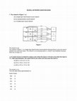The test data was produced in the same way as described above, but only leaving the first letter of every 19 621 AssociativeSelf-Organizing Self-Organizing Map Associative Map I 100% 100% I U3 A 100% 80% U2 100% 100% 100% U A 100% D 50% 3% 50% 20x20 41% 15x15 50% 99% 90% G B U1 100% D 100% 100% 100% 100% 100% 100% 86% 10x10 I 100% D G B A 50% B 88% 25x25 I U 50% G 11% D A 100% B U 100% G Fig. 12. Left: An example of an ideal state diagram for three sequences of length 5. Right: State diagrams for networks with 10 × 10, 15 × 15, 20 × 20 and 25 × 25 nodes. sequence untouched and changing the others to null vectors (thus simulating no input at all). For every test iteration the coordinates of the winner neuron on the A-SOM surface were recorded. Then we analysed the sequential order of the winners by generating state diagrams. A state diagram can visualize a systems behaviour by specifying a number of states that the system may be in, as well as possible transitions between these states. A state diagram is generally drawn as a number of boxes, representing states, and arrows, representing the transitions. We label transitions with a percentage, indicating the probability for that transition compared to all transitions from the same source state. This means that our state diagrams are graphical representations of non-deterministic finite state machines, or what is also referred to as Markov chains. An example of an ideal state diagram for three sequences of length 5 is shown to the left in Fig. 12. There will of course also be transitions from the topmost states to the bottom states (from the last letter of each sequence to the first letter of each following sequence), with, on average, a transition probability of 33%. However, these have been left out since they only indicate the start of a new sequence. 4.2.1 Different lengths, same vowels The first experiment was a replication of one of Elman (1990) experiment where the network was trained on sequences representing ’ba’, ’dii’ and ’guuu’. That is, three sequences starting with a unique consonant followed by one, two or three of the same vowel. For these experiments, validation was made to find out which winner neuron corresponded to which letter in the sequences. This was done by simply giving the letters as input and registering which neuron was the winner for each letter. The A-SOM was then tested with test data constructed in the same way as the training data but with the vowels substituted with null vectors, as described above. The state diagrams for this experiment is shown to the right in Fig. 12 for four different sizes of the A-SOM; 10 × 10, 15 × 15, 20 × 20 and 25 × 25. To make the diagrams more readable, only the correct connections have been included. As an example of the activity in this experiment, Fig. 13 (left) shows the activity of the network one iteration 20 622 Self- Organising NewAlgorithm Achievements Self Organizing Maps ApplicationsMaps, and Novel Design Fig. 13. Left: Activity pattern one iteration after presenting a ’B’ in the first experiment with same vowels, different lengths. Right: Activity patterns for sequences in the experiment with same length and same vowels. after presenting it with the letter B. The validated areas are shown with arrows. The letter ’u’ is represented in two places (they both are activated when validating), as is ’i’, but ’i’ elicit maximum activity in different areas based on its position in the sequence, as indicated by i1 and i2 . In Fig. 13 (left) we can also see that there is a black spot in the lower left corner where there is no activity at all. One interpretation of this is that the network has learnt that a ’B’ never follows an ’a’. One can also see that there is a little bit of activity in the rest of the network, even in parts that do not seem to represent any letter at all. The reason for this could be that for the lower left ’B’ to be entirely void of activity, there need to be activity elsewhere to make that part have relatively lower activity, i.e. activity must be relative to all other activity. 4.2.2 Same length, same vowels Having run Elman’s original test, the experiment was modified so that the sequences were of equal length. They were all set to be three letters long; one consonant and two equal letters (’baa’, ’dii’ and ’guu’). The analysis of this experiment was different. Pictures were taken of the total activity of the network and assembled into a composite image so that the sequences of activity could be visualized easily. This was done to make a qualitative analysis of interesting ways in which the network represent different relations between states. Fig. 13 (right) shows the activity of the network in the test of this experiment. In Fig 13a, the activity patterns of the network are grouped by sequence, to enable comparisons within sequences, whereas Fig 13b enables comparisons between sequences. One can see that activity patterns are distinct from each other for different positions even though the letter is the same (horizontally compare the first ’a’ and second ’a’ following a ’B’ in Fig 13a.), though very similar for the same position between different trials (vertically compare the first ’a’s in Fig 13a). 4.2.3 Same length, unique vowels In the third experiment all sequences had the same length and all vowels were different, even within sequences. Note that we use the word vowel here to mean an element in the sequence, there is no connection to alphabetical vowels. The length of the sequences ranged from 2 to 19 elements. The aim here was to find the smallest network that could represent sequences of 21 623 AssociativeSelf-Organizing Self-Organizing Map Associative Map 2500 y=18,268e0,214x R2=0,975 2000 1500 1000 500 9 12 15 18 21 24 27 30 33 36 39 42 45 48 51 54 57 Fig. 14. Graph plotted for the number of nodes in smallest network with regard to the total number of letters in the sequences. each length with 100% correctness or very close to it. To speed up this process we made the assumption that the minimum network size would not decrease when increasing the sequence length. That is, for a new sequence length the initial network size tested was the network size of the previously run test. It has turned out that this assumption does not hold strictly. In one training trial it was discovered that a network of 9 × 9 nodes was able to represent the sequences, while a network of 10 × 10 nodes performed worse. So even though the required network size seemed to increase with increased sequence length overall, there are minor local variations to this rule. This may simply be the effect of random variations in training data or the initial connection weights. No validation was made for whether the sequence of winners from the testing was in the correct order. Only the pattern of states and their transitions percentages were used and it was manually tested whether the state diagram fitted with an ideal diagram, as shown in Fig. 12 (left). This should not be a problem since it would be extremely unlikely that an incorrect state transition would have a probability of 100%. When running the trial where the sequence length was nine, no network seemed to be able to represent the sequences fully. Sizes up to 25 × 25 nodes were tried without success. It is worth mentioning that sequences of length eight only required 9 × 9 nodes. But, regenerating the test and training data and running the trial again relieved the matter and a 9 × 9 network was found that performed 100%. This could indicate that the network is sensitive to the training and test data, but to be certain further research should be done on the difference between these two training/test-sets. Running the experiment with every trial having three sequences of the same length and all unique letters, and then plotting the smallest network size that could represent the sequences, produced the graph seen in Fig. 14. The graph shows that the number of nodes in the smallest network is exponential with regard to the number of total letters of the sequences in the trial. 4.2.4 Discussion A simplification that has been made in these experiments to make analysis faster as well as more straightforward, has been to use only the sequence of winner neurons. Other activity of the network has thus been ignored. As one can see in Fig. 13 (left), the top area of the network (the ’a’) is the winner here, but there is still much activity in other parts of the network. This can also be seen in the activity sequence series, Fig. 13 (right), where the same letter in different positions of the sequence exhibit different activity patterns. These same letter patterns have 22 624 Self- Organising NewAlgorithm Achievements Self Organizing Maps ApplicationsMaps, and Novel Design distinct winners. This means that it is not completely satisfying to only record the winner neurons. What one would want, rather, is to use the entire activity pattern instead of only the winner neuron. This would require some method to classify similar activity patterns, while separating not too similar patterns. Incidentally, this is a very suitable task for a regular SOM and we could thus use the activity of the A-SOM as input to a separate SOM, an analysis SOM, that would classify the activity of the A-SOM. Then the winner neurons of the analysis SOM, rather than the A-SOM, could be used to determine whether the sequences had been learnt. 5. Conclusion We have presented a novel variant of the Self-Organizing Map called the Associative Self-Organizing Map (A-SOM), which develops a representation of its input space but also learns to associate its activity with the activities of an arbitrary number of (possibly time delayed) ancillary inputs. The A-SOM has been explored in several experiments. In one experiment we connected an A-SOM to two ancillary SOMs and tested with randomly generated points from a subset of the plane. The system in this experiment could be seen as a model of a neural system with two monomodal representations (the two SOMs) and one multimodal representation (the A-SOM) constituting a neural area that merges three sensory modalities into one representation. In another experiment we used the A-SOM in a bimodal self-organizing system for object recognition which used real sensors for the haptic submodalities hardness and texture. The results from this experiment are encouraging. The system turned out to be able to discriminate individual objects based on input from each submodality as well as to discriminate hard from soft objects. More importantly, the input to one submodality has shown to be sufficient to trigger an activation pattern in the other submodality, which resembles the pattern of activity the object would yield if explored with the sensor for this other submodality. In other experiments we explored the ability of the A-SOM to learn sequences and we presented an A-SOM based bimodal model of internal simulation, and tested its ability to continue with reasonable sequences of activity patterns in its two A-SOMs in the absence of any input. It is worth noting that although so far it has not been tested the authors can see no impediments to why it should not be possible to have several sets of connections that feed back the total activity of the A-SOM to itself as ancillary input but with varying lengths of the time delays. This would probably yield an enhanced ability for internal simulation and to remember perceptual sequences (at the cost of more computations). Among other unsupervised recurrent architectures the Recursive SOM (Voegtlin, 2002) is probably the most similar to an A-SOM with recurrent connections. It is worth commenting on some similarities and differences. The two architectures mainly differ in the way a winner neuron is selected. The selection of a winner in the Recursive SOM depends on both the input vector and the time delayed feedback activity. This is not the case for the A-SOM, where the winner selection depends only on the input vector. Because of this, a reasonable guess would be that the A-SOM with recurrent connections would perform better than the Recursive SOM in classification of single inputs when not considering where in the sequence it comes. This is so because the organization of the A-SOM is completely independent of the recurrent input. The recurrent connections in the A-SOM are ancillary connections, which means there is a separate set of weights that during learning are adjusted to produce ancillary activity that is similar to the main activity. There might of course also be some disadvantages with the AssociativeSelf-Organizing Self-Organizing Map Associative Map 23 625 A-SOM with recurrent connections when compared to the Recursive SOM. This would need further investigation. The A-SOM actually develops several representations, namely one representation for its main input (the main activity) and one representation for each of the ancillary neural networks it is connected to (the ancillary activities), and one representation which merges these individual representations (the total activity). One could speculate whether something similar could be found in cortex, perhaps these different representations could correspond to different cortical layers. 6. Acknowledgements This work was supported by the Swedish Linnaeus project Cognition, Communication and Learning (CCL), funded by the Swedish Research Council. 7. References Balkenius, C., Moren, J., Johansson, B. & Johnsson, M. (2010). Ikaros: Building cognitive models for robots, Advanced Engineering Informatics 24(1): 40–48. Bartolomeo, P. (2002). The relationship between visual perception and visual mental imagery: a reappraisal of the neuropsychological evidence, Cortex 38: 357–378. Bishop, C. M. (1995). Neural Networks for Pattern Recognition, Oxford University Press. Carpenter, G., Grossberg, S., Markuzon, N., Reynolds, J. & Rosen, D. (1992). Fuzzy ARTMAP: A neural network architecture for incremental supervised learning of analog multidimensional maps, IEEE Transactions on Neural Networks 3: 698–713. Chappell, G. J. & Taylor, J. G. (1993). The temporal kohonen map, Neural Networks 6: 441–445. Consortium, I. H. G. S. (2004). Finishing the euchromatic sequence of the human genome, Nature 431(7011): 931–945. Elman, J. (1990). Finding structure in time, Cognitive Science 14(2): 179–211. Hesslow, G. (2002). Conscious thought as simulation of behaviour and perception, Trends Cogn Sci 6: 242–247. Johnsson, M. & Balkenius, C. (2008). Associating SOM representations of haptic submodalities, in S. Ramamoorthy & G. M. Hayes (eds), Towards Autonomous Robotic Systems 2008, pp. 124–129. Johnsson, M., Balkenius, C. & Hesslow, G. (2009a). Associative self-organizing map, International Joint Conference on Computational Intelligence (IJCCI) 2009, pp. 363–370. Johnsson, M., Balkenius, C. & Hesslow, G. (2009b). Neural network architecture for crossmodal activation and perceptual sequences, Papers from the AAAI Fall Symposium (Biologically Inspired Cognitive Architectures) 2009, pp. 85–86. Kohonen, T. (1988). Self-Organization and Associative Memory, Springer Verlag. Kohonen, T. (1990). The self-organizing map, Proceedings of the IEEE, 78, 9, pp. 1464–1480. Kosslyn, S., Ganis, G. & Thompson, W. L. (2001). Neural foundations of imagery, Nature Rev Neurosci 2: 635–642. McGurk, H. & MacDonald, J. (1976). Hearing lips and seeing voices, Nature 264: 746–748. Miikkulainen, R., Bednar, J. A., Choe, Y. & Sirosh, J. (2005). Computational maps in the visual cortex, Springer. Mountcastle, V. (1997). The columnar organization of the neocortex, Brain 120(4): 701–722. Nguyen, L. D., Woon, K. Y. & Tan, A. H. (2008). A self-organizing neural model for multimedia information fusion, International Conference on Information Fusion 2008, pp. 1738–1744. 24 626 Self- Organising NewAlgorithm Achievements Self Organizing Maps ApplicationsMaps, and Novel Design Strickert, M. & Hammer, B. (2005). Merge som for temporal data, Neurocomputing 64: 39–71. Tan, A. H. (1995). Adaptive resonance associative map, Neural Networks 8: 437–446. Varsta, M., Millan, J. & Heikkonen, J. (1997). A recurrent self-organizing map for temporal sequence processing, ICANN 1997. Voegtlin, T. (2002). Recursive self-organizing maps, Neural Networks 15: 979–991.