www.nature.com/scientificreports
OPEN
Received: 7 June 2018
Accepted: 27 March 2019
Published: xx xx xxxx
Environmental predictors of
habitat suitability and occurrence
of cetaceans in the western North
Atlantic Ocean
Samuel Chavez-Rosales1, Debra L. Palka2, Lance P. Garrison3 & Elizabeth A. Josephson1
The objective of this study was to identify the main environmental covariates related to the abundance
of 17 cetacean species/groups in the western North Atlantic Ocean based on generalized additive
models, to establish a current habitat suitability baseline, and to estimate abundance that incorporates
habitat characteristics. Habitat models were developed from dedicated sighting survey data collected
by NOAA- Northeast and Southeast Fisheries Science Centers during July 2010 to August 2013. A group
of 7 static physiographic characteristics and 9 dynamic environmental covariates were included in the
models. For the small cetacean models, the explained deviance ranged from 16% to 69%. For the large
whale models, the explained deviance ranged from 32% to 52.5%. Latitude, sea surface temperature,
bottom temperature, primary productivity and distance to the coast were the most common covariates
included and their individual contribution to the deviance explained ranged from 5.9% to 18.5%. The
habitat-density models were used to produce seasonal average abundance estimates and habitat
suitability maps that provided a good correspondence with observed sighting locations and historical
sightings for each species in the study area. Thus, these models, maps and abundance estimates
established a current habitat characterization of cetacean species in these waters and have the
potential to be used to support management decisions and conservation measures in a marine spatial
planning context.
The Northeastern coast of the United States is one of the most populated portions of the country and supports
some of the highest intensity of shipping, fishing and marine development in the nation. Not only has ocean
use increased dramatically during the past 40 years, but the underlying marine ecosystem has also experienced
changes in ocean water temperatures1.
A number of cetacean species listed in the Endangered Species Act (ESA) and protected by the Marine
Mammal Protection Act (MMPA) are subject to these environmental and anthropogenic pressures2. Cetaceans
play important roles in the marine ecosystems as predators whose dynamics are associated with the mid-trophic
levels through trophic linkage3. Consequently, these species not only affect entire food webs, but are also affected
by the dynamics of the physical and biological environment4,5. Detailed current knowledge of the distributions
of cetaceans and their suitable habitat is important for the effective management and conservation not only of
cetacean species but also of entire marine ecosystems3. This is particularly important given the rapidly changing
oceanic environment in the Northwest Atlantic Ocean off the U.S.6 and the increasing demands for energy production that promoted the development of renewable energy areas on the outer continental shelf7.
Results from habitat suitability models, their underlying spatial-temporal density distribution maps and the
relationships between habitat features and density patterns are a cornerstone to support conservation and management. For example, they can be used to predict and monitor species’ response to changes in the climate and
anthropogenic impacts8,9, and generate abundance estimates that support conservation and management10,11. In
addition, these models have the potential to identify priority conservation areas, and diversity hot or cold-spots12.
Several U.S. federal agencies require information about spatial-temporal density, habitat, abundance, population
1
Integrated Statistics, 16 Sumner Street, Woods Hole, MA, 02543, USA. 2NOAA Northeast Fisheries Science Center,
166 Water Street, Woods Hole, MA, 02543, USA. 3NOAA Southeast Fisheries Science Center, 75 Virginia Beach Drive,
Miami, FL, 33149, USA. Correspondence and requests for materials should be addressed to S.C.-R. (email: schavez@
integratedstatistics.com)
SCIENTIFIC REPORTS |
(2019) 9:5833 | https://doi.org/10.1038/s41598-019-42288-6
1
www.nature.com/scientificreports/
www.nature.com/scientificreports
Figure 1. Effort track lines in the AMAPPS study area during 2010–2013, most track lines were surveyed
multiple times by shipboard and aerial surveys. Renewable energy areas include a 10 km buffer zone.
size and predictive models for marine protected species to support their environmental compliance documentation related to the National Environmental Policy Act (NEPA), MMPA and ESA. For example, the U.S.
Department of Energy and the U.S. Bureau of Ocean Energy Management are working closely with several states,
to establish offshore renewable energy developments within 50 miles of the eastern U.S. coastline on the outer
continental shelf7. Other examples are regulations under the MMPA to govern the unintentional taking of marine
mammal incidental to training and testing activities conducted by the U.S. Navy13. In both of these examples,
identifying suitable habitat would help constituents to determine how to minimize human and cetacean interactions and an important component of their respective Environmental Impact Statements.
The objective of this study was to provide this background information for the above conservation and management needs; specifically, to use generalized additive models to establish a current habitat suitability description for cetacean species, to identify the main environmental covariates related to cetacean distribution, and to
estimate abundance accounting for habitat relationships. Further, and example application of these models in
conservation and management issues is discussed.
Results
Habitat models.
A total of 103,395 km of track line was divided into 13,792 spatial-temporal cells (3,329 for
spring, 5,978 for summer, 3,237 for fall and 1,248 for winter) that covered offshore and coastal habitats including the renewable energy areas (Fig. 1, Supplementary Table S1 previously reported in Palka et al.)14. A total of
3,158 sightings of cetacean species/groups were available for 1,413 of these spatial-temporal cells (273 for spring,
796 for summer, 257 for fall and 87 for winter). The species/groups sightings per season are summarized in
Supplementary Table S2, (previously reported in Palka et al.)14 and the environmental covariates are summarized
in Supplementary Table S3. Information related to effort and seasonal sightings were previously reported in Palka
et al.14.
A total of 19 season/species predictive models were developed, which included 10 single species models using
data from all seasons combined (spring, summer and fall), 6 species/group models using data from summer
only, and 3 models for harbour porpoise which had sufficient sample size to develop separate seasonal models
to explain fine scale seasonal migration for spring, summer and fall. Due to low effort and low animal density
detected for most of the species, the winter data was not included in the model development, with the exception
of the model for common bottlenose dolphin where sufficient numbers of animals were detected.
The most parsimonious model for each species included 4–6 different environmental covariates. The total
deviance explained by the models ranged from 16.2% for the summer model of Atlantic spotted dolphin to 69.3%
for the summer model of harbour porpoise. Overall, latitude and SST were included in 67% and 61% of the models respectively, followed by bottom temperature, primary productivity and sea floor slope in 39% of the models.
SCIENTIFIC REPORTS |
(2019) 9:5833 | https://doi.org/10.1038/s41598-019-42288-6
2
www.nature.com/scientificreports
www.nature.com/scientificreports/
Generalized Additive Model Terms
SPECIES
SST
BT
Beaked whale, Cuvier’s (summer)
1.13
11.08
Beaked whale, Sowerby’s (summer)
6.49
Beaked whale group (summer)
0.80
Common bottlenose dolphin
(spring, summer, fall and winter)
0.4
Atlantic spotted dolphin (summer)
PP
3.59
Fin whale
Total DE
CHL PIC POC SAL MLD SLA
2.52
3.43
7.86
Harbour porpoise (spring)
0.98
Humpback whale
9.14
4.70
6.48
0.65
0.19
5.88
Risso’s dolphin
6.12
Sei whale
20.18
Common dolphin
14.53
Sperm whale
7.24
10.07 5.35
Striped dolphin (summer)
6.79
41.52 1.39
White-sided dolphin
4.38
13.22
10.21
5.67
34.7
4.39
2.03
42.97
10.21
49.9
66.6
5.66
0.80
31.9
2.65
5.65
3.57
6.39
56.2
20.25 11.16
49.6
24.76 3.87
9.39
10.53
52.5
7.64
9.49
2.90
1.02
42.1
33.5
3.12
2.63
33.7
39.9
21.73
3.69
1.35
22.3
69.3
10.70
6.53
2.88
10.06
28.27
4.51
11.97
41.1
60.17 2.95
0.57
9.59
5.76
7.02
38.1
1.48
9.97
1.41
Short/Long-finned pilot whale group
0.56
22.96
10.80
Dwarf/Pygmy sperm whale group
(summer)
Minke whale
13.64 23.11
34.0
15.79
1.48
2.62
6.79
40.87
Harbour porpoise (summer)
D125 D200 D1000 te(LAT, BT) %
16.2
10.92 4.08
1.02
2.60
Harbour porpoise (fall)
DEPTH SLOPE D2S
6.66
1.09 3.54
3.11
LAT
7.57
52.8
18.5
Table 1. Percent deviance explained (DE) by term for each species model. The data input for the models cover
spring, summer and fall seasons unless is specified in parenthesis. All the model terms were significant at
p < 0.05 by a Wald-type test of f = 054.
The least frequent predictors included in the models were particulate organic carbon and sea surface height
anomaly both with 5.6%. (Table 1).
Habitat suitability maps generated from the model outputs identified clear differences in the core habitat for
the species that have the tendency to converge in the same space and time, giving indications of habitat partition
(Supplementary Figs S1 to S17).
Goodness-of-fit measures of the models were determined to be adequate as evaluated in two ways. First, overall the models fitted the input data well according to the Spearman’s rank correlation, mean absolute error, and
mean absolute percent error statistics, using both the non-zero input data and cross-validation methods (Table 2).
Second, a comparison of habitat suitability maps to field sighting locations revealed a good correspondence
between the model predictions and observed data used to develop the models (Supplementary Figs S1 to S17).
Distribution-abundance connection with environmental covariates. Partial regression smooth
plots generated by the habitat models provided a good metric of the physical and biological habitat of these
species, and represent how animal abundance changes relative to its mean in response to changes in each
model covariate term. For example, the relationship between dolphin abundance and sea surface temperature
showed well-defined thermal habitats that provide evidence of habitat partitioning (Fig. 2). This is illustrated
by white-sided and bottlenose dolphins who are found more frequently in cooler waters, peaking at about 10 °C
and 12 °C, respectively. Common and striped dolphins are found in warmer waters peaking at about 16 °C and
20 °C, respectively. In contrast, Risso’s dolphins are found most often in the warmest waters that are over 20 °C.
The partial regression plots of sea surface temperature also provided information on the range of temperatures
commonly used by the species. For example, common dolphins are found in waters with a wider range of temperatures (5–24 °C) in contrast to striped dolphins (14–25 °C).
The habitat covariates in the models were able to capture seasonal movement patterns and fine scale distribution patterns by including not only static covariates, like latitude, but also dynamic environmental covariates
that change over the seasons and on a finer scale. For example, both humpback and minke whales have similar
patterns in the partial regression relationships for sea surface temperature (Fig. 2) and latitude (Fig. 3). However,
the humpback model also includes chlorophyll a and the minke whale model includes particulate organic carbon
which aggregates phytoplankton, zooplankton, bacteria and detritus, suggesting a difference in trophic relationships and also resulting in very different habitat suitability patterns (Table 1, Supplementary Figs S8 and S10).
Abundance estimates.
Average seasonal abundance estimates derived from the habitat suitability models for the entire study area for all the cetacean species and species guilds are found in Table 3, these estimates
were previously reported in Palka et al.14. For species that were detected during spring, summer and fall, various
distribution and abundance patterns were observed. For the pilot whale, beaked whale, and Kogia groups, the
abundance estimates were developed for the guild and not for individual species. In addition sightings of Kogia
SCIENTIFIC REPORTS |
(2019) 9:5833 | https://doi.org/10.1038/s41598-019-42288-6
3
www.nature.com/scientificreports
www.nature.com/scientificreports/
Non-Zero Input Data
Species
RHO
MAE
Atlantic spotted dolphin
0.273
0.199
Cuvier’s beaked whale
0.091
0.013
k cross-validation k = 25
MAPE
RHO
MAE
87.861
0.113
0.195
MAPE
86.271
86.030
0.219
0.017
85.129
Sowerby’s beaked whale
0.379
0.003
92.233
0.151
0.004
93.303
Unidentified beaked whales
0.429
0.013
81.191
0.173
0.013
85.211
Common bottlenose dolphin
0.315
0.411
77.602
0.203
0.421
82.069
Fin whale
0.117
0.009
88.725
0.129
0.009
89.992
Harbour porpoise - Fall
0.179
0.038
85.778
0.189
0.047
78.802
Harbour porpoise - Spring
0.242
0.049
87.975
0.175
0.049
87.068
Harbour porpoise - Summer
0.260
0.113
80.405
0.209
0.102
79.875
Humpback whale
0.278
0.003
91.975
0.085
0.004
91.612
Pygmy/dwarf sperm whale
0.404
0.017
82.288
0.203
0.016
82.218
Minke whale
0.500
0.006
94.595
0.087
0.005
95.775
Long/short pilot whale
0.530
0.074
88.925
0.146
0.065
95.085
Risso’s dolphin
0.103
0.054
85.387
0.187
0.052
99.327
Sei whale
0.239
0.004
87.176
0.078
0.004
89.865
Common dolphin
0.192
0.277
104.383
0.183
0.324
105.963
Sperm whale
0.227
0.006
82.018
0.145
0.005
81.383
Striped dolphin
0.290
0.065
76.438
0.235
0.074
128.025
White-sided dolphin
0.314
0.303
86.471
0.064
0.265
92.461
Table 2. Results of diagnostic tests to evaluate fit of the habitat models. RHO = Spearman’s rank correlation
coefficient; MAE = Mean absolute error; MAPE = Mean absolute percentage error. Fit threshold values were
taken from Kinlan et al.49 where:
RHO: Poor = x < 0.05 Fair to good = 0.05 < = x < 0.3
Excellent = x > 0.3
MAE: Poor = x > 1
Fair to good = 1 > = x > 0.25
Excellent = x < = 0.25
MAPE: Poor = x > 150% Fair to good = 150% > = x > 50% Excellent = x < = 50%.
Figure 2. Examples of the partial effect of SST (°C) on the changes in abundance relative to its mean for common
dolphin (CODO), white-sided dolphin (WSDO), common bottlenose dolphin (BODO), Risso’s dolphin
(GRAM), striped dolphin (STDO), humpback whale (HUWH), minke whale (MIWH), sei whale (SEWH).
SCIENTIFIC REPORTS |
(2019) 9:5833 | https://doi.org/10.1038/s41598-019-42288-6
4
www.nature.com/scientificreports/
www.nature.com/scientificreports
Figure 3. Examples of the partial effect of latitude on the changes in abundance relative to its mean for
common dolphin (CODO), Atlantic spotted dolphin (ASDO), humpback whale (HUWH), minke whale
(MIWH), fin whale (SEWH), Sowerby’s beaked whale (SBWH) and Cuvier’s beaked whale (CBWH).
spp., beaked whales and striped dolphins occurred in habitats further offshore in regions only the shipboard surveys were able to access during summer. Consequently, the estimate of abundance for these species/groups only
represents the summer season.
Robustness validation.
The models were also shown to be robust as defined by comparing the predicted model values to the data that were collected at times different than the data used to develop the models.
Specifically, a total of 386 sightings were not included in the development of the models for humpback whale, fin
whale, sperm whale, short/long-finned pilot whale, Risso’s dolphin, common dolphin and common bottlenose
dolphin collected during spring 2014, were located within the core habitat regions as predicted by the habitat
models when applied to the values of the covariates for the spring of 2014 (Supplementary Figs S18 to S24). In
further analysis only for common dolphin, the 2010-2013 model definition applied to the 2004 summer environmental covariates predicted an abundance estimate that was less than 1% greater (not statistically different) than
the previously reported 2004 abundance estimate when corrected for availability bias (Table 4). The previously
reported 2004 estimate15 was produced from only data collected by shipboard and aerial surveys during summer
of 2004. Even though the species distribution patterns detected during the surveys between summer 2004 and
spring 2014 were quite different, the predicted habitat suitability maps matched the common dolphin sightings
distribution recorded for both seasons and years (Fig. 4). Further indications of model fit are found in Palka
et al.14 where the results from the goodness-of-fit tests of each the modelling steps are provided. In addition
visual comparisons of the predicted seasonal density maps and locations of historical sightings since 1970 from
OBIS-SEAMAP16 are also provided.
Discussion
Federal agencies like U.S. Department of Energy, National Marine Fisheries Service, U.S. Fish and Wildlife
Service, BOEM, and U.S. NAVY and other ocean developers require information from a diverse suite of topics such as density/abundance, distribution, stock structure, life history, behaviour, habitat use, environmental
drivers, impact assessment and spatial modelling to support their mandates. Habitat models and model outputs
presented in this paper provide some of the background information need by those agencies for spatial planning
and conservation purposes and are available in a user friendly interface as a part of the AMAPPS model viewer
at www.nefsc.noaa.gov/AMAPPSviewer. First, we will discuss the development of the models, and then compare
these models to other developed in the same general region, then finally potential uses of the model results.
SCIENTIFIC REPORTS |
(2019) 9:5833 | https://doi.org/10.1038/s41598-019-42288-6
5
www.nature.com/scientificreports
www.nature.com/scientificreports/
Species
Spring (Mar- May)
Summer (Jun-Aug)
Fall (Sep-Nov)
Atlantic spotted dolphin
65,948 (0.16)
54,731 (0.15)
56,372 (0.16)
Beaked whale, Cuvier’s
3,425 (0.3)
Beaked whale, Sowerby’s
676 (0.38)
Beaked whale group
6,523 (0.17)
Common bottlenose dolphin*
111,729 (0.38)
138,728 (0.37)
104,993 (0.24)
Fin whale
3,817 (0.15)
4,718 (0.13)
4,514 (0.12)
Harbour porpoise (spring)
30,126 (0.2)
Harbour porpoise (summer)
83,250 (0.18)
Harbour porpoise (fall)
17,943 (0.49)
Humpback whale
1,510 (0.23)
1,246 (0.17)
Dwarf/Pygmy sperm whale group
1,399 (0.17)
10,632 (0.18)
Minke whale
1,484 (0.57)
2,834 (0.25)
2,829 (0.25)
Short/Long-finned pilot whale group
26,441 (0.4)
24,670 (0.3)
29,559 (0.3)
Risso’s dolphin
12,759 (0.21)
36,785 (0.2)
29,093 (0.21)
Sei whale
4,500 (0.42)
1,244 (0.47)
1,176 (0.48)
Common dolphin
111,042 (0.22)
118,697 (0.21)
183,510 (0.19)
Sperm whale
4,766 (0.33)
3,667 (0.14)
3,557 (0.15)
Striped dolphin
81,512 (0.12)
White-sided dolphin
47,371 (0.49)
42,985 (0.46)
44,277 (0.39)
Table 3. Average seasonal abundance estimates derived from the 2010–2013 habitat models with its associated
coefficient of variation in parenthesis. These estimates were previously reported in Palka et al.14.
Source
Survey
CNbest
CV
Garrison et al.55
Shipboard Jun-Aug 30,196 1.00
Season
Nbest
ABC*
30,196
0.54
Palka et al.56
Shipboard Jun-Aug 35,263 1.00
35,263
0.50
Palka et al.56
Aerial
59,445
0.24
SAR 200515 (sum of the above)
124,904
0.23
Habitat model**
126,009
0.10
Jun-Aug 55,284 0.93
Table 4. Robustness validation results of the common dolphin model. Common dolphin abundance estimates
for 2004 by platform and the abundance estimate derived from the habitat model which includes the availability
bias correction. Nbest = Abundance estimate; ABC = Availability bias correction factor; CNbest = Abundance
estimate corrected for availability bias; CV = Coefficient of variation. *Palka et al.14. **2010–2013 model
definition, with June to August 2004 sea surface temperature data.
Partial regression smooth plots of the animal density in relation to SST and latitude generated by the models
are in agreement with the current knowledge of the species distributions17,18. Despite model uncertainty, the
robustness validation supported the predictive inferences of the models tested and expanded the potential application to detect species shifts in response to habitat changes. Though the amount of deviance explained is comparable to similar studies, improved deviance explained may be possible if additional physical and biological
environmental covariates were included, such as fronts due to temperature, salinity and primary productivity, and
densities of forage fish or other potential prey species.
One important assumption about regression type models, like those presented in this document, is that the
models assume the link between animal density and habitat factors have consistent statistical relationships within
the spatial-temporal variables included in the model. Given this assumption, it is then possible to predict the average density in locations or time periods where surveys did not actually occur19. However, if those proxies are unable to detect changes in the underlying ecological processes through time and space, then those assumptions are
no longer valid. This means that a causal or mechanistic relationship is not explicitly assumed. Consequentially,
the type of model used in this document provides an average pattern of the habitat suitability and abundance.
Comparison with previous studies in the region.
This effort is not the first of its kind for the western
North Atlantic waters. The evolution of the theoretical and computational improvements related to modelling
animal density is evident by the past and present efforts that have used line transect sightings data collected by the
NEFSC and SEFSC. Hamazaki17 used multiple logistic regression to model the presence/absence of sightings from
1990–1996 with oceanographic and topographic variables to predict habitat maps. The U.S. Department of the
Navy20,21 used sightings data from 1998–2005 in generalized additive density surface models to predict the density
in a prediction grid, where g(0) was assumed to be one. The habitat suitability maps and abundance estimates
presented in this document were generated with additional data that were not used in previous studies, and built
upon past efforts. Most recently Roberts et al.11 used data from 1992–2014 to develop habitat-based climatological
SCIENTIFIC REPORTS |
(2019) 9:5833 | https://doi.org/10.1038/s41598-019-42288-6
6
www.nature.com/scientificreports/
www.nature.com/scientificreports
Figure 4. Robustness validation results of the common dolphin habitat model. Habitat suitability for (A)
summer 2004; and (B) spring 2014 overlapped with the actual species sightings for the correspondent season
and year. These sightings were not included in the habitat model development.
density maps and abundance estimates, where g(0) was not assumed to be one; though none of the data used in
the current paper were used in the Roberts et al.11 models. In all of these efforts, the modelling approaches used
the best available data and make logical assumptions and decisions.
Though making a direct comparison between these studies is a complex task, it is important to establish some
of the fundamental differences between Roberts et al.11 and the present paper which include: (A) Differences in
spatial and temporal coverage: most of the data used to develop the Roberts et al.11 models used data that were
collected mostly from 1995 to 2009 (though there are some data from some species up to 2014) and did not
include the data used in this paper, in addition the data were from surveys ranging from the US Pacific to Europe
collected by multiple organizations and methods. In contrast, the models developed in this paper only use data
from the area of interest. (B) Differences in analysis strategies and methods: to standardize all surveys used in
Roberts et al.11 it was necessary to restrict data collected by only one sighting team per platform. Consequently,
to correct for perception and availability bias, when local information was not available, it was necessary to apply
correction factors from surveys conducted in the Pacific Ocean, Eastern Atlantic and Gulf of Mexico, which may
result in unrepresentative corrections because of differences between the survey methods and animal’s behaviour.
Finally, the current analyses also accounted for availability bias by estimating species-specific correction factors,
some of which were estimated from recently tagged animals within the study area14. Another difference was the
way the covariates were processed. For example, Robert’s developed climatological covariates which were a mean
from 1995 to 2014 for a specific time period, say 8-days. In contrast, in the current paper the covariates were an
average over a time period (8-days) from only the same year as the sighting observation. And (C) difference in
presentation: average annual and monthly density-surface maps and abundances were presented in Roberts et
al.11, in contrast to average seasonal estimates and the habitat suitability for the species presented in this study.
In general, the average annual estimates from Roberts et al.11 are the most different from the seasonal estimates
presented in this document for species that migrate out of US waters during some parts of the year, or for species
that changed their seasonal spatial distribution patterns over the last two decades.
In summary, the two observer teams approach used in the present study that includes data from only the area
of interest allowed the estimation of the perception bias correction from the same data that was used to calculate
the density estimates thus resulting in regionally more representative and current abundance estimates and habitat suitability maps.
Example applications of the habitat models.
Society has increasing demands for energy production
triggering the development of renewable energy areas on the outer continental shelf, currently reaching a total
of 16,149 km2 from Massachusetts to Florida. These areas have a significant overlap with MMPA strategic dolphins and ESA whale species’ habitats and the level of interaction was documented and quantified by the models
(Supplementary Table S4 and Figs S1 to S17). For example, even though most of the waters in the potential renewable energy areas are shallow and close to the shore, the models for pilot whales, Risso’s dolphins, white sided
dolphins, common dolphins and Atlantic spotted dolphins identified the deeper offshore regions of the potential
renewable energy areas as part of their preferred habitat. Interestingly, the model for sperm whales, which are
generally considered deep water animals, predicted very low abundance at the farthest offshore regions of the
SCIENTIFIC REPORTS |
(2019) 9:5833 | https://doi.org/10.1038/s41598-019-42288-6
7
www.nature.com/scientificreports/
www.nature.com/scientificreports
potential renewable energy areas that were either close to the shelf break or extended into deeper waters like those
in Massachusetts/Rhode Island and North Carolina and this has been confirmed by recorded sightings14.
There was a spatial difference in diversity patterns associated with latitude, in which the northern areas were
more diverse in comparison to the southern areas. For example, the Massachusetts/Rhode Island area is located
in a region with the highest species richness and showed the highest estimated abundance of ESA whale species
(humpback, fin, sei and sperm whales) for all seasons. In addition the diversity index changed seasonally driven
by animal migration (Supplementary Table S4). In the rest of the renewable areas the habitats become suitable
for these species only during spring when the whales migrate through. In the case of MMPA strategic dolphins
(harbour porpoises, white-sided dolphins, common dolphins, long/short finned pilot whales and common bottlenose dolphin), Massachusetts/Rhode Island, New Jersey and North Carolina/South Carolina showed the highest
abundance estimates with similar spatial diversity patterns.
Changes in key physical and biological oceanographic features can alter marine ecosystems and atmospheric
patterns. For example, in the Gulf of Maine spatial shifts of species assemblages associated with shallower, warmer
waters tended to shift towards waters with cooler temperatures, while species assemblages associated with relatively cooler and deeper waters shifted deeper, but with little latitudinal change. Species assemblages associated
with warmer and shallower water on the broad, shallow continental shelf from the Mid-Atlantic Bight to Georges
Bank shifted strongly northeast along latitudinal gradients with little change in depth22. Habitat-based cetacean
models such as those developed here will be able to be used to explore the potential changes in the distribution
and abundance of cetaceans relative to the changes to the physical and biological changes.
It is clear that the effects on the movement and extent of species assemblages will hold important implications
for management, mitigation and adaptation on these waters. The models and maps presented in this document
provide a recent habitat characterization of the species discussed, and based on the assumptions and the predictive nature, have the potential to support management decisions and conservation measures in a marine spatial
planning context.
Methods
Study area. The study area ranged from Halifax, Nova Scotia, Canada to the southern tip of Florida; from the
coastline to slightly beyond the US exclusive economic zone and covers approximately 1,193,320 km2 (Fig. 1). It
was subdivided into 10 × 10 km cells and sampled during 16 Atlantic Marine Assessment Program for Protected
Species (AMAPPS) surveys, using NOAA Twin Otter aircrafts in coastal regions and NOAA ships Henry B.
Bigelow by the Northeast Fisheries Science Center (NEFSC), and Gordon Gunter by the Southeast Fisheries
Science Center (SEFSC) in offshore regions. These surveys covered approximately 103,995 km of line-transect
survey effort during July 2010 to August 2013 (Supplementary Table S1). Habitat suitability models were built for
14 species and 3 species guilds (Table 1).
Habitat predictors. Habitat predictors included a suite of static physiographic data and dynamic environmental covariates and were obtained from ETOPO1 1-min global relief data23, AVISO+24, the Hybrid Coordinate
Ocean Model (HYCOM) 25, and from NOAA’s Environmental Research Division Data Access Program
(ERDDAP)26 website (Supplementary Table 3). The environmental data were downloaded from the source using
a bounding box whose extent covered the study area, and subsequently processed using custom code developed in
R (v. 3.1.1)27 with the R packages “raster” (v 2.5-2)28, “ncdf ” (v 1.6.8)29, “rgdal” (v 1.1-6)30, “RNetCDF” (v 1.8-2)31,
“lubridate” (v 1.5.3)32, “RODBC” (v 1.3–10)33 and “geosphere” (v 1.5–1)34. The process included a re-sampling
of the data to the geographical midpoint of each 10 × 10 km stratum using oblique Mercator grid with bilinear
interpolation. When possible, the data were obtained for dynamic covariates on an 8-day basis. Alternatively,
daily images were downloaded and spatially synced to the cells and averaged into 8-day periods. In case of cells
with missing values, a simple interpolation process was applied using the mean from the nearest-neighbour cells,
and if needed the mean from the 8-day period before and after.
Distance Analysis. Samples for modelling animal density were created by dividing the AMAPPS continuous
survey effort into the 10 × 10 km cells. Species-specific information related to the number of sightings and group
size was assigned to each cell. In addition, average sea state and glare within each cell was included as a continuous predictor variable to account for sighting conditions encountered on the surveyed track lines. Line-transect
sightings parameter estimates derived from the surveys were based on effort in Beaufort Sea states from 0 through
435, because the probability of detection decreases as the sea states increases36,37.
The density estimates were based on the independent observer approach assuming point independence38,
calculated using the mark-recapture distance sampling (MRDS) with the computer program Distance (version
6.2)39, for each sampled 10 × 10 km cell using a Horvitz-Thompson-like estimator40. With this approach there was
no need to independently model group size and the error due to extrapolation was minimized. To capture sightability differences between observation platforms and regions, data collected by each aircraft and ship from SEFSC
and NEFSC surveys were analysed independently due to the differences in observers, data collection methods
and habitats surveyed. A traditional MRDS distance analysis was used for the data collected by the shipboard surveys35. Data collected by the aerial surveys were analysed using a two-step process as described by Palka et al.14.
Significant covariates were chosen following the method suggested by Marques & Buckland41 and Laake
& Borchers38. For all of the analyses, the detection probabilities were estimated using right truncated perpendicular distances as suggested in Buckland et al.42 and model selection was based on the goodness-of-fit using
the AIC score (Akaike Information Criterion)43, Chi- squared test, Kolmogorov-Smirnov goodness-of-fit test,
Cramer-von Mises goodness-of-fit test and a visual inspection of the fit, the results of these test are available in
SCIENTIFIC REPORTS |
(2019) 9:5833 | https://doi.org/10.1038/s41598-019-42288-6
8
www.nature.com/scientificreports
www.nature.com/scientificreports/
Palka et al.14. The estimated sighting probability included an estimation of g(0) which is the probability of detecting an animal on the survey track line.
To ensure sufficient sample sizes to accurately estimate model parameters, several similar species were pooled
when needed. The criteria used to define species guilds included shape of the species’ detection functions, general animal behaviour, perceived sightability of the species, and sample size. The estimated global parameters
were applied to the values of the covariates associated with each species in the species group to account for
species-specific detection functions. An overall species-specific abundance estimate was then calculated for each
cells/time period and corrected for species-specific availability bias by platform, as described in Palka et al.14.
The availability bias correction was based on the probability of an animal being detectable at the surface during
a survey, and took into consideration the species diving and aggregation behaviours, in addition to the amount
of time the observer had to analyse any spot of water from each of the survey platforms. This correction tended
to be larger for aerial surveys than for shipboard surveys, and larger for long diving species than for short diving
species.
Modelling. Generalized Additive Models (GAM)44 were developed in R (v. 3.1.1)27 using the package “mgcv”
(v.1.8–6)45. The density estimates for each species/group in sampled cells by the shipboard and aerial surveys were
defined as the response variable. The parameter estimates were optimized using restricted maximum likelihood
criterion and the data were assumed to follow an overdispersed Tweedie distribution46 with null space penalization and thin plate splines with shrinkage47. Further, to avoid overfitting that could render parameter estimates
difficult to interpret biologically, the maximum number of degrees of freedom was limited to 4. Correlations
among environmental covariates ranged from 0.01–0.80 in absolute values. Although “mgcv” is considered to be
robust to such correlations45, variables in a highly correlated pair above r = 0.60, were not used together in the
same model.
Variable selection was performed with automatic term selection48 and a suite of diagnostic tests as proposed
by Kinlan et al.49 and Barlow et al.50. Models with the lowest overall prediction errors and the highest percentage
of deviance explained were selected for further diagnostic testing which included k-fold cross-validation with
25 random data subsets. K-fold cross-validation methods, in contrast to the method where data are partitioned
into separate training and test sets, have the advantage of deriving a more accurate model, especially in cases with
limited sample sizes51, such as in this study.
The relative importance of each term of the final model was estimated by calculating the terms’ approximate deviance explained following the process described by Whitlock et al.52. Briefly, this process involves fitting
a sequence of models to obtain the deviance of the full model, null model and reduced models in which one
smooth term was removed at a time, while retaining the other parameter estimates from the full model constant.
Deviance explained (DE) for each term i was then calculated with the Eq. (1):
D
− DFull model
DEi = i reduced model
Dnull model
(1)
where D is the deviance for a model, and Di reduced model is a model where variable i is omitted.
Following model selection and validation for each of the species, the 2010–2013 average modelled seasonal
(spring, summer and fall) abundance estimates for all cells in the study area were used to generate habitat suitability maps using QGIS (v. 2.10)53.
The habitat suitability (HS) was assumed to be directly correlated with the species’ abundance and distribution. That is, in times and regions with the greatest estimated abundance it was assumed that the habitat was the
most suitable for the species, then using the Eq. (2):
n
HS =
∑ Ni
i
(2)
i was the seasonal estimated abundance for each cell from the species-specific model. The seasonal abunwhere N
dance estimates were calculated by summing the mean predicted abundance of each cell, and the uncertainty
estimates reflect only the uncertainty in the GAM parameter estimates.
Abundance estimates for smaller scale regions within study area that are being considered for development of
offshore renewable energy were also summarized. In some cases it was needed to merge several wind energy lease
areas/wind planning areas together when the areas were relatively small and close together. In addition a buffer
zone was added around all areas in an attempt to designate a generic area in which an animal may be exposed
to due to construction/operation activities within the renewable energy area. The size of an appropriate buffer
is dependent on a variety of factors including species-specific factors, such as natural short-term foraging and
movement patterns which could then influence the animal’s response and sensitivity to the activity. In addition,
the types of activities being undertaken in the offshore renewable energy area, and the physical topography and
oceanographic features have a direct impact on the sound level and propagation. However, for simplicity in this
study, offshore wind energy areas in addition to 10 km buffer zone is referred to as renewable energy areas and is
reflected in the abundance estimates.
Robustness validation of the habitat models was investigated in two ways. First the 2010–2013 model parameters were applied to the spring 2014 environmental data, the resulting predicted habitat suitability was compared
with the actual spring 2014 sightings locations from the AMAPPS surveys. From the species included in this document, only common dolphin, Risso’s dolphin, common bottlenose dolphin, short/long-finned pilot whale, fin
whale, humpback whale and sperm whale were detected during the surveys, thus only the habitat models of these
species were included in the comparison. The second way was by hindcasting the 2010–2013 models by using the
SCIENTIFIC REPORTS |
(2019) 9:5833 | https://doi.org/10.1038/s41598-019-42288-6
9
www.nature.com/scientificreports/
www.nature.com/scientificreports
summer 2004 environmental data. But given the quality of the environmental data needed for the models were
not readily available for the entire study area for 2004, the test was restricted to the common dolphin model. Thus,
the modelled output was compared to not only the summer 2004 sightings locations from a NEFSC abundance
survey but also the abundance estimate reported in the 2005 Stock Assessment Report15 that was derived from
the NEFSC 2004 summer abundance survey data. The work presented in this document conforms to accepted
international ethical standards.
Data Availability
The datasets generated during the current study are available at https://inport.nmfs.noaa.gov/inport/item/23306
under “Distribution information”.
References
1. Ecosystem Assessment Program. Ecosystem Assessment Report for the Northeast U.S. Continental Shelf Large Marine Ecosystem.
US Dept Commer, Northeast Fish Sci Cent Ref Doc. 09–11. Available at, https://www.nefsc.noaa.gov/publications/crd/crd0911/
crd0911.pdf (2009).
2. Perrin, W. F., Würsig, B. & Thewissen, J. G. M. (eds). Encyclopedia of marine mammals. 2nd ed. (Academic Press, 2009).
3. Kanaji, Y., Okazaki, M., Kishiro, T. & Miyashita, T. Estimation of habitat suitability for the southern form of the short-finned pilot
whale (Globicephala macrorhynchus) in the North Pacific. Fish. Oceanogr. 24, 14–25 (2015).
4. Bowen, W. D. Role of marine mammals in aquatic ecosystems. Marine Ecology Progress Series 158, 267–274 (1997).
5. Estes, J. A., Tinker, M. T., Willians, T. M. & Doak, D. F. Killer Whale Predation on Sea Otters Linking Oceanic and Nearshore
Ecosystems. Science 282, 473–476 (1998).
6. Saba, V. S. et al. Enhanced warming of the Northwest Atlantic Ocean under climate change. J. Geophys. Res. Oceans 121, 118–132 (2016).
7. U.S. Department of Energy & U.S. Department of Interior. National Offshore Wind Strategy. DEO/GO-102016-4866 Available at,
https://www.energy.gov/sites/prod/files/2016/09/f33/National-Offshore-Wind-Strategy-report-09082016.pdf (2016).
8. Guisan, A. & Thuiller, W. Predicting species distribution: offering more than simple habitat models. Ecology Letters 8, 993–1009
(2005).
9. Elith, J. & Leathwick, J. R. Species distribution models: ecological explanation and prediction across space and time. Annual Review
of Ecology and Evolutionary Systematics 40, 677–697 (2009).
10. Forney, K., Becker, E., Foley, D., Barlow, J. & Oleson, E. Habitat-based models of cetacean density and distribution in the central
North Pacific. Endang Species Res 27, 1–20 (2015).
11. Roberts, J. J. et al. Habitat-based cetacean density models for the US Atlantic and Gulf of Mexico. Scientific Reports 6, 22615 (2016).
12. Baltensperger, A. P. & Huettmann, F. Predicted Shifts in Small Mammal Distributions and Biodiversity in the Altered Future
Environment of Alaska: An Open Access Data and Machine Learning Perspective. PLoS ONE 10, e0132054, https://doi.org/10.1371/
journal.pone.0132054 (2015).
13. Department of Commerce. Taking and Importing Marine Mammals; Taking Marine Mammals Incidental to the U.S. Navy Training
and Testing Activities in the Atlantic Fleet Training and Testing Study Area. Federal Register Vol. 82, No. 155: 37851 (2017).
14. Palka, D. L. et al. Atlantic Marine Assessment Program for Protected Species: 2010–2014 US Dept. of the Interior, Bureau of Ocean
Energy Management, Atlantic OCS Region, Washington, DC. OCS Study BOEM 2017-071. Available at, https://www.boem.gov/
espis/5/5638.pdf (2017).
15. Waring, G. T., Josephson, E., Fairfield, C. P., & Maze-Foley K. (eds). U.S. Atlantic and Gulf of Mexico Marine Mammal Stock
Assessments – 2005 NOAA Tech Memo 194 Available at, https://www.nefsc.noaa.gov/publications/tm/tm194/ (2006).
16. Halpin, P. N. et al. OBIS-SEAMAP: The Word Data Center for Marine Mammals, Sea Birds, and Sea Turtle Distributions.
Oceanography 22, 104–115 (2009).
17. Hamazaki, T. Spatiotemporal prediction models of cetacean habitats in the mid‐Western North Atlantic Ocean (from Cape Hatteras,
North Carolina, USA to Nova Scotia, Canada). Marine Mammal Science 18, 920–939 (2002).
18. Selzer, L. A. & Payne, P. M. The distribution of white-sided (Lagenorhynchus acutus) and common dolphins (Delphinus delphis) vs.
environmental features of the continental shelf of the Northeastern United States. Marine Mammal Science 4, 141–153 (1988).
19. Guisan, A., Edwards, J. T. C. & Hastie, T. Generalized linear and generalized additive models in studies of species distributions:
setting the scene. Ecological Modelling 157, 89–100 (2002).
20. Department of the Navy. Navy OPAREA Density Estimates (NODE) for the Southeast OPAREAS: VACAPES, CHPT, JAX/CHASN,
and Southeastern Florida & AUTEC-Andros Available at, http://seamap.env.duke.edu/downloads/resources/serdp/Northeast%20
NODE%20Final%20Report.pdf (2007).
21. Department of the Navy. Navy OPAREA Density Estimates (NODE) for the Northeast OPAREAS: Boston, Narragansett Bay and Atlantic
City Available at, http://seamap.env.duke.edu/downloads/resources/serdp/Southeast%20NODE%20Final%20Report.pdf (2007).
22. Kleisner, K. M. et al. The Effects of Sub-Regional Climate Velocity on the Distribution and Spatial Extent of Marine Species
Assemblages. PLoS ONE 11, e0149220, https://doi.org/10.1371/journal.pone.0149220 (2016).
23. Amante, C. & Eakins, B. W. ETOPO1 1 Arc-Minute Global Relief Model: Procedures, Data Sources and Analysis. NOAA Technical
Memorandum NESDIS NGDC-24. National Geophysical Data Center, NOAA. https://doi.org/10.7289/V5C8276M [access date:
11/17/14] (2009).
24. AVISO+. The Ssalto/Duacs altimeter products were produced and distributed by the Copernicus Marine and Environment
Monitoring Service (CMEMS), http://www.marine.copernicus.eu [access date: 11/20/14].
25. Chassignet, E. P. et al. The HYCOM (Hybrid Coordinate Ocean Model) data assimilative system. J. Mar. Syst. 65, 60–83 (2007).
26. Simons, R. A. ERDDAP, http://coastwatch.pfeg.noaa.gov/erddap. Monterey, CA: NOAA/NMFS/SWFSC/ERD [access date:
11/17/14] (2015).
27. R Core Team. R: A language and environment for statistical computing. R Foundation for Statistical Computing, Vienna, Austria,
http://www.R-project.org/ (2014).
28. Hijmans, R. J. & van Etten J. Raster: Geographic analysis and modeling with raster data. R package version 2.0–12, http://CRAN.Rproject.org/package=raster (2012).
29. Pierce, D. ncdf: Interface to Unidata netCDF data files. R package version 1.6.8, http://CRAN.R-project.org/package=ncdf (2014).
30. Bivand, R., Keitt, T. & Rowlingson, B. rgdal: Bindings for the Geospatial Data Abstraction Library. R package version 1.0–4, http://
CRAN.R-project.org/package=rgdal (2015).
31. Michna, P. & Woods, M. RNetCDF: Interface to NetCDF Datasets. R package version 1.8–2, http://CRAN.R-project.org/
package=RNetCDF (2016).
32. Grolemund, G. & Wickham, H. Dates and Times Made Easy with lubridate. Journal of Statistical Software 40, 1–25, http://www.
jstatsoft.org/v40/i03/ (2011).
33. Ripley, B. & Lapsley, M. RODBC: ODBC Database Access. R package version 1.3–10, https://CRAN.R-project.org/package=RODBC
(2015).
34. Hijmans, R. J. geosphere: Spherical Trigonometry. R package version 1.5–1, https://CRAN.R-project.org/package=geosphere (2015).
SCIENTIFIC REPORTS |
(2019) 9:5833 | https://doi.org/10.1038/s41598-019-42288-6
10
www.nature.com/scientificreports/
www.nature.com/scientificreports
35. Palka, D. Cetacean abundance estimates in US northwestern Atlantic Ocean waters from summer 2011 line transect survey. US Dept
Commer, Northeast Fish Sci Cent Ref Doc. 12–29; 37 p. Available from: National Marine Fisheries Service, 166 Water Street, Woods
Hole, MA 02543-1026, or online at, http://www.nefsc.noaa.gov/nefsc/publications/ (2012).
36. Palka, D. Effects of Beaufort Sea State on the Sightability of Harbor Porpoises in the Gulf of Maine. REP. INT. WHAL. COMMN 46,
575–582 (1996).
37. Barlow, J., Gerrodette, T. & Forcada, J. Factors affecting perpendicular sighting distances on shipboard line-transect surveys for
cetaceans. Journal of Cetacean Research and Management 3, 201–212 (2001).
38. Laake, J. & Borchers, D. In Advanced distance sampling (Buckland, S. T., Anderson, D. R., Burnham, K. P., Laake, J. L. & Thomas, L.
eds) 108–189 Oxford University Press (2004).
39. Thomas, L. et al. Distance software: design and analysis of distance sampling surveys for estimating population size. Journal of
Applied Ecology 47, 5–14 (2010).
40. Borchers, D. L., Laake, J. L., Southwell, C. & Paxton, C. G. M. Accommodating Unmodeled Heterogeneity in Double-Observer
Distance Sampling Surveys. Biometrics 62, 372–78, https://doi.org/10.1111/j.1541-0420.2005.00493.x (2006).
41. Marques, F. F. C. & Buckland, S. T. Incorporating covariates into standard line transect analyses. Biometrics 59, 924–935 (2003).
42. Buckland, S. T. et al. Introduction to distance sampling: estimating abundance of biological populations. (Oxford University Press,
2001).
43. Akaike, H. New look at statistical-model identification. IEEE Transactions on Automatic Control AC 19, 716–723 (1974).
44. Hastie, T. J. & Tibshirani, R. J. Generalized additive models. (Chapman & Hall/CRC, 1990).
45. Wood, S. N. Fast stable restricted maximum likelihood and marginal likelihood estimation of semiparametric Generalized Linear
Models. J. R. Stat. Soc. Ser. B 73, 3–36 (2011).
46. Miller, D. L., Burt, M. L., Rexstad, E. A., Thomas, L. & Gimenez, O. Spatial models for distance sampling data: Recent developments
and future directions. Methods Ecol. Evol. 4, 1001–1010 (2013).
47. Wood, S. N. & Augustin, N. H. GAMs with integrated model selection using penalized regression splines and applications to
environmental modeling. Ecol. Model. 157, 157–177 (2002).
48. Marra, G. & Wood, S. Practical variable selection for generalized additive models. Comput. Stat. Data Anal. 55, 2372–2387 (2011).
49. Kinlan, B. P., Menza,C. & Huettmann, F. In A biogeographic assessment of seabirds, deep sea corals and ocean habitats of the New York
bight: Science to support offshore spatial planning (Menza, C., Kinlan, B. P., Dorfman, D. S., Poti, M. & Caldow, C. eds) 87–148
(NOAA Technical Memorandum NOS NCCOS 141 2012).
50. Barlow, J. et al. Predictive modeling of cetacean densities in the eastern Pacific Ocean. U.S. Department of Commerce, NOAA
Technical Memorandum, NMFS-SWFSC-444. 206p. Available at, https://swfsc.noaa.gov/publications/TM/SWFSC/NOAA-TMNMFS-SWFSC-444.pdf (2009).
51. Seni, G. & Elder, F. Ensemble Methods in Data Mining: Improving Accuracy Through Combining Predictions. Synthesis Lectures
on. Data Mining and Knowledge Discovery 2, 1–126 (2010).
52. Whitlock, R. E. et al. Direct quantification of energy intake in an apex marine predator suggests physiology is a key driver of
migrations. Sci. Adv. 1, e1400270, https://doi.org/10.1126/sciadv.1400270 (2015).
53. QGIS Development Team. QGIS Geographic Information System. Open Source Geospatial Foundation Project, http://qgis.osgeo.
org (2009).
54. Wood, S. N. On p-values for smooth components of an extended generalized additive model. Biometrika 100, 221–228 (2013).
55. Garrison, L. P., Martinez, A. & Maze-Foley, K. Habitat and abundance of cetaceans in Atlantic Ocean continental slope waters off the
eastern USA. Journal of Cetacean Research and Management 11, 267–277 (2010).
56. Palka, D. Summer abundance estimates of cetaceans in US North Atlantic Navy Operating Areas U.S. Dep. Commer., Northeast
Fish. Sci. Cent. Ref. Doc. 06-03; 41 p. Available at, https://www.nefsc.noaa.gov/publications/crd/crd0603/crd0603.pdf (2006).
Acknowledgements
In part this study was funded through two inter-agency agreements with the National Marine Fisheries Service:
inter-agency agreement number M14PG00005 with the US Department of the Interior, Bureau of Ocean Energy
Management, Environmental Studies Program, Washington, DC and inter-agency agreement number NEC-16011-01-FY18 with the US Navy. We would also like to thank the crews of the NOAA ships Henry B. Bigelow and
Gordon Gunter and the NOAA Twin Otter aircrafts, all of the shipboard and aerial observers and all the people
involved in the data collection and analyses. We would also like to thank Dr. Sean Hayes for early manuscript
review.
Author Contributions
D.P. and L.G. conceived the study, collected the cetacean survey data and assisted with the analyses. E.J. processed
survey and environmental data. S.C.R. conducted the analysis, prepared the figures and wrote the manuscript in
collaboration with D.P. All authors reviewed and edited the manuscript.
Additional Information
Supplementary information accompanies this paper at https://doi.org/10.1038/s41598-019-42288-6.
Competing Interests: The authors declare no competing interests.
Publisher’s note: Springer Nature remains neutral with regard to jurisdictional claims in published maps and
institutional affiliations.
Open Access This article is licensed under a Creative Commons Attribution 4.0 International
License, which permits use, sharing, adaptation, distribution and reproduction in any medium or
format, as long as you give appropriate credit to the original author(s) and the source, provide a link to the Creative Commons license, and indicate if changes were made. The images or other third party material in this
article are included in the article’s Creative Commons license, unless indicated otherwise in a credit line to the
material. If material is not included in the article’s Creative Commons license and your intended use is not permitted by statutory regulation or exceeds the permitted use, you will need to obtain permission directly from the
copyright holder. To view a copy of this license, visit http://creativecommons.org/licenses/by/4.0/.
© The Author(s) 2019
SCIENTIFIC REPORTS |
(2019) 9:5833 | https://doi.org/10.1038/s41598-019-42288-6
11
Academia.edu no longer supports Internet Explorer.
To browse Academia.edu and the wider internet faster and more securely, please take a few seconds to upgrade your browser.
Environmental predictors of habitat suitability and occurrence of cetaceans in the western North Atlantic Ocean
Scientific Reports, 2019
By Debra Palka
...Read more
Related Papers
Frontiers in Marine Science
Download

Global Change Biology, 2014
Download

Endangered Species Research, 2011
Download

Aquatic Mammals, 2015
Download


Aquatic Mammals, 2015
Download


Fishery Bulletin, 2014
Download


Signs of Writing: The Cultural, Social, and Linguistic Contexts of the World’s First Writing Systems, 2014
Download