Ecological Modelling 222 (2011) 2570–2583
Contents lists available at ScienceDirect
Ecological Modelling
journal homepage: www.elsevier.com/locate/ecolmodel
Development of the gap model ZELIG-CFS to predict the dynamics of North
American mixed forest types with complex structures
Guy R. Larocque ∗ , Louis Archambault, Claude Delisle
Natural Resources Canada, Canadian Forest Service, Laurentian Forestry Centre, 1055 du P.E.P.S., P.O. Box 10380, Stn. Ste-Foy, Quebec, QC G1V 4C7, Canada
a r t i c l e
i n f o
Article history:
Available online 6 October 2010
Keywords:
Forest dynamics
Succession
Historical data
Gap models
Survival rate
Individual-based models (IBM’s)
a b s t r a c t
When the development of gap models began about three decades ago, they became a new category of
forest productivity models. Compared with traditional growth and yield models, which aim at deriving
empirical relationships that best fit data, gap models use semi-theoretical relationships to simulate biotic
and abiotic processes in forest stands, including the effects of photosynthetic active radiation interception,
site fertility, temperature and soil moisture on tree growth and seedling establishment. While growth
and yield models are appropriate to predict short-term stemwood production, gap models may be used to
predict the natural course of species replacement for several generations. Because of the poor availability
of historical data and knowledge on species-specific allometric relationships, species replacement and
death rate, it has seldom been possible to develop and evaluate the most representative algorithms to
predict growth and mortality with a high degree of accuracy. For this reason, the developers of gap
models focused more on developing simulation tools to improve the understanding of forest succession
than predicting growth and yield accurately.
In a previous study, the predictions of simulations in two southeastern Canadian mixed ecosystem types
using the ZELIG gap model were compared with long-term historical data. This exercise highlighted model
components that needed modifications to improve the predictive capacity of ZELIG. The updated version
of the model, ZELIG-CFS, includes modifications in the modelling of crown interaction effects, survival
rate and regeneration. Different algorithms representing crown interactive effects between crowns were
evaluated and species-specific model components that compute individual-tree mortality probability
rate were derived. The results of the simulations were compared using long-term remeasurement data
obtained from sample plots located in La Mauricie National Park of Canada in Quebec. In the present study,
three forest types were studied: (1) red spruce-balsam fir-yellow birch, (2) yellow birch-sugar maplebalsam fir, and (3) red spruce-balsam fir-white birch mixed ecosystems. Among the seven algorithms that
represented individual crown interactions, two better predicted the changes in basal area and individualtree growth: (1) the mean available light growing factor (ALGF), which is computed from the proportion of
light intercepted at different levels of individual crowns adjusted by the species-specific shade tolerance
index, and (2) the ratio of mean ALGF to crown width. The long-term predicted patterns of change in
basal area were consistent with the life history of the different species.
Crown Copyright © 2010 Published by Elsevier B.V. All rights reserved.
1. Introduction
Much effort has been devoted to developing forest gap models
in the last few decades. Researchers and forest managers have used
this class of individual-tree models to examine different forest successional pathways and evaluate the effects of different types of
disturbances (Keane et al., 2001; Pabst et al., 2008). These efforts
were partially justified by the increasing importance given to the
maintenance of ecological sustainability of forest ecosystems or
the application of the basic principles of forest ecosystem manage-
∗ Corresponding author. Tel.: +1 418 648 5791; fax: +1 418 648 5849.
E-mail address: Guy.Larocque@NRCan.gc.ca (G.R. Larocque).
ment (see Landsberg, 2003; Canham et al., 2004; Pabst et al., 2008;
Taylor et al., 2009). In particular, Taylor et al. (2009) mentioned
that sound management planning should consider the impacts of
different practices on forest dynamics for periods as long as 200
years. Until recently, forest managers relied nearly exclusively on
traditional growth and yield models to fulfill their growth prediction needs. These models can be as simple as traditional growth
and yield tables or as complex as the Forest Vegetation Simulator (FVS) (see Lacerte et al., 2006; Havis and Crookston, 2008).
However, growth and yield models generally focus on the prediction of the dominant commercial tree species of merchantable size
within forest stands. The majority of them were developed for evenaged pure stands and they are less flexible to predict the growth
of uneven-aged mixed stands with different age cohorts or com-
0304-3800/$ – see front matter. Crown Copyright © 2010 Published by Elsevier B.V. All rights reserved.
doi:10.1016/j.ecolmodel.2010.08.035
G.R. Larocque et al. / Ecological Modelling 222 (2011) 2570–2583
plex stand structures (Canham et al., 2004; Larocque, 2008; Pabst
et al., 2008). Also, the level of confidence in their predictions is
limited to the range of the data used for their derivation (Yaussy,
2000; Porté and Bartelink, 2002). In particular, they assume that
environmental conditions, such as climate or soil fertility, will not
change in the future (Johnsen et al., 2001; Canham et al., 2004; Peng
and Wen, 2006). As it is likely that environmental conditions will
change and more emphasis will be put on the management of complex stands, models that include representations of tree and stand
growth mechanisms will have more flexibility to deal with these
issues. In this regard, gap models, which can be considered semimechanistic, have the potential to deal with complex stands. Also,
the majority of gap models were designed to facilitate their calibration for different forest types in various site conditions (Bartelink,
2000; Bugmann, 2001; Keane et al., 2001) and predict the dynamics
and succession of stands with complex structures, as they simulate tree mortality, treefall gaps and regeneration establishment
(Botkin, 1993; Peng and Wen, 2006; Pabst et al., 2008).
Among the different gap models that have been developed in
the last two decades, the ZELIG model (Urban, 1990, 2000; Urban
et al., 1991) has been used to simulate the dynamics or successional pathways of several forest ecosystem types. Recent examples
can be found in Jiang et al. (1999), Yaussy (2000), Seagle and
Liang (2001), Robinson and Monserud (2003), Song and Woodcock
(2003), Larocque et al. (2006) and Pabst et al. (2008). ZELIG is a
descendant of the JABOWA (Botkin et al., 1972) and FORET (Shugart
and West, 1977) gap models, but several modifications were made,
particularly to the structure. For instance, relative to JABOWA and
FORET, the stratification of the species-specific shade tolerance
classes was increased from two to five. Other models were derived
from ZELIG. Sirois et al. (1992) used ZELIG as a template to develop
FOREST-TUNDRA to simulate the dynamics of the transition from
forest to tundra in northeastern Canada.
Despite the fact that ZELIG has been recognized for making
realistic predictions, several studies concluded that improvements
were desirable for some components, such as mortality rate and
regeneration establishment (Larocque et al., 2006; Pabst et al.,
2008) or crown interactions (Larocque et al., 2006). This conclusion is in agreement with the long-recognized observation that few
studies have been conducted to test the algorithms used in gap
models (see Keane et al., 2001). The main reason that may explain
this situation is the lack of long-term historical data to evaluate
the performance of gap models. This has been recognized for several years (e.g., Botkin et al., 1972; Wein et al., 1989; Shugart and
Smith, 1996; Lindner et al., 1997) and remains a correct assessment
of the situation (Didion et al., 2009). For this reason, there are very
few studies that utilized long-term data to compare gap model predictions with observations, such as those by Lindner et al. (1997),
Yaussy (2000), Badeck et al. (2001), Risch et al. (2005), Larocque et
al. (2006), Pabst et al. (2008) or Didion et al. (2009). However, the
lack of historical data has also been an issue for the development
of algorithms. In particular, the modelling of mortality has suffered
from the lack of appropriate data in comparison with the availability of growth data, which is critical for the modelling of community
dynamics (Keane et al., 2001). As a consequence, several model
components were developed on the basis of realistic assumptions
applicable to many species (Pacala et al., 1993; Shugart, 1998), but
not necessarily accurate.
The crown interaction model components used in several gap
models are among the algorithms that have seldom been tested.
According to Purves et al. (2007), the approaches used in gap models are relatively simple and do not integrate sufficient plasticity,
which may lead to representation of canopy interactions incompatible with observations. For instance, in ZELIG, a grid square network
conceptually defines the potential area occupied by each dominant
tree within a forest (Urban et al., 1991; Coffin and Urban, 1993).
2571
This potential area, considered as a zone of influence, represents the
typical gap size that a tree creates when it dies (Urban and Shugart,
1992). Using this system, there is no direct interaction among individual trees: each tree affects the environment within its zone of
influence and the aggregation of the zones of influence become
the constraints that define the competitive environment. Thus, the
size of the zones of influence or gaps have an effect on stemwood
production and demographics (e.g., Urban et al., 1991; Coffin and
Urban, 1993; Larocque et al., 2006). In particular, Larocque et al.
(2006) observed that the optimal size of the zones of influence
differed among species.
The first objective of the present study was to introduce a
modified version of ZELIG, ZELIG-CFS, which was developed using
different algorithms for crown interaction effects and prediction
of mortality rate and regeneration. In particular, the original crown
interaction algorithm of ZELIG was compared with new algorithms.
The second objective was to evaluate how well the predictions
from ZELIG-CFS agreed with long-term observations in three forest ecosystem types of southeastern Canada that included yellow
birch (Betula alleghaniensis Britton), red spruce (Picea rubens Sarg.),
white birch (Betula papyrifera Marsh.), balsam fir (Abies balsamea
(L.) Mill.), red maple (Acer rubrum L.), northern white-cedar (Thuja
occidentalis L.), sugar maple (Acer saccharum Marsh.) and beech
(Fagus grandifolia Ehrh.) in the dominant cohort.
2. Materials and methods
2.1. Description of ZELIG-CFS
ZELIG-CFS is a modified version of the original ZELIG model, the
development of which was derived by retaining the core structure
of JABOWA and FORET (Urban, 1990, 2000; Urban et al., 1991). This
type of gap model simulates, on an annual time step, inter-tree
competition, single-tree mortality and the effects of light interception, site fertility, temperature and precipitation on tree growth
and seedling establishment. As these models include representations of species-specific ecological characteristics and of basic
forest ecosystem processes, they are well suited to simulate the
dynamics and succession of mixed uneven-aged forest ecosystems
with complex structures (Larocque, 2008). Despite several modifications, ZELIG-CFS retains the same basic framework as ZELIG with
respect to most of the basic fundamental relationships and the computational order of variation in climatic conditions, mortality, tree
growth, regeneration and update of the main state variables. For
instance, the predicted dbh tree growth rate relationship, based
on species-specific potential growth rate reduced by limiting site
factors, was kept in ZELIG-CFS. The potential growth rate represents the maximum dbh growth rate that a species can achieve
under optimal conditions. Limiting site factors are modelled using
dimensionless multiplicative functions ranging between 0 and 1.
Ecological differences among species are represented by tolerance
classes: 5 for shade tolerance (tolerant to intolerant), 3 for soil fertility (responsive to stress tolerance) and 5 for soil moisture (drought
tolerant to intolerant). For each species, the temperature effect on
growth rate is modelled using a parabolic equation constrained by
its minimum and maximum growing degree-days within its area of
distribution. Thus, the effect of local temperature on growth is computed by scaling the site-specific growing degree-days relative to
minimum and maximum growing degree-days. Species differentiation with respect to potential growth rate, degree-days and limiting
site factors are provided as input using the values in Table 1.
ZELIG-CFS is characterized by a complex structure with many
model sub-components, but a simple conceptual diagram can be
used to illustrate its main features (Fig. 1). In the initialization component, physical site data, monthly temperature and precipitation
2572
G.R. Larocque et al. / Ecological Modelling 222 (2011) 2570–2583
Table 1
Allometric and ecological parameters provided to ZELIG-CFS for tree species included in the three forest types located in southeastern Canada.
Species
Maximum
age (year)
Red spruce
Yellow birch
Balsam fir
White birch
Red maple
Sugar maple
American beech
Northern white-cedar
400
250
200
140
150
300
366
400
Maximum
dbh (cm)
100.0
150.0
65.0
70.0
80.0
110.0
100.0
100.0
Maximum
height (m)
35
45
30
30
30
44
37
29
Growth rate
scaling
coefficient
100
100
69
160
176
89
72
55
Growing
degree-days
Minimum
Maximum
500
1420
250
700
1260
1204
1327
1000
2580
3084
2404
2500
6601
3200
5556
2188
Shadea
tolerance class
Maximumb
drought
tolerance
Fertilityc
class
1
3
1
4
2
1
1
2
2
2
1
3
3
2
2
4
3
2
3
3
3
2
2
3
Adapted from http://ecobas.org/www-server/rem/mdb/zelig.html and Botkin et al. (1972).
a
Rank: 1 = very shade-tolerant; 5 = very intolerant.
b
Rank: 1 = very drought intolerant; 5 = very drought tolerant.
c
Rank: 1 = nutrient stress intolerant; 3 = nutrient stress tolerant.
values, species-specific ecological characteristics and individualtree dbh data are read to initialize the simulations. Then, the annual
changes are computed in the following order: (1) generation of random fluctuations in monthly climatic conditions, (2) prediction of
individual-tree dynamics (mortality and growth), (3) prediction of
seedling establishment and sapling development, (4) update of forest characteristics, such as leaf area index or basal area, and (5)
recording of the main state variables. These repetitive computations are conducted for the number of annual cycles requested.
Among the modifications in ZELIG-CFS, two were related to the
modelling of available light growing factor (ALGF) and crown recession rate on dbh growth, which are essential components for the
computation of limiting factors. In the original version of ZELIG, it
was assumed that leaf area was distributed equally with canopy
depth. In ZELIG-CFS, the variation in leaf area distribution with
canopy depth is computed using a sigmoidal cumulative leaf area
distribution function, an approach compatible with the findings of
Yang et al. (1993, 1999), Baldwin et al. (1997) and Larocque (2002).
The modelling of realistic representation of foliage distribution was
Fig. 1. Basic conceptual diagram of the ZELIG-CFS gap model.
important to improve the prediction of light variation with crown
depth, which is essential for the evaluation of crown recession rate.
When crown recession takes place due to reduction in understory
light, the subsequent change in crown width is adjusted by considering species-specific crown shape functions: (1) a parabolic
function for red spruce, red maple and northern white-cedar, (2)
an ellipsoid function for yellow and white birches, sugar maple and
beech, and (3) a conical function for balsam fir.
The ALGF expresses the effect of light extinction on tree growth
and is computed from the top to the bottom of individual-tree
crowns. It is a function of the amount of available light in a given
crown section adjusted by the species-specific shade tolerance
class. For any crown section, ALGF is computed using a negative
exponential model based on the Beer-Lambert Law, but with coefficients that take into account the species-specific shade tolerance
class in the computation of light extinction. Thus, for any available
light intensity, ALGF increases from very intolerant to very tolerant species, but differences among shade tolerance classes increase
with decrease in available light. In ZELIG, ALGF is computed at 1 m
height intervals (which is also the interval for the computation of
both leaf area and available-light profiles), summed and divided by
(crown length + 1). In ZELIG-CFS, leaf area, available-light profiles
and ALGF were computed at 0.5 m height intervals and different
algorithms for the computation of the ALGF effect on tree growth
were tested:
Mean(ALGF)
(1)
Mean(ALGF)
crown length
(2)
Mean(ALGF)
crown projection
(3)
Mean(ALGF)
crown width
(4)
Mean(ALGF)
leaf area
(5)
Sum(ALGF)
crown length
(6)
Sum(ALGF)
leaf area
(7)
Mean(ALGF) and Sum(ALGF) are the average and sum of the ALGF
values, respectively, computed from the different crown sections at
0.5 m height intervals. Algorithms 2 and 6 adjust the ALGF values
relative to the vertical space occupied by the crowns. For algorithms
3 and 4, the adjustment is expressed relative to the horizontal space
occupied by the crowns. Algorithms 5 and 7 may be considered as
specific values that summarize the ALGF values per unit of leaf area.
G.R. Larocque et al. / Ecological Modelling 222 (2011) 2570–2583
2573
Table 2
Basic statistics of the data used to compute survival rates for each species in the forest ecosystems under study. The new dataset developed was used to derive the parameters
of the survival rate models as a function of dbh and dbh growth rate.
Range of variation
Species
Dbh (cm)
Dbh growth rate (cm)
Survival rate modelsa
Red spruce
(10.0–55.0)
(0–0.7)
SR = 1.0042 −
Yellow birch
(10.0–80.0)
(0–1.2)
SR = 0.9959 −
Balsam fir
(10.0–40.0)
(0–1.1)
SR = 0.9858 −
White birch
(10.0–55.0)
(0–1.2)
SR = 0.9991 −
Red maple
(10.0–55.0)
(0–1.4)
SR = 0.9955 −
Sugar maple
(10.0–65.0)
(0–1.4)
SR = 0.9954 −
American beech
(10.0–50.0)
(0–1.1)
SR = 1.0089 −
Northern white-cedar
(10.0–80.0)
(0–1.5)
SR = 0.9968 −
a
SR: Survival rate; dbh: diameter at breast height; dgr: dbh growth rate (mm year−1 ).
Simulations were conducted using algorithms 1–7. The predictions of change in basal area over time and individual-tree growth
rate using the different algorithms were compared with observed
data described below.
The mortality model component was also considerably modified. In ZELIG, mortality may be natural or result from stress due
to site factors or suppression. In both cases, it is modelled as a
stochastic event. For natural mortality, ZELIG assumes that only
1% of trees reach maturity. Also, its rate remains constant with age.
Thus, natural mortality is adjusted by the maximum age of each
species. Mortality caused by stress concerns the trees with a diameter growth rate that is below 10% of their potential growth rate
or less than 1 mm for 2 or more consecutive years. Even though
this approach may appear biologically realistic, it is not necessarily the most accurate approach for the prediction of demographics,
which is an issue previously identified (Larocque et al., 2006). Also,
a problem with this approach is that it does not consider differences
among species in the degree of tolerance to slow growth rate before
triggering mortality (Wyckoff and Clark, 2002). For these reasons,
an approach based on the derivation of species-specific singletree survival rate using historical data was used in ZELIG-CFS. The
dataset, maintained by the ministère des Ressources naturelles et
de la Faune du Québec, consisted of 54,818 individual trees from
1036 remeasured permanent sample plots located in large forest
regions (Table 2). The methodology proposed by Buchman (1983,
1985) and Buchman et al. (1983) was used to compute survival rate.
Data for each species were partitioned into classes of 5 cm in dbh
and 1 mm year−1 in dbh growth rate. Once the matrix was established, the survival rate of each combination of dbh and dbh growth
rate classes was computed using the formula:
Xi
SURV = i
i
Ni
N
i i
⁄
i
i•Ni
(8)
where SURV is the annual survival rate, Ni and Xi the number
of trees alive at the beginning and the end of the time interval
between two measurements, respectively, and i the interval length
between two measurements. The derivation of species-specific survival rate models as a function of dbh and dbh growth rate resulted
in model forms similar to those derived by Buchman (1983, 1985)
and Buchman et al. (1983) (Table 2). All the models derived were
1+exp2.2534+0.5329
√
dgr+0.0768dbh
1
2
−4
1+exp2.8399+1.0438dgr+2.21×10 (dbh−1)
1
1+exp2.8570+0.5820dgr−6.70×10
−4 (dbh−1)2
1
2
−4
1+exp3.1495+0.7697dgr+3.51×10 (dbh−1)
1
1+exp2.0642+0.7878dgr+0.0306dbh
1
1
2.3021+19.6667(dgr/dhp)+0.0685dbh−9.5×10−3 dhp2
1+exp
1
2
1+exp3.6398+0.9899(dgr/dhp)
1
1+exp2.5219+1.3306dgr+0.0386dbh
based on the sigmoidal function, but the order of the independent
variables changed a little among species to ensure that the speciesspecific patterns of change in survival rate would be adequately
represented.
The other major modifications were related to the zone of influence and regeneration establishment. In ZELIG, a zone of influence
is assigned to every tree. This zone is a conceptual representation
of the space where trees uptake and compete for site resources.
Its area, which is the same for all the species, can be as small as a
typical forest gap or as large as a plot and affects seedling establishement and mortality (Larocque et al., 2006). In ZELIG-CFS, trees
grow within a forest community that may be variable in area. This
area must be provided as input and may coincide with the size
of a sample plot. For regeneration, ZELIG-CFS computes a potential number of seedlings that can germinate under the prevalent
site conditions, including understory light, but adjusted by a stocking factor. The stocking factor is an estimate of the proportion of
the area that the seedlings of a species may occupy and must be
provided as input. It is highly variable among species within a forest community. This modification is in agreement with Price et al.
(2001) who mentioned that the assumption of uniformity in regeneration niches in gap models was not realistic for many species in
temperate forests. They suggested that gap models should better
represent spatial heterogeneity in this respect.
2.2. Study area and forest types
Historical data of forest ecosystems located in the Lake Edward
Experimental Forest (LEEF) were used for the present study to
compare predictions from ZELIG-CFS with observations (Table 3).
This experimental forest is located within the limits of La Mauricie
National Park (46◦ 45′ N, 72◦ 56′ W), a national park maintained by
the Government of Canada. The landscape includes different configurations that vary between moderate hills and mountains as
high as 431 m. According to Rowe (1972), the park is within the
Great Lakes-St. Lawrence forest region. The climate type is continental. Winter conditions occur between November and April and
are characterized by temperature conditions below 0 ◦ C and regular snowfalls. During the summer, air temperature is generally
above 20 ◦ C. The growing season lasts between 160 and 170 days
with growing degree-days that vary between 2000 and 2600. Total
2574
G.R. Larocque et al. / Ecological Modelling 222 (2011) 2570–2583
Table 3
Summary of ecological characteristics and tree statistics for the dominant species of the three forest types under study.
Forest type
RSYB (O–Co) (n = 15)
SMYB (Vi–O) (n = 5)
RSWB (Co) (n = 13)
Main species
Red spruce (Picea rubens Sarg.)
Balsam fir (Abies balsamea (L.) Mill.)
Yellow birch (Betula alleghaniensis Britton)
White birch (Betula papyrifera Marsh.)
Yellow birch
Sugar maple
Balsam fir
Red spruce
Red spruce
Balsam fir
White birch
Associated species
Red maple (Acer rubrum L.)
Sugar maple (Acer saccharum Marsh.)
American beech (Fagus grandifolia Ehrh.)
Eastern hemlock (Tsuga canadensis (L.) Carr.)
Northern white-cedar (Thuja occidentalis L.)
Mountain maple (Acer spicatum Lamb.)
White birch
Mountain maple
Red maple
American beech
Northern white-cedar
Yellow birch
Red maple
Sugar maple
Northern white-cedar
Deposit
Humus types
Humus thickness (cm)
Common soil texture (B horizon)
Undifferentiated till
Mor, moder
9.0 ± 0.4
Loamy sand
Undifferentiated till
Mor, moder
12 ± 1.5
Loamy sand, sandy loam
Undifferentiated till
Mor, moder
7 ± 0.5
Loamy sand, sandy loam
Dbh range (cm)
Balsam fir
Red spruce
Yellow birch
Sugar maple
White birch
(2.5–37.7)a
(2.5–48.4)
(2.5–53.3)
(2.5–36.2)
(2.5–43.1)
(2.5–33.0)
(2.5–43.2)
(2.5–76.9)
(2.5–44.7)
(5.1–30.8)
(0.5–34.0)
(0.5–53.6)
(0.7–76.2)
–
(0.7–38.1)
a
Minimum and maximum values observed between the first and most recent measurements.
annual precipitation ranges between 900 and 1000 mm (Robitaille
and Saucier, 1998).
The LEEF has a long history of implementation and repeated
measurements. It is one of the unique historical datasets in Canada.
The first sample plots were established by the Canadian Government in 1918 to monitor growth, regeneration following harvesting
and mortality (Hatcher, 1959; Archambault et al., 2003). Different
problems were identified within the limits of the LEEF: insufficient
softwood regeneration, increase in hardwood regeneration and
competition from mountain maple (Acer spicatum Lamb.) and other
non-commercial hardwoods. Additional sample plots of 404 m2
were established in 1936 in forest types that were representative
of the regional forests. The grid network that was implemented
contained 343 sample plots that were separated by a distance of
about 200 m. Successive measurements were completed in 1936,
1946, 1956, 1967, 1994 to 1996, 2001–2007 and 2009. However,
since 1994, approximately half of the original sample plots have
been remeasured. Three forest types were examined for the present
study: red spruce-balsam fir-yellow birch (RSYB), yellow birchsugar maple-balsam fir (SMYB) and red spruce-balsam fir-white
birch (RSWB) (Table 3). Before 1994, all the trees larger than 1.3 cm
in dbh within sample plots were simply tallied by 2.54 cm (1 in.)
dbh classes. When the plots were reactivated in 1994, individual
trees were tagged to ensure that repeated measurements could be
retrieved at the individual-tree level.
Even though the above dataset contains rich information, its use
for comparing predictions and observations was limited to stand
statistics per species, such as basal area, of the following species:
yellow birch, red spruce, white birch, balsam fir, red maple, northern white-cedar, sugar maple and beech. An additional dataset
was used to compare individual-tree dbh growth rate predicted
by ZELIG-CFS with observations. This dataset, developed at the
Faculté de foresterie, de géographie et de géomatique of Université Laval and at the ministère des Ressources naturelles et de la
Faune du Québec, Direction de la recherche forestière,1 consisted
of ring width data obtained from boring cores sampled at breast
1
The development of this dataset was conducted by Dr. Jean Bégin, professor at
Université Laval, and Dr. Mathieu Fortin, forest researcher at the Direction de la
recherche forestière, ministère des Ressources naturelles et de la Faune du Québec.
height in trees growing in sample plots within the SMYB forest
type (Table 4).
To initialize the simulations, ZELIG-CFS requires individual-tree
dbh data. Thus, the dbh data at the first measurement (1936 or
1946) of the permanent sample plots described in Table 3 were
used to initialize the simulations for 200 years using a 1-year time
step. The predictions of basal area for each forest type were compared with observations by plotting the changes over time from
the simulations of individual permanent sample plots (see Table 3)
(means and standard errors). Observed and predicted individualtree dbh growth rates for the SMYB forest type were plotted by 1 cm
dbh classes. For dbh distribution, stand densities were computed
by 10 cm dbh classes. For the 5 cm dbh class, the smallest dbh was
2.5 cm. Then, bar charts were drawn for each corresponding year
of observed data.
3. Results
3.1. Comparing predicted and observed basal areas
Among the seven crown interaction algorithms that were tested,
Mean(ALGF) was among the algorithms that showed fairly low
average differences between observed and predicted basal areas
for the greatest number of species within the three forest types
(Table 5). For the other algorithms, the amplitudes of differences
were similar or greater, but there was substantial variation among
Table 4
Basic statistics of the ring width data measured from boring cores sampled in the
yellow birch-sugar maple-balsam fir forest type that were used to evaluate how
well ZELIG-CFS predicted individual-tree dbh growth rate.
Species
Dbh range (cm)
Dbh growth rate
range (mm year−1 )
Red spruce
Yellow birch
Balsam fir
White birch
Red maple
Sugar maple
Northern white-cedar
(2.4–48.2)a
(2.4–43.2)
(2.4–38.54)
(2.4–27.8)
(2.4–32.3)
(2.4–20.5)
(2.4–30.9)
(0.04–5.7)
(0.1–4.9)
(0.04–6.8)
(0.1–6.7)
(0.1–5.9)
(0.1–5.9)
(0.1–3.7)
a
Minimum and maximum.
n
7037
1326
5501
3199
2359
464
675
G.R. Larocque et al. / Ecological Modelling 222 (2011) 2570–2583
2575
Table 5
Average differences (m2 ha−1 ) between observed and predicted basal area for the seven crown interaction algorithms that were tested and each species in the three forest
types.
Species
Mean
(ALGF)
Red spruce-balsam fir-yellow birch (RSYB)
Yellow birch
0.1
Red spruce
1.2
White birch
2.2
Balsam fir
0.9
Red maple
0.7
Northern white-cedar
0.6
Yellow birch-sugar maple-balsam fir (SMYB)
1.7
Yellow birch
Red spruce
3.0
1.7
White birch
Balsam fir
0.7
Sugar maple
2.9
2.7
Beech
Red spruce-balsam fir-white birch (RSWB)
0.5
Yellow birch
Red spruce
3.0
1.1
White birch
0.1
Balsam fir
0.4
Red maple
Northern white-cedar
2.1
Mean(ALGF)/
CRLEN
Mean(ALGF)/
CRPROJ
Mean(ALGF)/
CRWID
Mean(ALGF)/
leaf area
Sum(ALGF)/
CRLEN
Sum(ALGF)/
leaf area
1.8
9.9
0.7
5.6
0.8
2.2
2.0
4.8
0.8
2.2
0.7
1.3
1.6
3.1
0.2
1.4
1.0
1.5
1.5
6.0
0.3
2.2
1.0
1.6
0.1
7.2
6.2
1.0
0.6
0.5
1.2
0.5
0.5
7.0
0.5
0.8
3.0
23.6
0.3
3.7
3.5
1.6
1.2
0.4
0.3
0.1
3.6
2.9
0.3
0.0
0.1
0.5
3.2
2.3
0.4
0.4
0.2
0.8
3.5
2.9
2.7
5.2
5.6
1.8
1.3
2.6
0.1
1.2
0.4
1.3
2.5
2.4
0.5
8.9
0.1
1.0
0.5
1.8
0.1
10.7
0.2
0.7
0.5
1.8
0.7
7.1
0.3
0.5
0.5
1.8
0.7
12.6
0.1
1.0
0.5
2.0
0.4
14.8
4.5
0.1
0.0
1.1
0.6
4.6
0.1
5.9
0.0
1.8
ALGF: Available light growing factor; CRLEN: crown length; CRPROJ: crown projection: CRWID: crown width.
species and forest types. For instance, using the ratio of Mean(ALGF)
to crown projection, relatively small differences were obtained for
some species, but differences were more pronounced for other
species, such as red spruce in RSYB and RSWB and sugar maple
in SMYB. Three of the algorithms showed relatively close differences between predictions and observations for several species: the
ratios of Mean(ALGF) to crown width, Mean(ALGF) to leaf area and
Sum(ALGF) to leaf area. The ratio of Mean(ALGF) to crown length
was characterized by relatively high differences between predictions and observations for red spruce in the three forest types and
balsam fir in RSYB and SMYB. For conciseness, the long-term comparisons between observations and predictions at different ages
are shown for only three algorithms (Figs. 2–4). Mean(ALGF) and
the ratio of Mean(ALGF) to crown width were selected because they
had fairly small average differences between observations and predictions for most species. For comparison purposes, the ratio of
Sum(ALGF) to crown length was included because it is identical to
the original algorithm in ZELIG.
In the long-term simulations, the algorithm Mean(ALGF) indicated good agreement between observations and predictions for
yellow birch, red spruce and balsam fir in RSYB and RSWB
(Figs. 2 and 4) and for balsam fir in SMYB, respectively (Fig. 3).
A nearly perfect agreement was obtained for yellow birch in RSYB
and red spruce and balsam fir in RSYB and RSWB, indicating that
the long-term simulations were very consistent with observations.
Basal area first declined and then increased for yellow birch in RSYB,
steadily increased over time for red spruce, and regularly decreased
over time for balsam fir. For yellow birch and balsam fir in SMYB
(Fig. 3), mean differences between predictions and observations
were more pronounced than in the other two forest types, but the
large overlap between standard errors indicated that high proportions of observed and predicted basal areas at the plot level were
very close, and the long-term pattern of change for predicted basal
area was consistent with observations for both species.
Relatively more pronounced differences were obtained for the
other species with the algorithm Mean(ALGF). For sugar maple
in SMYB, observations indicated a gradual increase in basal area
(Fig. 3). Predicted basal area remained relatively constant during
the entire simulations, but the high standard errors indicated a
large overlap with observations. There was relatively good agreement between observed and predicted basal areas for red maple
for the first 30 and 21 years in the simulations in RSYB and RSWB,
respectively (Figs. 2 and 4). Then, ZELIG-CFS predicted a sharp
decline in RSYB and its disappearance in RSWB. Observed basal
area for northern white-cedar did not change very much in RSYB,
but increased in RSWB (Figs. 2 and 4). There was a large degree of
overlap between the standard errors for predictions and observations, which indicated close agreement between several observed
and predicted basal areas at the plot level. The predicted long-term
pattern of change in RSYB was consistent: ZELIG-CFS predicted
more or less stable basal area during the first 67 years, consistent
with observations, followed by a small decline. On the other hand,
despite the relatively large degree of overlap between observations
and predictions in RSWB, the patterns of change in the predictions
diverged completely from the trends shown by the observations.
There were relatively large differences between predictions and
observations for white birch and beech (Figs. 2–4). For both species,
the degree of overlap between their standard errors was generally
small. Except for white birch in RSWB, the patterns of change for
observed and predicted basal areas diverged over time.
The results of the simulations using the algorithm based on
the ratio of Mean(ALGF) to crown width indicated a significant
improvement for white birch in the three forest types relative to
the Mean(ALGF) algorithm (Figs. 2–4). There was a large degree of
overlap between the standard errors of the predictions and observations and the patterns of change over time were consistent.
There was also an improvement for red spruce in SMYB, but it was
marginal for the first 21 years relative to the Mean(ALGF) algorithm
(Fig. 3). For all the other species, differences between predictions
and observations were generally greater than those obtained using
the Mean(ALGF) algorithm, and the degrees of overlap between the
standard errors were also generally smaller.
Compared with the other two algorithms, the ratio of
Sum(ALGF) to crown length did not perform as well in the prediction of basal area, except for northern white-cedar (Figs. 2 and 4).
For both RSYB and RSWB, there was a large degree of overlap between the standard errors for northern white-cedar. While
observations appeared to indicate relatively stable values for 67
2576
G.R. Larocque et al. / Ecological Modelling 222 (2011) 2570–2583
Fig. 2. Mean predicted and observed basal area (m2 ha−1 ) for species in the red spruce-balsam fir-yellow birch forest type (RSYB) using crown interaction algorithms based
on mean available light growing factor, the ratio of mean available light growing factor to crown width and the ratio of the summation of available light growing factor to
crown length. Error bars represent standard deviations.
years, the predictions also suggested this trend, despite the small
decline between years 50 and 100 in the simulations. On the other
hand, the trend simulated in RSWB was not consistent with the
observations, as ZELIG-CFS predicted its disappearance before year
100.
3.2. Predicted and observed dbh growth rates at the tree level
For the comparison of observed and predicted individual-tree
dbh growth rates, the algorithm based on Mean(ALGF) was used
for yellow birch, red spruce, balsam fir, red maple, northern whitecedar and sugar maple, while the algorithm based on the ratio
of Mean(ALGF) to crown width was used for white birch. The
values for both observed and predicted dbh growth rates were
averaged by 1 cm dbh classes. In general, there was a good agreement between observed and predicted dbh growth rates for most
species (Fig. 5). On average the difference in absolute value between
predictions and observations was 0.5 mm year−1 for yellow birch.
Differences greater than 1 mm year−1 were found only in the 10.5,
11.5, 12.5, and 17.5 cm dbh classes. For red spruce, there was a very
good agreement between observations and predictions between
the 2.5 and 19.5 cm dbh classes, with an average difference of
0.24 mm year−1 . For the dbh classes greater than 19.5 cm, differences between predictions and observations increased gradually,
despite fluctuations, and reached about 2 mm year−1 for the two
greatest dbh classes. However, the large overlap between the standard errors for several dbh classes indicated that a good proportion
of observed and predicted dbh growth rates at the tree level were
relatively close. The majority of the differences between observed
and predicted dbh growth rates for white birch were smaller than
1 mm year−1 (average = 0.5 mm year−1 ). It is only in the 24.5 and
25.5 cm dbh classes that differences were about 1 mm. For balsam fir, the majority of the absolute differences between observed
and predicted dbh growth rates were smaller than 1 mm year−1 .
Large discrepancies were obtained only for the dbh classes between
26.5 and 29.5 cm. For most of the dbh classes, predictions and
observations differed by less than 1 mm year−1 for red maple. It is
only for the three greatest dbh classes that substantial differences
were observed. For northern white-cedar, very close agreement
between observations and predictions was obtained between the
8.5 and 11.5 cm dbh classes. Differences of about 1 mm year−1
were obtained for the 3.5, 16.5 and 17.5 cm dbh classes. Compared
G.R. Larocque et al. / Ecological Modelling 222 (2011) 2570–2583
2577
Fig. 3. Mean predicted and observed basal area (m2 ha−1 ) for species in the yellow birch-sugar maple-balsam fir forest type (SMYB) using crown interaction algorithms based
on mean available light growing factor, the ratio of mean available light growing factor to crown width and the ratio of the summation of available light growing factor to
crown length. Error bars represent standard deviations.
with the other species, relatively large differences between predictions and observations were observed for sugar maple, averaging
0.85 mm year−1 . The two largest dbh classes had the greatest differences between observations and predictions.
3.3. Comparing observed and predicted stand densities
For conciseness, the comparisons of observed and predicted
stand densities are illustrated using only the results of the simulations based on the Mean(ALGF) algorithm (Fig. 6). For the
three forest types, there was generally good agreement between
observed and predicted mean stand densities for the dbh classes
greater than 5 cm. The relatively large standard errors indicated
that relatively close values between observations and predictions
were obtained for several sample plots. For the 5 cm dbh class, good
agreement between predicted and observed stand densities was
obtained only in the first year of the simulation in the three forest types and in year 67 for RSYB. In general, differences between
predicted and observed densities increased with time.
A closer look at individual species changes in density indicated
that the pronounced differences in the 5 cm dbh class were caused
mainly by one species in each forest type. In RSYB, substantial differences were caused by balsam fir. Predicted densities were about
4, 10, and 9 times greater than observed densities at years 10, 31
and 67 in the simulations, respectively. Sugar maple was the cause
of the substantial differences in SMYB. Relative to observed densities, predicted densities were about 7 times greater at years 10 and
21 in the simulations, but 59 times greater at year 67. In RSWB, the
substantial differences were caused by red spruce. Predicted densities were about 3, 4, and 15 times greater than observed densities
at years 21, 56 and 63 in the simulations, respectively.
4. Discussion
The newly developed algorithms based on different formulations of ALGF improved the predictive capacity of ZELIG-CFS for
most species, particularly the algorithm based on average ALGF
for the dominant species, compared with the original algorithm
used in ZELIG (the ratio of Sum(ALGF) to crown length). For some
species, the simulations conducted using a particular algorithm
appeared unrealistic. For instance, the use of the ratio of Sum(ALGF)
to crown length predicted basal area as high as 100 m2 ha−1 for
2578
G.R. Larocque et al. / Ecological Modelling 222 (2011) 2570–2583
Fig. 4. Mean predicted and observed basal area (m2 ha−1 ) for species in the red spruce-balsam fir-white birch forest type (RSWB) using crown interaction algorithms based
on mean available light growing factor, the ratio of mean available light growing factor to crown width and the ratio of the summation of available light growing factor to
crown length. Error bars represent standard deviations.
red spruce in RSYB and RSWB. This was the case also for white
birch in SMYB using the same algorithm. The results of the present
study also suggest that the coding development process must be
flexible enough to take into account the fact that the most appropriate algorithm may vary among species. While the algorithm based
on Mean(ALGF) was among the most appropriate ones for yellow
birch, red spruce, balsam fir and red maple, the algorithm based
on the ratio of Mean(ALGF) to crown width was more appropriate for white birch. For northern white-cedar and sugar maple, the
Mean(ALGF) and Sum(ALGF)/crown length algorithms had about
the same performance in terms of differences between predictions
and observations. The fact that the algorithm based on the ratio of
Mean(ALGF) to crown width performed very well for white birch
can be explained by the high degree of shade intolerance of this
species. Crown width in the ratio reflects the fact that the lateral
crown development of this species is highly sensitive to reduction in light conditions and crowding, as is the case for any shade
intolerant species.
As previously mentioned, the mean(ALGF) algorithm was very
efficient for red spruce and balsam fir for the forest types that
were studied. There was nearly a perfect agreement between
observations and predictions for both species in RSYB and RSWB
(Figs. 2 and 4), while poorer agreement was obtained at year 58 for
red spruce and at years 10 and 58 for balsam fir in SMYB (Fig. 3). The
fact that poorer agreement was obtained for some simulated years
in one forest type does not invalidate the Mean(ALGF) algorithm
as an efficient algorithm, even though the ratio of Mean(ALGF) to
crown width algorithm appeared to perform better (Fig. 3). The
relatively poor agreement in only one forest type can probably be
explained by other factors not captured by ZELIG-CFS and unnoticed in the observations. For instance, a possible factor may be
unusual mortality of healthy trees due to windthrow. This type
of unusual event may go unnoticed when there is a long period
between successive measurements.
In several gap models, the representation of variation in crown
structure was greatly simplified (Shao et al., 2001; Didion et al.,
2009). For instance, some gap models assume that the bulk of the
foliage is concentrated in a ring at the top of the stems. ZELIG
assumes that leaf area density is the same at all levels of the
crowns. It is likely that the increase in the complexity of the
representation of variation in the crown structure in ZELIG-CFS
contributed to improving its predictive capacity. This observation
is supported by the fact that two new algorithms (Mean(ALGF)
and Mean(ALGF)/crown width) performed better than the origi-
G.R. Larocque et al. / Ecological Modelling 222 (2011) 2570–2583
2579
Fig. 5. Mean observed and predicted dbh growth rate for species in the red spruce-balsam fir-yellow birch forest type using a crown interaction algorithm based on mean
available light growing factor for yellow birch, red spruce, balsam fir, red maple, northern white-cedar and sugar maple and the ratio of mean available light growing factor
to crown width for white birch.
nal algorithm of ZELIG (Sum(ALGF)/crown length) to predict basal
area for several species. Also, these two algorithms predicted
individual-tree dbh growth rate fairly accurately (Fig. 5). This type
of modification, which introduces more species-specific differentiation, is supported by other studies that observed strong linkages
between tree growth, shade tolerance and crown morphology
(Chen et al., 1996; Wright et al., 1998; Claveau et al., 2002). In particular, the modifications in crown representation conducted by
Didion et al. (2009) with the ForClim model, which were similar
to the modifications in ZELIG-CFS, also contributed to improving
accuracy in the predictions. However, a weakness in their approach
is that the use of empirical relationships to represent the effect
of crown recession on diameter increment limited the range of
applicability for different forest site conditions.
In general, the simulated long-term patterns of change in basal
area of the different species are consistent with their biology. Red
spruce, a shade-tolerant species that can live as long as 400 years
(Blum, 1990), is an important species in the three forest types
under study (Hatcher, 1954, 1959; Ménard, 1999; Archambault et
al., 2003). Several studies concluded that it has an essential role in
the maintenance of long-term stability when growing with other
species, such as balsam fir (e.g., Ray, 1956; Busing and Wu, 1990;
Amos-Binks et al., 2010), which may explain its regular increase
in basal area. For balsam fir, ZELIG-CFS predicted a decline in the
three forest types over the long term. This may appear surprising because it is considered a shade-tolerant species with a good
seedling establishment rate (Tubbs and Houston, 1990) and as a
climax species in these forest types. On the other hand, compared
with red spruce, it has a slower growth rate and its maximum age
is about half that of red spruce. Thus, as the life expectancy of balsam fir is much shorter than that of red spruce, it is more likely to
have a higher mortality rate caused by natural senescence. These
2580
G.R. Larocque et al. / Ecological Modelling 222 (2011) 2570–2583
reasons may explain why red spruce in these mixed stands tends to
increase its presence more than balsam fir. The predicted pattern is
compatible with the observations of Amos-Binks et al. (2010) who
observed the same long-term dynamics of both species in mixed
stands. They suggested that forest stands with a large presence of
balsam fir could, in fact, be in temporary transition. The results of
the simulations for red spruce and balsam fir in the present study
are consistent with those of El-Bayoumi et al. (1984) and Wein et al.
(1989) obtained with the SMAFS gap model in similar forest types
in eastern Canada. Their model also predicted the dominance of red
spruce and a decline of balsam fir. They also explained this pattern
by the long-lived nature of red spruce and concluded that balsam
fir becomes a dominated species in the presence of red spruce.
Regarding white birch, two algorithms predicted an increase
in basal area over time, while the algorithm based on the ratio of
average ALGF to crown width predicted a decrease early in the sim-
Fig. 6. Comparison of observed (black) and predicted (gray) dbh distributions in the red spruce-balsam fir-yellow birch (RSYB) (a), yellow birch-sugar maple-balsam fir
(SMYB) (b) and red spruce-balsam fir-white birch (RSWB) (c) forest types at different projection years. The numbers of trees per ha for dbh size classes greater than 15 cm
are also plotted in smaller bar charts to facilitate visualization. Error bars represent standard deviations.
G.R. Larocque et al. / Ecological Modelling 222 (2011) 2570–2583
2581
Fig. 6. (Continued).
ulations, followed by a stabilization. The pattern predicted using
the ratio of Mean(ALGF) to crown width was more consistent with
its life history. Compared with species such as red spruce or balsam fir, white birch is a short-lived intolerant transitional species
(Safford et al., 1990). This implies that it may occupy a site for
a certain period, particularly early in the succession, but gradually declines or even disappears to be replaced by more tolerant
species. Except for the algorithm based on Mean(ALGF), the decline
and disappearance of yellow birch were predicted by ZELIG-CFS.
While its predicted decline was very fast in SMYB and RSWB, it was
more gradual in RSYB. These patterns can be associated with the
poor regeneration rates predicted by ZELIG-CFS over the long-term
period (data not shown). Dominant yellow birch trees that lived
for a long time were not replaced by other yellow birch trees in the
subdominant cohorts. These results agree with previous observations made on yellow birch regeneration, which is characterized by
both the difficulty of its seeds to germinate and of young seedlings
to grow beyond the first few years (e.g., Bellefleur and Larocque,
1983; Houle and Payette, 1990; Roberts and Dong, 1993; Hewitt
and Kellman, 2004).
Red maple, northern white-cedar, sugar maple and beech were
comparatively less present. The predicted decline and disappearance of red maple in both RSYB and RSWB is consistent with the
observations of Smallidge and Leopold (1994), who concluded that
it can disappear in forest ecosystems where red spruce is present.
Predicted basal area for northern white-cedar either indicated a
decline or remained stable. The fact that ZELIG-CFS predicted a
gradual decline or a more or less stable presence is consistent with
its life history. Northern white-cedar may be considered as a pioneer species that may occupy a site for a long time, but needs
disturbances to join the overstory; their seedlings or saplings may
survive long periods of suppression and grow rapidly when there
is a disturbance (Heitzman et al., 1997). All the stands used in
the present study were not disturbed much for 70 years. Two
spruce budworm (Choristoneura fumiferana (Clem.)) infestations
took place in the area, but had very small effects on tree mortality
(Archambault et al., 2003). In the absence of disturbances, the main
reason that may explain a more or less stable presence is the poor
viability of its seeds, which are poorly disseminated by wind and
may not survive for very long on the forest floor (Johnston, 1990).
Sugar maple and beech were the only two species that showed
an inconsistency with their life history. Observed basal area indicated an increase in the presence of the two species, while the
results of the simulations indicated a decline or a more or less stable presence. On the other hand, both species are shade tolerant
with good seedling establishment rate (Godman et al., 1990; Tubbs
and Houston, 1990).
It has long been recognized that the modelling of mortality in
gap models has not received as much attention as the modelling
of other processes (see Battaglia and Sands, 1998; Keane et al.,
2001; Pabst et al., 2008). This situation is mainly due to the scarcity
of data and lack of knowledge on tree death. For this reason, the
model components on tree mortality in gap models were kept simple and general (Shugart, 1998; Hawkes, 2000). As the prediction of
mortality in gap models is critical for the simulation of the dynamics of different cohorts within forest communities characterized
by complex structures (Keane et al., 1990; Lexer and Hönninger,
1998), it is important to examine different modelling options, as
performed in the present study. The most logical approach may be
to develop model components that better integrate the complexity
of the mechanisms that trigger tree mortality. Even though chance
may play a role, which explains the use of probability estimates in
existing models, abiotic and biotic factors, including age, physiology, successional stage or pest infestation, also affect tree mortality
(Franklin et al., 1987; Harcombe, 1987). It is not obvious to identify a specific cause when tree mortality is observed because the
effects of different factors may vary in intensity or have additive
or multiplicative effects (see Keane et al., 2001). In reality, complex interactions are involved (Franklin et al., 1987). For instance, it
may be argued that the net carbon balance (photosynthate production − carbon loss through respiration) would be a good indicator
of tree mortality. However, a poor balance in a given year does
not necessarily result in mortality because trees can acclimate to
reduce respiration, change carbon allocation pattern to survive or
2582
G.R. Larocque et al. / Ecological Modelling 222 (2011) 2570–2583
use carbohydrate reserves (Keane et al., 2001). For these reasons,
Keane et al. (2001) mentioned that mechanistic models to predict
mortality were beyond reach, and this assessment still remains true
today. An alternative option is to consider empirical formulations
that better represent species-specific differences, which may contribute to improving the accuracy of the predictions associated with
changes in basal area and dbh distributions. This is in agreement
with Buchman (1983), Kobe et al. (1995), Wyckoff and Clark (2000)
and Yaussy (2000) who mentioned that the integration of empirical
data in a process-based model may prove useful, particularly if the
relationships derived are biologically consistent.
The survival models in ZELIG-CFS were derived by using empirical data and included only dbh and dbh growth rate, which both
integrated tree vigour. They are similar in concept to models
derived for other species (e.g., Buchman, 1983, 1985; Hamilton,
1990; Wyckoff and Clark, 2002). The general form of the relationships is biologically consistent: (1) tree survival probability
increases with increase in dbh and dbh growth rate; (2) a large
tree may see its survival probability decrease appreciably if its
dbh growth rate is reduced, which occurs in old trees close to
senescence. This approach has the advantage of integrating life
history differences among species. While some species cannot
survive a long time under stressful conditions, other species can
grow very slowly for a long period. This is the case for balsam
fir. When compared with observed stand densities, the mortality models in ZELIG-CFS made consistent predictions. Differences
between observed and predicted average number of trees per ha
may appear important for some dbh classes in the three forest
types, but the high standard deviations for both observed and predicted stand densities indicated overlap for several sample plots.
The pronounced differences between observations and predictions
occurred mostly in the 5 cm dbh class. In a way, the large amplitude
of difference is not surprising in this dbh class. Seedling regeneration varies considerably from year to year. As a consequence, it is
not evident to capture the amplitude of annual variation. A good
example can be seen for RSYB (Fig. 6a). The difference between
observed and predicted stand densities is much less pronounced
at age 67 in the 5-cm dbh class than for the same dbh class in
the last simulation year in the other two forest types. However,
a regeneration survey conducted the previous year in RSYB indicated a much lower number of seedlings. Nevertheless, despite the
fact that ZELIG-CFS over-predicted seedling regeneration, the mortality functions worked reasonably well to adjust tree density in
the higher dbh classes in the simulations.
5. Conclusion
Long-term historical datasets are valuable for evaluating the
performance of forest productivity models, such as gap models, that
simulate the long-term dynamics of forest ecosystems. When the
dataset used contains repeated measurements over long periods,
as in the present study, the evaluation exercise gains in credibility because the comparison of the uncertainties in the predictions
using different algorithms is conducted for one of the most critical experimental conditions for forest ecosystems, that is, the time
factor. For instance, the comparison of different crown interaction
algorithms allowed us to modify ZELIG by integrating two new
algorithms that better predicted tree and stand growth than the
original algorithm. The fact that these two algorithms performed
better over a long observation period gave more credibility to the
modifications that were implemented in ZELIG-CFS.
Acknowledgements
Sincere thanks are extended to the staff of La Mauricie National
Park, Parks Canada, for providing facilities and information to
access the sample plots that compose the experimental site of the
Lake Edward Experimental Forest. We greatly appreciated the support of Dr. Jean Bégin, professor at Université Laval, and Dr. Mathieu
Fortin, researcher at Direction de la recherche forestière, ministère
des Ressources naturelles et de la Faune du Québec, who provided
the boring core data used in the present study. The contributions
of several students, interns or technicians to the field work were
greatly appreciated: Maxime Camiré, Marie Bélanger, Marie-Claude
Laflamme-Bérubé, Geneviève Gagnon-Bhérer, Richard Michaud,
Jean-Pierre Cabaret, Laurent Jardin, and Luc St-Antoine. We greatly
appreciated the support of the Forest Inventory Service of the
ministère des Ressources naturelles et de la Faune du Québec for
granting us access to their forest inventory dataset.
References
Amos-Binks, L.J., MacLean, D.A., Wilson, J.S., Wagner, R.G., 2010. Temporal changes
in species composition of mixedwood stands in northwest New Brunswick:
1946–2008. Can. J. For. Res. 40, 1–12.
Archambault, L., Bégin, J., Delisle, C., Fortin, M., 2003. Dynamique forestière après la
coupe partielle dans la forêt expérimentale du Lac Édouard, Parc de la Mauricie,
Québec. For. Chron. 79, 672–684.
Badeck, F.-W., Lischke, H., Bugmann, H., Hickler, T., Hönninger, K., Lasch, P., Lexer,
M.J., Mouillot, F., Schaber, J., Smith, B., 2001. Tree species composition in European pristine forests: comparison of stand data to model predictions. Clim.
Change 51, 307–347.
Baldwin Jr., V.C., Peterson, K.D., Burkhart, H.E., Amateis, R.L., Doughterty, P.M., 1997.
Equations for estimating loblolly pine branch and foliage weight and surface
area distributions. Can. J. For. Res. 27, 918–927.
Bartelink, H.H., 2000. A growth model for mixed forest stands. For. Ecol. Manage.
134, 29–43.
Battaglia, M., Sands, P.J., 1998. Process-based forest productivity models and their
application in forest management. For. Ecol. Manage. 102, 13–32.
Bellefleur, P., Larocque, G., 1983. Comparaison de la croissance d’espèces ligneuses
en milieu ouvert et sous couvert forestier. Can. J. For. Res. 13, 508–513.
Blum, B.M., 1990. Red spruce. In: Burns, R.M., Honkala, B.H. (Eds.), Technical Coordinators. Silvics of North America. I. Softwoods, vol. 654. USDA Forest Service;
Agriculture Handbook, Washington, DC.
Botkin, D.B., 1993. Forest Dynamics: An Ecological Model. Oxford University Press
Inc., Oxford.
Botkin, D.B., Janak, J.F., Wallis, J.R., 1972. Some ecological consequences of a computer model of forest growth. J. Ecol. 60, 849–872.
Buchman, R.G., 1983. Survival predictions for major Lake States tree species. USDA
Forest Service, North Central Forest Experiment Station, St. Paul, Research Paper
NC-233.
Buchman, R.G., 1985. Performance of a tree survival model on national forests. North.
J. Appl. For. 2, 114–116.
Buchman, R.G., Pederson, S.P., Walters, N.R., 1983. A tree survival model with application to species of the Great Lakes region. Can. J. For. Res. 13, 601–608.
Bugmann, H., 2001. A review of forest gap models. Clim. Change 51, 259–305.
Busing, R.T., Wu, X., 1990. Size-specific mortality, growth, and structure of a Great
Smoky Mountains red spruce population. Can. J. For. Res. 20, 206–210.
Canham, C.D., LePage, P.T., Coates, K.D., 2004. A neighborhood analysis of canopy tree
competition: effects of shading versus crowding. Can. J. For. Res. 34, 778–784.
Chen, H.Y.H., Klinka, K., Kayahara, G.J., 1996. Effects of light on growth, crown architecture, and specific leaf area for naturally established Pinus contorta var. latifolia
and Pseudotsuga menziesii var. glauca saplings. Can. J. For. Res. 26, 1149–1157.
Claveau, Y., Messier, C., Comeau, P.G., Coates, K.D., 2002. Growth and crown morphological responses of boreal conifer seedlings and saplings with contrasting
shade tolerance to a gradient of light and height. Can. J. For. Res. 32, 458–468.
Coffin, D.P., Urban, D.L., 1993. Implications of natural history traits to system-level
dynamics: comparisons of a grassland and a forest. Ecol. Model. 67, 147–178.
Didion, M., Kupferschmid, A.D., Lexer, M.J., Rammer, W., Seidl, R., Bugmann, H.,
2009. Potentials and limitations of using large-scale forest inventory data for
evaluating forest succession models. Ecol. Model. 220, 133–147.
El-Bayoumi, M.A., Shugart Jr., H.H., Wein, R.W., 1984. Modelling succession of eastern
Canadian mixedwood forests. Ecol. Model. 21, 175–198.
Franklin, J.F., Shugart, H.H., Harmon, M.E., 1987. Tree death as an ecological process.
BioScience 37, 550–556.
Godman, R.M., Yawner, H.W., Tubbs, C.H., 1990. Sugar maple. In: Burns, R.M.,
Honkala, B.H. (Eds.), Technical Coordinators. Silvics of North America. I. Softwoods, vol. 654. USDA Forest Service; Agriculture Handbook, Washington, DC.
Hamilton Jr., D.A., 1990. Extending the range of applicability of an individual tree
mortality model. Can. J. For. Res. 20, 1212–1218.
Harcombe, P.A., 1987. Tree life tables. BioScience 37, 557–568.
Hatcher, R.J., 1954. A report on the establishment of observation area No. 12 on the
limits of the Consolidated Paper Corporation Ouareau River, P.Q., 1953. Can. For.
Serv., Quebec, Project Q-54.
Hatcher, R.J., 1959. Partial cutting with diameter limit control in the Lake Edward
Experimental Forest, Quebec, 1950–1956. Pulp. Paper Mag. 60, 246–254.
G.R. Larocque et al. / Ecological Modelling 222 (2011) 2570–2583
Havis, R.M., Crookston, N.L., 2008. Compilers. Third Forest Vegetation Simulator conference; 2007 February 13–15, Fort Collins CO, Proceedings RMRS-P-54. U.S.
Department of Agriculture, Forest Service, Rocky Mountain Research Station,
Fort Collins, CO.
Hawkes, C., 2000. Woody plant mortality algorithms: description, problems, and
progress. Ecol. Model. 126, 225–248.
Heitzman, E., Pregitzer, K.S., Miller, R.O., 1997. Origin and early development
of northern white-cedar stands in northern Michigan. Can. J. For. Res. 27,
1953–1961.
Hewitt, N., Kellman, M., 2004. Factors influencing tree colonization in fragmented
forests: an experimental study of introduced seeds and seedlings. For. Ecol.
Manage. 191, 39–59.
Houle, G., Payette, S., 1990. Seed dynamics of Betula alleghaniensis in a deciduous
forest of north-eastern North America. J. Ecol. 78, 677–690.
Jiang, H., Peng, C., Apps, M.J., Zhang, Y., Woodard, P.M., Wang, Z., 1999. Modelling the
net primary productivity of temperate forest ecosystems in China with a GAP
model. Ecol. Model. 122, 225–238.
Johnsen, K., Samuelson, L., Teskey, R., McNulty, S., Fox, T., 2001. Process models as
tools in forestry research and management. For. Sci. 47, 2–8.
Johnston, W.F., 1990. Northern white-cedar. In: Burns, R.M., Honkala, B.H. (Eds.),
Technical Coordinators. Silvics of North America. I. Softwoods, vol. 654. USDA
Forest Service; Agriculture Handbook, Washington, DC.
Keane, R.E., Arno, S.F., Brown, J.K., 1990. Simulating cumulative fire effects in ponderosa pine/Douglas-fir forests. Ecology 71, 189–203.
Keane, R.E., Austin, M., Field, C., Huth, A., Lexer, M.J., Peters, D., Solomon, A., Wuckoff, P., 2001. Tree mortality in gap models: application to climate change. Clim.
Change 51, 509–540.
Kobe, R.K., Pacala, S.W., Silander Jr., J.A., Canham, C.D., 1995. Juvenile tree survivorship as a component of shade tolerance. Ecol. Appl. 5, 517–532.
Lacerte, V., Larocque, G.R., Woods, M., Parton, W.J., Penner, M., 2006. Calibration
of the forest vegetation simulator (FVS) model for the main forest species of
Ontario, Canada. Ecol. Model. 199, 336–349.
Landsberg, J., 2003. Modelling forest ecosystems: state of the art, challenges, and
future directions. Can. J. For. Res. 33, 385–397.
Larocque, G.R., 2002. Coupling a detailed photosynthetic model with foliage distribution and light attenuation functions to compute daily gross photosynthesis
in sugar maple (Acer saccharum Marsh.) stands. Ecol. Model. 148, 213–232.
Larocque, G.R., 2008. Forest models. In: Jøgensen, S.E., Fath, B.D. (Eds.), Ecological models. Vol. [2] of Encyclopedia of Ecology. Elsevier, Oxford, pp. 1663–
1673.
Larocque, G.R., Archambault, L., Delisle, C., 2006. Modelling forest succession in two
southeastern Canadian mixedwood ecosystem types using the ZELIG model.
Ecol. Model. 199, 350–362.
Lexer, M.J., Hönninger, K., 1998. Simulated effects of bark beetle infestations on stand
dynamics in Picea abies stands: coupling a patch model and a stand risk model.
In: Beniston, M., Innes, J.L. (Eds.), The Impacts of Climate Variability on Forests.
Springer Verlag, New York, pp. 289–308.
Lindner, M., Sievänen, R., Pretzsch, H., 1997. Improving the simulation of stand
structure in a forest gap model. For. Ecol. Manage. 95, 183–195.
Ménard, B., 1999. Dynamique naturelle des forêts mixtes de la station expérimentale
du lac Édouard, au Parc national de la Mauricie. Québec: Faculté de foresterie et
géodésie, Université Laval: Mémoire de maîtrise.
Pabst, R.J., Goslin, M.N., Garman, S.L., Spies, T.A., 2008. Calibrating and testing a gap
model for simulating forest mangement in the Oregon Coast Range. For. Ecol.
Manage. 256, 958–972.
Pacala, S.W., Canham, C.D., Silander, J.A., 1993. Forest models defined by field measurements. I. The design of a northeastern forest simulator. Can. J. For. Res. 23,
1980–1988.
Peng, C., Wen, X., 2006. Forest simulation models. In: Shao, G., Reynolds, K.M. (Eds.),
Computer Applications in Sustainable Forest Management: Including Perspectives on Collaboration and Integration. Springer, The Netherlands, pp. 101–125.
Porté, A., Bartelink, H.H., 2002. Modelling mixed forest growth: a review of models
for forest management. Ecol. Model. 150, 141–188.
Price, D.T., Zimmermann, N.E., Van Der Meer, P.J., Lexer, M.J., Leadley, P., Jorritsma,
I.T.M., Schaber, J., Clark, D.F., Lasch, P., McNulty, S., Wu, J., Smith, B., 2001. Regeneration in gap models: priority issues for studying forest responses to climate
change. Clim. Change 51, 475–508.
Purves, D.W., Lichstein, J.W., Pacala, S.W., 2007. Crown plasticity and competition
for canopy space: a new spatially implicit model parameterized for 250 North
American tree species. PloS ONE 2, e870.
2583
Ray, R.G., 1956. Site-types, growth and yield at the Lake Edward Experimental
Area, Quebec. Department of Northern Affairs and National Resources, Forestry
Branch, Quebec, Technical Note No. 27.
Risch, A.C., Heiri, C., Bugmann, H., 2005. Simulating structural forest patterns with
a forest gap model: a model evaluation. Ecol. Model. 181, 161–172.
Roberts, M.R., Dong, H., 1993. Effects of soil organic layer removal on regeneration
after clear-cutting a northern hardwood stand in New Brunswick. Can. J. For.
Res. 23, 2093–2100.
Robinson, A.P., Monserud, R.A., 2003. Criteria for comparing the adaptability of forest
growth models. For. Ecol. Manage. 172, 53–67.
Robitaille, A., Saucier, J.-P., 1998. Paysages régionaux du Québec méridional. Les
publications du Québec, Sainte-Foy.
Rowe, J.S., 1972. Forest Regions of Canada. Information Canada, Ottawa.
Safford, L.O., Bjorkbom, J.C., Zasada, J.C., 1990. Paper birch. In: Burns, R.M., Honkala,
B.H. (Eds.), Technical Coordinators. Silvics of North America. I. Softwoods, vol.
654. USDA Forest Service; Agriculture Handbook, Washington, DC.
Seagle, S.W., Liang, S.-Y., 2001. Application of a forest gap model for prediction of
browsing effects on riparian forest succession. Ecol. Model. 144, 213–229.
Shao, G., Bugmann, H., Yan, X., 2001. A comparative analysis of the structure and
behavior of three gap models at sites in Northeastern China. Clim. Change 51,
389–413.
Shugart, H.H., 1998. Terrestrial Ecosystems in Changing Environments. Cambridge
University Press, Cambridge.
Shugart, H.H., Smith, T.M., 1996. A review of forest patch models and their application to global change research. Clim. Change 34, 131–153.
Shugart, H.H., West, D.C., 1977. Development of an Appalachian deciduous forest
succession model and its application to assessment of the impact of the chestnut
blight. J. Environ. Manage. 5, 161–179.
Sirois, L., Bonan, G.B., Shugart, H.H., 1992. Development of a simulation model of
the forest-tundra transition zone of northeastern Canada. Can. J. For. Res. 24,
697–706.
Smallidge, P.J., Leopold, D.J., 1994. Forest community composition and juvenile red
spruce (Picea rubens) age-structure and growth patterns in an Adirondack watershed. Bull. Torrey Bot. Club 121, 345–356.
Song, C., Woodcock, C.E., 2003. A regional forest ecosystem carbon budget model:
impacts of forest age structure and landuse history. Ecol. Model. 164, 33–47.
Taylor, A.R., Chen, H.Y.H., VanDamme, L., 2009. A review of forest succession models
and their suitability for forest management planning. For. Sci. 55, 23–36.
Tubbs, C.H., Houston, D.R., 1990. American beech. In: Burns, R.M., Honkala, B.H.
(Eds.), Technical Coordinators. Silvics of North America. I. Softwoods, vol. 654.
USDA Forest Service; Agriculture Handbook, Washington, DC.
Urban, D.L., 1990. A Versatile Model to Simulate Forest Pattern: A User’s Guide to
ZELIG Version 1.0. University of Virginia, Charlottesville, Virginia.
Urban, D.L., 2000. Using model analysis to design monitoring programs for landscape
management and impact assessment. Ecol. Appl. 10, 1820–1832.
Urban, D.L., Bonan, G.B., Smith, T.M., Shugart, H.H., 1991. Spatial applications of gap
models. For. Ecol. Manage. 42, 95–110.
Urban, D.L., Shugart, H.H., 1992. Individual-based models of forest succession. In:
Glenn-Lewin, D.C., Peet, R.K., Veblen, T.T. (Eds.), Plant Succession: Theory and
Prediction. Chapman and Hall, London, pp. 249–292.
Wein, R.W., El-Bayoumi, M.A., Da Silva, J., 1989. Simulated predictions of forest
dynamics in Fundy National Park, Canada. For. Ecol. Manage. 28, 47–60.
Wright, E.F., Coades, K.D., Canham, C.D., Bartemucci, P., 1998. Species variability
in growth response to light across climatic regions in northwestern British
Columbia. Can. J. For. Res. 28, 871–886.
Wyckoff, P.H., Clark, J.S., 2000. Predicting tree mortality from diameter growth: a
comparison of maximum likelihood and Bayesian approaches. Can. J. For. Res.
30, 156–167.
Wyckoff, P.H., Clark, J.S., 2002. The relationship between growth and mortality for
seven co-occurring tree species in the southern Appalachian Mountains. J. Ecol.
90, 604–615.
Yang, X., Miller, D.R., Montgomery, M.E., 1993. Vertical distributions of canopy
foliage and biologically active radiation in a defoliated/refoliated hardwood
forest. Agric. For. Meteorol. 67, 129–146.
Yang, X., Witcosky, J.J., Miller, D.R., 1999. Vertical overstory canopy architecture of
temperate deciduous hardwood forests in the eastern United States. For. Sci. 45,
349–358.
Yaussy, D.A., 2000. Comparison of an empirical forest growth and yield simulator
and a forest gap simulator using actual 30-year growth from two even-aged
forests in Kentucky. For. Ecol. Manage. 126, 385–398.
Academia.edu no longer supports Internet Explorer.
To browse Academia.edu and the wider internet faster and more securely, please take a few seconds to upgrade your browser.
Development of the gap model ZELIG-CFS to predict the dynamics of North American mixed forest types with complex structures
Ecological Modelling, 2011
...Read more
Related Papers
Complex Stand Structures and Associated Dynamics: …, 2007
Download

Forest Ecology and Management, 2009
Download

Northern Journal of Applied Forestry, 2013
Download

dsp-psd.pwgsc.gc.ca
Download
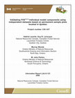
Ecological Modelling, 2004
Download

Download

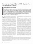
The Forestry Chronicle, 2008
Download

Ecological Modelling, 2013
Download

Ecological Applications, 2006
Download

The Forestry Chronicle, 2008
Download

Journal of Forestry, 2014
Download

Download

New Forests, 2015
Download

Ecological Modelling, 2001
Download
