Path Integral Bosonization of the ’t Hooft Determinant: Fluctuations and Multiple Vacua Alexander A. Osipov∗ and Brigitte Hiller arXiv:hep-ph/0204182v2 3 Jun 2002 Centro de Fı́sica Teórica, Departamento de Fı́sica da Universidade de Coimbra, 3004-516 Coimbra, Portugal (February 1, 2008) The ’t Hooft six quark flavor mixing interaction (Nf = 3) is bosonized by the path integral method. The considered complete Lagrangian is constructed on the basis of the combined ’t Hooft and U (3) × U (3) extended chiral four fermion Nambu – Jona-Lasinio interactions. The method of the steepest descents is used to derive the effective mesonic Lagrangian. Additionally to the known lowest order stationary phase (SP) result of Reinhardt and Alkofer we obtain the contribution from the small quantum fluctuations of bosonic configurations around their stationary phase trajectories. It affects the vacuum state of hadrons at low energies: whereas without the inclusion of quantum fluctuations the vacuum is uniquely defined for a fixed set of the model parameters, fluctuations give rise to multivalued solutions of the gap equations, marked at instances by drastic changes in the quark condensates. We derive the new gap equations and analyse them in comparison with known results. We classify the solutions according to the number of extrema they may accomodate. We find up to four solutions in the 0 < mu , ms < 3 GeV region. 12.39.Fe, 11.30.Rd, 11.30.Qc I. INTRODUCTION The global UL (3) × UR (3) chiral symmetry of the QCD Lagrangian (for massless quarks) is broken by the UA (1) Adler-Bell-Jackiw anomaly of the SU (3) singlet axial current q̄γµ γ5 q. Through the study of instantons [1,2], it has been realized that this anomaly has physical effects with the result that the theory contains neither a conserved U (1) quantum number, nor an extra Goldstone boson. Instead the effective 2Nf quark interactions arise, which are known as ’t Hooft interactions. In the case of two flavors they are four-fermion interactions, and the resulting low-energy theory resembles the old Nambu – Jona-Lasinio model [3]. In the case of three flavors they are six-fermion interactions which are responsible for the correct description of η and η ′ physics, and additionally lead to the OZI-violating effects [4,5], Ldet = κ(detq̄PR q + detq̄PL q) (1) where the matrices PR,L = (1 ± γ5 )/2 are projectors and determinant is over flavor indices. The physical degrees of freedom of QCD at low-energies are mesons. The bosonization of the effective quark interaction (1) by the path integral approach has been considered in [6], where the lowest order stationary phase approximation (SPA) has been used to estimate the leading contribution from the ’t Hooft determinant. In this approximation the functional integral is dominated by the stationary trajectories rst (x), determined by the extremum condition δS(r) = 0 of the action S(r). The lowest order SPA corresponds to the case in which the integrals associated with δ 2 S(r), for the path rst (x) are neglected and only S(rst ) contributes to the generating functional. The next natural step in this scenario is to complete the semiclassical result of Reinhardt and Alkofer by including the contribution from the integrals associated with the second functional derivative δ 2 S(rst ), and this is the subject of our paper. An alternative method of bosonizing the ’t Hooft determinant has been reviewed in [7]. The special path integral representation for the quark determinant has been obtained by considering Nc as an algebraically large parameter. One should not forget that the ’t Hooft’s determinant interactions are induced by instantons and only can be written in the simple determinantal form (1) in the limit of large number of colours – otherwise the many-fermion interactions have a more complicated structure. For our calculations it means, in particular, that the terms of the bosonized Lagrangian induced by the ’t Hooft’s determinant interaction (1) should be of order 1, corresponding to the standard rules of Nc counting. In this respect it is worthwhile to note that we have found that the meson vertices, induced by ∗ On leave from the Joint Institute for Nuclear Research, Laboratory of Nuclear Problems, 141980 Dubna, Moscow Region, Russia. 1 the ’t Hooft’s determinant interactions in the lowest order SPA and the term from the integral associated with the second functional derivative δ 2 S(rst ) have the same Nc -order and should be considered on the same footing. II. PATH INTEGRAL BOSONIZATION To be definite, let us consider the theory of the quark fields in four dimensional Minkowski space, with dynamics defined by the Lagrangian density L = LNJL + Ldet . (2) The first term here is the extended version of the Nambu – Jona-Lasinio (NJL) Lagrangian LNJL = L0 + Lint , consisting of the free field part L0 = q̄(iγ µ ∂µ − m̂)q, (3) and the U (3)L × U (3)R chiral symmetric four-quark interaction G Lint = [(q̄λa q)2 + (q̄iγ5 λa q)2 ]. 2 (4) We assume that quark fields have color and flavor indices running through the set i = 1, 2, 3; λa are the standard U (3) Gell-Mann matrices with a = 0, 1, . . . , 8. The current quark mass, m̂, is a nondegenerate diagonal matrix with elements diag(m̂u , m̂d , m̂s ), it explicitly breaks the global chiral U (3)L × U (3)R symmetry of the LNJL Lagrangian. The second term in (2) is given by (1). Letting sa = −q̄λa q, pa = q̄iγ5 λa q, s = sa λa , p = pa λa (5) yields κ Ldet = − [det(s + ip) + det(s − ip)] 64 (6) with determinants written in terms of the mesonic type quark bilinears. This identity is a first step to the bosonization of the theory with Lagrangian (2). The dynamics of the system is described by the vacuum transition amplitude in the form of the path integral  Z  Z 4 Z = DqDq̄ exp i d xL . (7) By means of a simple trick, suggested by Reinhardt and Alkofer, it is easy to write down this amplitude as   Z Z Z = DqDq̄Dσa Dφa Dr1a Dr2a exp i d4 xL′ (8) with L′ = q̄(iγ µ ∂µ − m̂ − σ + iγ5 φ)q − + r2a (φa − Gq̄iγ5 λa q) −  1  (σa )2 + (φa )2 + r1a (σa + Gq̄λa q) 2G κ [det(σ + iφ) + det(σ − iφ)] . (4G)3 (9) Eq.(8) defines the same expression as Eq.(7). To see this one has to integrate first over auxiliary fields r1a , r2a . It leads to δ-functionals which can be integrated out by taking integrals over σa , and φa , and which bring us back to the expression (7). From the other side, it is easy to rewrite Eq.(8) in a form appropriate to finish the bosonization, i.e., to calculate the integrals over quark fields and integrate out from Z the unphysical part of the auxiliary r1a , r2a scalar fields. Indeed, introducing new variables σ → σ + Gr1 , φ → φ + Gr2 , and after that r1 → 2r1 − σ/G, r2 → 2r2 − φ/G we have  Z Z  Z  Z Z = Dσa Dφa DqDq̄ exp i d4 xLq (q̄, q, σ, φ) Dr1a Dr2a exp i d4 xLr (σ, φ, r1 , r2 ) (10) 2 where Lq = q̄(iγ µ ∂µ − m̂ − σ + iγ5 φ)q,   κ Lr = 2G (r1a )2 + (r2a )2 − 2(r1a σa + r2a φa ) − [det(r1 + ir2 ) + det(r1 − ir2 )] . 8 (11) (12) The Fermi fields enter the action bilinearly, we can always integrate over them, because in this case we deal with the standard Gaussian type integral. At this stage one should also shift the scalar fields σa → σa + ∆a by demanding that the vacuum expectation values of the shifted fields vanish < 0|σa |0 >= 0. In other words, all tadpole graphs in the end should sum to zero, giving us gap equations to fix parameters ∆a . Here ∆a = ma − m̂a , with ma denoting the constituent quark masses 1 . To evaluate path integrals over r1,2 one has to use the method of stationary phase, or, after the formal analytic continuation in the time coordinate x4 = ix0 , the method of steepest descents. Let us consider this task in some detail. The Euclidean (imaginary time) version of the path integral under consideration is Z  Z +∞ J(σ, φ) = Dr1a Dr2a exp d4 xLr (σ, φ, r1 , r2 ) . (13) −∞ This integral is hopelessly divergent even if κ = 0. One should say at this point that we are not really interested in (13) but only in its analytic continuation. Let us suppose we analytically change Lr (σ, φ, r1 , r2 ) in some way such that we go from this situation back to the one of interest. To keep the integral convergent, we must distort the contour of integration into the complex plane following the standard procedure of the method of the steepest descents. This method gives the first term in an asymptotic expansion of J(σ, φ), valid for h̄ → 0. We lead the contour along the a straight line which is parallel to the imaginary axis and crosses the real axis at the saddle point rst . It is in the sense of this continuation that the integral J(σ, φ) of (13) is to be interpreted as J(σ, φ) = Z +i∞+r −i∞+r st st Dr1a Dr2a exp Z  d xLr (σ, φ, r1 , r2 ) . 4 (14) a , Near the saddle point rst Lr ≈ Lr (rst ) + 1X r̃α L′′αβ (rst )r̃β 2 (15) α,β a where the saddle point, rst , is a solution of the equations L′r (r1 , r2 ) = 0 determining a flat spot of the surface Lr (r1 , r2 ).  b c b c 2Gr1a − (σ + ∆)a − 3κ 8 Aabc (r1 r1 − r2 r2 ) = 0 (16) b c A r 2Gr2a − φa + 3κ abc 1 r2 = 0. 4 This system is well-known from [6]. The totally symmetric constants, Aabc , come from the definition of the flavor determinant: det r = Aabc ra rb rc , and equal to Aabc = 1 ǫijk ǫmnl (λa )im (λb )jn (λc )kl . 3! (17) a They are closely related with the U (3) constants dabc . We use in (15) symbols r̃a for the differences (ra − rst ). To a a deal with the multitude of integrals in (14) we define a column vector r̃ with eighteen components r̃α = (r̃1 , r̃2 ) and with the matrix L′′αβ (rst ) being equal to   3κ 3κ c Aabc r1cst δab − 8G 8G Aabc r2st . (18) L′′αβ (rst ) = 4GQαβ , Qαβ = 3κ 3κ c δab + 8G Aabc r1cst 8G Aabc r2st Eq.(14) can now be concisely written as 1 The shift by the current quark mass is needed to hit the correct vacuum state, see e.g. [8]. 3 Z J(σ, φ) = exp Z d4 xLr (rst ) +i∞ −i∞  Z  Dr̃α exp 2G d4 xr̃t Q(rst )r̃ [1 + O(h̄)] . (19) Our next task is to evaluate the integrals over r̃α . Before we do this, though, some comments should be made about what we have done so far: (1) The first exponential factor in Eq.(19) is not new. It has been obtained by Reinhardt and Alkofer in [6]. A bit of manipulation with expressions (12) and (16) leads us to the result Lr (rst ) = 2 G[(r1ast )2 + (r2ast )2 ] − 2[(σ + ∆)a r1ast + φa r2ast ] . 3 (20) One can try to solve Eqs.(16) looking for solutions r1ast and r2ast in the form of increasing powers in σa , φa (1) (1) (2) r1ast = ha + hab σb + habc σb σc + habc φb φc + . . . r2ast = (2) hab φb + (3) habc φb σc (21) + ... (22) Putting these expansions in Eqs.(16) one can obtain the series of selfconsistent equations to determine the constants (1) (2) ha , hab , and hab 3κ Aabc hb hc = 0, 2Gha − ∆a − 8   3κ 2G δac − Aacb hb h(1) ce = δae , 8G   3κ 2G δac + Aacb hb h(2) ce = δae . 8G (23) (24) (25) The other constants can be obtained from these ones, for instance, we have (1) habc = 3κ (1) (1) (1) h h h A , 8 aā bb̄ cc̄ āb̄c̄ (2) habc = − 3κ (1) (2) (2) h h h A , 8 aā bb̄ cc̄ āb̄c̄ (3) habc = − 3κ (2) (2) (1) h h h A . 4 aā bb̄ cc̄ āb̄c̄ (26) As a result the effective Lagrangian (20) can be expanded in powers of meson fields. Such an expansion (up to the terms which are cubic in σa , φa ) looks like (1) (2) Lr (rst ) = −2ha σa − hab σa σb − hab φa φb + O(field3 ). (27) (2) Our result (19) has been based on the assumption that all eigenvalues of matrix Q are positive. It is true, for instance, if κ = 0. It may happen, however, that some eigenvalues of Q are negative for some range of parameters G and κ. In these cases there are no conceptual difficulties, for from the very beginning we deal with well defined Gaussian integrals and the integration over the corresponding r̃α simply does not require analytic continuation. We now turn to the evaluation of the path integral in Eq.(19). In order to define the measure Dr̃α more accurately let us expand r̃α in a Fourier series r̃α (x) = ∞ X cn,α ϕn (x), (28) n=1 assuming that suitable boundary conditions are imposed. The set of the real functions {ϕn (x)} form an orthonormal and complete sequence Z d4 xϕn (x)ϕm (x) = δnm , ∞ X n=1 ϕn (x)ϕn (y) = δ(x − y). (29) Therefore Z  Z  Z n X o C Dr̃α exp 2G d4 xr̃t Q(rst )r̃ = dcn,α exp 2G cn,α λαβ . nm cm,β = q det(2Gλαβ ) nm The normalization constant C is not important for the following. The matrix λαβ nm is equal to 4 (30) λαβ nm = Z d4 xϕn (x)Qαβ (x)ϕm (x). (31) From (18) and (29) it follows that 2Gλαβ nm (1)−1 hac 0 = 0 (2)−1 hac ! ασ   Z δσβ δnm + d4 xϕn (x)Fσβ (x)ϕm (x) (32) with Fσβ 3κ Aeba = 4 (1) (1) −hce (r1ast − ha ) hce r2ast (2) a (2) a hce r2st hce (r1st − ha ) ! . (33) σβ Only the matrix Fσβ depends here on fields σ, φ. By absorbing in C the irrelevant field independent part of 2Gλαβ nm , and expanding the logarithm in the representation det(1 + F ) = exp tr ln(1 + F ), one can obtain finally for the integral in (19) ( ) Z ∞ ∞ X 1 X (−1)n  n 4 ′ Sr J(σ, φ) = C e , Sr = d x Lr (rst ) + tr Fαβ (rst ) ϕm (x)ϕm (x) . (34) 2 n n=1 m=1 The sum over m in this expression, however, is not well defined and needs to be regularized. One can regularize it by introducing a Gaussian cutoff M damping the contributions from the large momenta k 2 ∞ X m=1 ϕm (x)ϕm (x) = δ(0) ∼ Z   M4 d4 k k2 = exp − (2π)4 M2 16π 2 ∞ −∞ (35) This procedure does not decrease the predictability of the model, for anyway one has to regularize the quark loop contributions in (10). Alternatively, following ideas presented in [9], one can introduce the Ansatz: ( ) Z ∞  a X (−1)n  n 4 Sr = d x Lr (rst ) + (36) tr Fαβ (rst ) 2G2 n n=1 proposing that the undetermined dimensionless constant a will be fixed by confronting the model with experiment afterwards. III. THE GROUND STATE Let us study the ground state of the model under consideration, then properties of the excitations will follow naturally. To make further progress let us note that Eqs.(23) have non-trivial solutions for h0 , h3 , h8 , corresponding to the spontaneous breaking of chiral symmetry in the physical vacuum state with order parameters ∆i 6= 0 (i = u, d, s). We may then use this fact to rewrite Eqs.(23) as a system of only three equations to give hi 2Ghi − ∆i = κ tijk hj hk 8 (37) where the totally symmetric coefficients tijk are equal to zero except for tuds = 1. 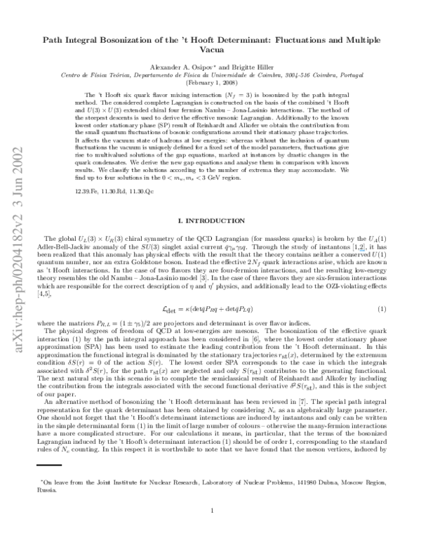They are related to coefficients Aabc by the embedding formula 3ωia Aabc ebj eck = tijk where matrices ωia , and eai are defined as follows 5 2000 14 12 0 k GeV-5 G GeV-2 10 8 -2000 6 -4000 4 2 0 0.1 0.2 0.3 mu GeV 0 0.4 0.1 enter text here 0.2 mu GeV 0.3 0.4 FIG. 1. The couplings G (left panel) and κ (right panel) as functions of mu at fixed values of ms = 572 MeV and other parameters in Eq.(41). These curves show the typical mu -dependence of the functions if one neglects the fluctuations term in Eq.(39). eai √ √ √  2 1  √2 √2 = √ 3 − 3 0 , 2 3 1 1 −2 ωia √ √  2 √3 1 1 √ = √ 2 − 3 1 . 3 √2 0 −2 (38) Here the index a runs a = 0, 3, 8 (for the other values of a the corresponding matrix elements are equal to zero). We have also ha = eai hi , and hi = ωia ha . Similar relations can be obtained for ∆i and ∆a . In accordance with these (1) (1) notations we will use, for instance, that hci = ωia hca . A tadpole graphs calculation gives for the gap equations the following result 2hi +  3aκ  (2) Nc (1) (1) h − h mi J0 (m2i ) ab ab Aabc hci = 2 8G 2π 2 (39) where the left hand side is the contribution from (36) and the right hand side is the contribution of the quark loop from (10) with a regularized quadratically divergent integral J0 (m2 ) being defined as Z ∞ dt −tm2 J0 (m2 ) = e ρ(t, Λ2 ), ρ(t, Λ2 ) = 1 − (1 + tΛ2 ) exp(−tΛ2 ). (40) t2 0 14 800 12 c 600 c 400 10 GeV-5 8 d 200 0 k G GeV-2 b a -200 6 d -400 4 0.26 0.26 a b -600 0.28 0.3 0.32 mu GeV 0.34 0.28 0.3 0.32 mu GeV 0.34 FIG. 2. The couplings G (left panel) and κ (right panel) as functions of mu for the same (as in Fig.1) values of other fixed parameters and for the case when the fluctuations term in Eq.(39) is taken into account. 6 c 800 12 c 10 D 600 b A D 6 d 4 k GeV-5 G GeV-2 400 8 B a E 200 d 0 a -200 C C A E -400 2 B -600 0 0.25 0.5 0.75 mu GeV 1 1.25 b 0 1.5 0.25 0.5 0.75 mu GeV 1 1.25 1.5 FIG. 3. Different classes of mu solutions of the gap equations, including fluctuations, at fixed G, κ values. Four branches of solutions, A, B, C and a − b stretch have negative κ. Three branches, D, E and along c − d arm correspond to positive κ. Bold dashes indicate that only one solution exists in this region of G, κ. See further details in text. The second term on the left hand side of Eq.(39) is the correction resulting from the Gaussian integrals of the steepest descent method, comprising the effects of small fluctuations around the stationary path. If one puts for a moment a = 0 in Eq.(39), and combines the result with Eqs.(37), one finds gap equations which are very similar to the ones obtained in [4] (see equation (2.12) therein). At fixed input parameters G, κ, Λ of the model, the gap equations can be solved giving us the constituent quark masses mi as functions of the current quark masses, mi = mi (m̂j ). Alternatively, by fixing m̂i , one can obtain from the gap equations the non-trivial solutions mi = mi (G, κ, Λ). In particular, when m̂u = m̂d , these equations can be solved for G and κ, giving expressions  2  2 2 2π mu ∆u J0 (m2u ) − ms ∆s J0 (m2s ) ms ∆u J0 (m2s ) − mu ∆s J0 (m2u ) 8π G= , κ = . (41) 2 2 Nc m2u J0 (m2u ) − m2s J0 (m2s ) Nc mu J0 (m2u )[m2u J02 (m2u ) − m2s J02 (m2s )] In Fig.1 we plot the curves of G and κ versus mu keeping constant Λ = 0.87 GeV, ms = 572 MeV, m̂s = 200 MeV, m̂u = 6 MeV. One can readily see that at given values for (mu , ms ) the curves yield unique values of (G, κ), i.e. the vacuum state is well-defined in this case. 800 12 600 10 D B 6 D E k GeV-5 G GeV-2 400 8 A E 200 0 A C -200 4 C -400 2 B -600 0 0.25 0.5 0.75 1 ms GeV 1.25 1.5 0 0.5 1 1.5 ms GeV 2 2.5 3 FIG. 4. The same as in figure 3 for the ms solutions. The dashes are the constant ms corresponding to the abcd curve of Figs. 2 and 3. Let us consider now the general case which we have when a > 0 in Eq.(39). To illustrate the qualitative difference with the previous case we put for definiteness a = 1 and look again for the solutions G = G(mu ) and κ = κ(mu ) with the same set of fixed parameters. The corresponding curves are plotted in Fig.2. If the mass mu is sufficiently (min) low that mu < mu , (in the figures denoted by the region left the turning point c) or sufficiently high that (max) mu < mu < ms , (in the figures denoted by the region right to the turning point b), then there exists again a 7 (min) (max) , < mu < mu single solution with unique values of (G, κ). However, there is now a region for mu in which mu where three values of couplings (G, κ) are possible. Conversely, one can study the solutions: mu = mu (G, κ), ms = ms (G, κ at fixed values of input parameters: Λ, m̂u = m̂d , m̂s ). As starting input values for the couplings G and κ in the gap equations we take the ones already determined along the path abcd shown in Fig.2, obtained at a constant value of the strange quark mass, ms = 572 MeV. For a chosen value of the set (G, κ) we then search for further solutions (mu , ms ) of the Eq.(39), displaying results in Fig.3 for mu and in Fig.4 for ms , correspondingly. The dashed curves are the repetition of the solutions encountered in Fig.2. The bold dashes in Fig.3 indicate that we only find this one solution at fixed values of G, κ. Combining the information of Figs.3 and 4, one sees that one has up to four solutions at fixed G, κ. Indeed, travelling along the original path abcd one observes the following: the branch ab is accompanied by three other branches, marked as A, B and C which belong to the same class of solutions. One sees that these solutions have negative κ values. From the turning point b until the maximum value of G (and corresponding κ) (bold dashes) we have no other solutions to the gap equations, as already stated. From this maximum G value to the turning point c and further along the cd arm we encounter further two branches, denoted by D and E to the solutions of Eqs.(39) with same G, κ. They are positive κ solutions. This very rich structure of the vacuum solutions implies the possibility of having several different values of the quark condensates for the same G, κ parameters, embracing also the possibility which has been considered in connection with generalized chiral perturbation theory (see e.g. section 4 in [10]). We give here only a few examples. At G = 4.54 GeV−2 , κ = 153.04 GeV−5 we have three solutions. The solution mu = 346 MeV, ms = 572 MeV, on the cd arm has the quark condensates < ūu >1/3 = −236.8 MeV, < s̄s >1/3 = −183.5 MeV and the ratio R = (< s̄s > / < ūu >)1/3 = 0.775; the second solution, on the E branch with mu = 535 MeV, ms = 732 MeV has condensates < ūu >1/3 = −249 MeV, < s̄s >1/3 = −183 MeV and the ratio R = 0.738; the third solution, located at the D branch with mu = 46 MeV, ms = 418 MeV has condensates < ūu >1/3 = −131 MeV, < s̄s >1/3 = −172 MeV and R = 1.313. We chose the next example at G = 8.126 GeV−2 , κ = −544.81 GeV−5 , where there are four solutions. The solution mu = 316 MeV, ms = 572 MeV, on the ab arm has the quark condensates < ūu >1/3 = −233 MeV, < s̄s >1/3 = −184 MeV and R = 0.787; the second solution, on the B branch with mu = 624 MeV, ms = 205 MeV has condensates < ūu >1/3 = −249 MeV, < s̄s >1/3 = −56.7 MeV and R = 0.227; the third solution, located at the A branch with mu = 421 MeV, ms = 1.84 GeV has condensates < ūu >1/3 = −14.4 MeV, < s̄s >1/3 = −86 MeV and R = 0.353. The fourth solution, on the C branch, with mu = 1.394 GeV, ms = 1.594 GeV has condensates < ūu >1/3 = −230 MeV, < s̄s >1/3 = −120 MeV and the ratio R = 0.524. As a final example we take the solutions at G = 11.96 GeV−2 ≃ Gmax , κ = 371.491 GeV−5 , where the branches D and E emerge and are very close to each other with mu = 1.56 GeV, ms = 1.72 GeV. The corresponding condensates are < ūu >1/3 = −224 MeV, < s̄s >1/3 = −105 MeV and R = 0.467. The other solution is at the path bc with mu = 290 MeV, ms = 572 MeV with condensates < ūu >1/3 = −229 MeV, < s̄s >1/3 = −184 MeV and R = 0.8. To summarize, we have found that in the presence of the ’t Hooft interaction, treated beyound the lowest order SPA, several solutions to the gap equations are possible at some range of input parameters, i.e. the same values of G, κ, Λ, m̂i lead to different sets of constituent quark masses (mu , ms ) and, therefore, to different values of the quark condensates. A quite different scenario emerges for the hadronic vacuum, which can now be multivalued. It makes our result essentially different from the ones obtained in [6,4]. These findings must be further analysed in order to establish which of the extrema correspond to minima or maxima of the effective potential. This step will be done elsewhere in conjunction with the determination of the meson mass spectrum, as it also requires dealing with the terms with two powers of the meson fields in the ansatz of solutions Eq.(21) and in the related Lagrangian (27). IV. CONCLUDING REMARKS The purpose of this work has been twofold. Firstly we have developed the technique which is necessary to go beyound the lowest order SPA in the problem of the path integral bosonization of the ’t Hooft six quark interaction. We have shown how the pre-exponential factor, connected with the steepest descent approach and which is responsible for the quantum fluctuations around the classical path, can be treated exactly, order by order, in a scheme of increasing number of mesonic fields, while preserving all chiral symmetry requirements. This technique is rather general and can be readily used in other applications. Second, we have explored with considerable detail the implications of taking the quantum fluctuations in account in the description of the hadronic vacuum. A very complex multivalued vacuum emerges at fixed values of the input parameters G, κ, Λ and current quark masses. We encountered several classes of solutions. Searching in an interval of constituent quark masses from zero to ≃ 3GeV, we found G, κ, regions caracterized by one, three and four solutions. The multiple vacua may have very interesting physical consequences and applications. 8 ACKNOWLEDGEMENTS We are grateful to Dmitri Diakonov for valuable correspondence. We thank Dmitri Osipov and Pedro Costa for their help in converting the “Mathematica” generated figures into the final ones. This work is supported by grants provided by Fundação para a Ciência e a Tecnologia, POCTI/35304/FIS/2000 and NATO ”Outreach” Cooperation Program. [1] A. M. Polyakov, Phys. Lett. B 59 (1975) 82; Nucl. Phys. B 121 (1977) 429. A. A. Belavin, A. M. Polyakov, A. Schwartz and Y. Tyupkin, Phys. Lett. B 59 (1975) 85. G. ’t Hooft, Phys. Rev. Lett. 37 (1976) 8; Phys. Rev. D 14 (1976) 3432. C. Callan, R. Dashen and D. J. Gross, Phys. Lett. B 63 (1976) 334. R. Jackiw and C. Rebbi, Phys. Rev. Lett. 37 (1976) 172. S. Coleman, “The uses of instantons” Erice Lectures, 1977. [2] D. Diakonov, “Chiral symmetry breaking by instantons”, Lectures at the Enrico Fermi School in Physics, Varenna, June 27 - July 7 (1995); hep-ph/9602375. [3] Y. Nambu, G. Jona-Lasinio, Phys. Rev. 122 (1961) 345; 124 (1961) 246; V. G. Vaks, A. I. Larkin ZhETF 40 (1961) 282. [4] V. Bernard, R. L. Jaffe, U.-G. Meißner, Nucl. Phys. B 308 (1988) 753. [5] T. Kunihiro and T. Hatsuda, Phys. Lett. B 206 (1988) 385. T. Hatsuda, Phys. Lett. B 213 (1988) 361. Y. Kohyama, K. Kubodera and M. Takizawa, Phys. Lett. B 208 (1988) 165. M. Takizawa, Y. Kohyama and K. Kubodera, Prog. Theor. Phys. 82 (1989) 481. [6] H. Reinhardt and R. Alkofer, Phys. Lett. B 207 (1988) 482. [7] D. Diakonov, “Chiral quark-soliton model”, Lectures at the Advanced Summer School on non-perturbative field theory, Peniscola, Spain, June 2-6 (1997); hep-ph/9802298. [8] A.A. Osipov and B. Hiller, Phys. Rev. D 62 (2000) 114013; idem Phys. Rev. D 63 (2001) 094009. [9] R. Jackiw, Int. J. Mod. Phys. B 14 (2000) 2011; hep-th/9903044. [10] H. Leutwyler, Talk given at the Conf. on Fundamental Interactions of Elem. Part., ITEP, Moscow, Russia, 1995, CERNTH/96-25; hep-ph/9602255. 9 Path Integral Bosonization of the 't Hooft Determinant: Flu tuations and Multiple Va ua Alexander A. Osipov and Brigitte Hiller Centro de F si a Te ori a, Departamento de F si a da Universidade de Coimbra, 3004-516 Coimbra, Portugal (May 29, 2002) The 't Hooft six quark avor mixing intera tion (Nf = 3) is bosonized by the path integral method. The onsidered omplete Lagrangian is onstru ted on the basis of the ombined 't Hooft and U (3)  U (3) extended hiral four fermion Nambu { Jona-Lasinio intera tions. The method of the steepest des ents is used to derive the e e tive mesoni Lagrangian. Additionally to the known lowest order stationary phase (SP) result of Reinhardt and Alkofer we obtain the ontribution from the small quantum u tuations of bosoni on gurations around their stationary phase traje tories. It a e ts the va uum state of hadrons at low energies: whereas without the in lusion of quantum u tuations the va uum is uniquely de ned for a xed set of the model parameters, u tuations give rise to multivalued solutions of the gap equations, marked at instan es by drasti hanges in the quark ondensates. We derive the new gap equations and analyse them in omparison with known results. We lassify the solutions a ording to the number of extrema they may a omodate. We nd up to four solutions in the 0 < mu ; ms < 3 GeV region. 12.39.Fe, 11.30.Rd, 11.30.Q I. INTRODUCTION The global UL (3)  UR (3) hiral symmetry of the QCD Lagrangian (for massless quarks) is broken by the UA (1) Adler-Bell-Ja kiw anomaly of the SU (3) singlet axial urrent q  5 q . Through the study of instantons [1,2℄, it has been realized that this anomaly has physi al e e ts with the result that the theory ontains neither a onserved U (1) quantum number, nor an extra Goldstone boson. Instead the e e tive 2Nf quark intera tions arise, whi h are known as 't Hooft intera tions. In the ase of two avors they are four-fermion intera tions, and the resulting low-energy theory resembles the old Nambu { Jona-Lasinio model [3℄. In the ase of three avors they are six-fermion intera tions whi h are responsible for the orre t des ription of  and  0 physi s, and additionally lead to the OZI-violating e e ts [4,5℄, Ldet = (detqPR q + detqPL q) (1) where the matri es PR;L = (1  5 )=2 are proje tors and determinant is over avor indi es. The physi al degrees of freedom of QCD at low-energies are mesons. The bosonization of the e e tive quark intera tion (1) by the path integral approa h has been onsidered in [6℄, where the lowest order stationary phase approximation (SPA) has been used to estimate the leading ontribution from the 't Hooft determinant. In this approximation the fun tional integral is dominated by the stationary traje tories rst (x), determined by the extremum ondition ÆS (r) = 0 of the a tion S (r). The lowest order SPA orresponds to the ase in whi h the integrals asso iated with Æ 2 S (r), for the path rst (x) are negle ted and only S (rst ) ontributes to the generating fun tional. The next natural step in this s enario is to omplete the semi lassi al result of Reinhardt and Alkofer by in luding the ontribution from the integrals asso iated with the se ond fun tional derivative Æ 2 S (rst ), and this is the subje t of our paper. An alternative method of bosonizing the 't Hooft determinant has been reviewed in [7℄. The spe ial path integral representation for the quark determinant has been obtained by onsidering N as an algebrai ally large parameter. One should not forget that the 't Hooft's determinant intera tions are indu ed by instantons and only an be written in the simple determinantal form (1) in the limit of large number of olours { otherwise the many-fermion intera tions have a more ompli ated stru ture. For our al ulations it means, in parti ular, that the terms of the bosonized Lagrangian indu ed by the 't Hooft's determinant intera tion (1) should be of order 1, orresponding to the standard rules of N ounting. In this respe t it is worthwhile to note that we have found that the meson verti es, indu ed by  On leave from the Joint Institute for Nu lear Resear h, Laboratory of Nu lear Problems, 141980 Dubna, Mos ow Region, Russia. 1 the 't Hooft's determinant intera tions in the lowest order SPA and the term from the integral asso iated with the se ond fun tional derivative Æ 2 S (rst ) have the same N -order and should be onsidered on the same footing. II. PATH INTEGRAL BOSONIZATION To be de nite, let us onsider the theory of the quark elds in four dimensional Minkowski spa e, with dynami s de ned by the Lagrangian density L = LNJL + Ldet : (2) The rst term here is the extended version of the Nambu { Jona-Lasinio (NJL) Lagrangian LNJL = onsisting of the free eld part L0 = q(i  L0 + Lint , m ^ )q;  (3) and the U (3)L  U (3)R hiral symmetri four-quark intera tion Lint = G2 [(qa q)2 + (qi 5 a q ) 2 ℄: (4) We assume that quark elds have olor and avor indi es running through the set i = 1; 2; 3; a are the standard U (3) Gell-Mann matri es with a = 0; 1; : : : ; 8. The urrent quark mass, m ^ , is a nondegenerate diagonal matrix with elements diag(m ^ u; m ^ d; m ^ s ), it expli itly breaks the global hiral U (3)L  U (3)R symmetry of the LNJL Lagrangian. The se ond term in (2) is given by (1). Letting sa = qa q; pa = qi 5 a q; s = sa a ; p = pa a (5) yields  Ldet = 64 [det(s + ip) + det(s ip)℄ (6) with determinants written in terms of the mesoni type quark bilinears. This identity is a rst step to the bosonization of the theory with Lagrangian (2). The dynami s of the system is des ribed by the va uum transition amplitude in the form of the path integral Z Z= DqDq exp  Z i  d xL : 4 (7) By means of a simple tri k, suggested by Reinhardt and Alkofer, it is easy to write down this amplitude as Z Z= DqDqDa Da Dr1a Dr2a exp  Z i d4 xL0  (8) with L 0 = q(i   + r2a (a 1   ( )2 + (a )2 + r1a (a + Gqa q )  + i 5 )q 2G a  Gqi 5 a q ) [det( + i) + det( i)℄ : (4G)3 m ^ (9) Eq.(8) de nes the same expression as Eq.(7). To see this one has to integrate rst over auxiliary elds r1a ; r2a . It leads to Æ -fun tionals whi h an be integrated out by taking integrals over a , and a , and whi h bring us ba k to the expression (7). From the other side, it is easy to rewrite Eq.(8) in a form appropriate to nish the bosonization, i.e., to al ulate the integrals over quark elds and integrate out from Z the unphysi al part of the auxiliary r1a ; r2a s alar elds. Indeed, introdu ing new variables  !  + Gr1 ;  !  + Gr2 , and after that r1 ! 2r1 =G; r2 ! 2r2 =G we have Z Z= Da Da DqDq exp  Z i d4 xLq ( q ; q; ; ) Z 2 Dr1a Dr2a exp  Z i d4 xLr (; ; r1 ; r2 )  (10) where Lq = q(i   m^  + i 5 )q;   Lr = 2G (r1a )2 + (r2a )2 2(r1a a + r2a a ) 8 [det(r1 + ir2 ) + det(r1 (11) ir2 )℄ : (12) The Fermi elds enter the a tion bilinearly, we an always integrate over them, be ause in this ase we deal with the standard Gaussian type integral. At this stage one should also shift the s alar elds a ! a +
a by demanding that the va uum expe tation values of the shifted elds vanish < 0jaj0 >= 0. In other words, all tadpole graphs in the end should sum to zero, giving us gap equations to x parameters
a. Here
a = ma m^ a , with ma denoting the onstituent quark masses 1. To evaluate path integrals over r1;2 one has to use the method of stationary phase, or, after the formal analyti ontinuation in the time oordinate x4 = ix0 , the method of steepest des ents. Let us onsider this task in some detail. The Eu lidean (imaginary time) version of the path integral under onsideration is ( )= J ;  Z +1 1 Dr1a Dr2a exp Z ( d4 xLr ; ; r1 ; r2 )  : (13) This integral is hopelessly divergent even if  = 0. One should say at this point that we are not really interested in (13) but only in its analyti ontinuation. Let us suppose we analyti ally hange Lr (; ; r1 ; r2) in some way su h that we go from this situation ba k to the one of interest. To keep the integral onvergent, we must distort the ontour of integration into the omplex plane following the standard pro edure of the method of the steepest des ents. This method gives the rst term in an asymptoti expansion of J (; ), valid for h ! 0. We lead the ontour along the straight line whi h is parallel to the imaginary axis and rosses the real axis at the saddle point rsta . It is in the sense of this ontinuation that the integral J (; ) of (13) is to be interpreted as Z  Z +i1+r st 4 Dr1a Dr2a exp d xLr (; ; r1 ; r2 ) : J (; ) = (14) i1+rst Near the saddle point rsta , X Lr  Lr (rst ) + 21 r~ L00 (rst )~r (15) ; where the saddle point, rsta , is a solution of the equations L0r (r1 ; r2 ) = 0 determining a at spot of the surfa e Lr (r1 ; r2 ).  2Gr1a ( +
)a 38 Aab (r1b3r1 r2bbr2) = 0 (16) 2Gr2a a + 4 Aab r1 r2 = 0: This system is well-known from [6℄. The totally symmetri onstants, Aab , ome from the de nition of the avor determinant: det r = Aab rarb r , and equal to 1 Aab = ijk mnl (a )im (b )jn ( )kl : (17) 3! They are losely related with the U (3) onstants dab . We use in (15) symbols r~a for the di eren es (ra rsta ). To deal with the multitude of integrals in (14) we de ne a olumn ve tor r~ with eighteen omponents r~ = (~r1a ; r~2a ) and 00 with the matrix L (rst ) being equal to   A r 3 Aab r Æab 83G ab 00 8 G 1 st 2 st : (18) L (rst ) = 4GQ ; Q = A r 3 Æab + 83G ab 1st 8G Aab r2st Eq.(14) an now be on isely written as 1 The shift by the urrent quark mass is needed to hit the orre t va uum state, see e.g. [8℄. 3 Z  Z +i1  Z  ~t ( st )~r [1 + O(h)℄ : (19) i1 Our next task is to evaluate the integrals over r~ . Before we do this, though, some omments should be made about what we have done so far: (1) The rst exponential fa tor in Eq.(19) is not new. It has been obtained by Reinhardt and Alkofer in [6℄. A bit of manipulation with expressions (12) and (16) leads us to the result  (20) Lr (rst ) = 32 G[(r1ast )2 + (r2ast )2 ℄ 2[( +
)a r1ast + a r2ast ℄ : One an try to solve Eqs.(16) looking for solutions r1ast and r2ast in the form of in reasing powers in a; a (1) (1) (2) r1ast = ha + hab b + hab b  + hab b  + : : : (21) (2) (3) a r2st = hab b + hab b  + : : : (22) Putting these expansions in Eqs.(16) one an obtain the series of self onsistent equations to determine the onstants (1) (2) ha , hab , and hab (23) 2Gha
a 38 Aab hb h = 0;   (24) 2G Æa 83G Aa b hb h(1)e = Æae ;   2G Æa + 83G Aa b hb h(2)e = Æae : (25) The other onstants an be obtained from these ones, for instan e, we have 3 h(1)h(1)h(1)A  ; h(2) = 3 h(1)h(2)h(2)A  ; h(3) = 3 h(2)h(2)h(1)A  : (1) (26) hab = 8 aa bb  ab ab 8 aa bb  ab ab 4 aa bb  ab As a result the e e tive Lagrangian (20) an be expanded in powers of meson elds. Su h an expansion (up to the terms whi h are ubi in a ; a) looks like (2) 3 Lr (rst ) = 2haa h(1) (27) ab a b hab a b + O( eld ): (2) Our result (19) has been based on the assumption that all eigenvalues of matrix Q are positive. It is true, for instan e, if  = 0. It may happen, however, that some eigenvalues of Q are negative for some range of parameters G and . In these ases there are no on eptual diÆ ulties, for from the very beginning we deal with well de ned Gaussian integrals and the integration over the orresponding r~ simply does not require analyti ontinuation. We now turn to the evaluation of the path integral in Eq.(19). In order to de ne the measure Dr~ more a urately let us expand r~ in a Fourier series ( ) = exp J ;  L ( st ) d4 x r r ~ (x) = r Dr~ exp 2G 1 X n=1 d4 xr Q r () (28) n; 'n x ; assuming that suitable boundary onditions are imposed. The set of the real fun tions f'n(x)g form an orthonormal and omplete sequen e Z Therefore Z  Dr~ exp 2G Z ( ) ( ) = Ænm; d4 x'n x 'm x  ~t ( st)~r = d4 xr Q r Z d n; 1 X n=1 ( ) ( ) = Æ(x 'n x ' n y n exp 2G X n; nm m; ) (29) y : o =q C det(2Gnm) The normalization onstant C is not important for the following. The matrix nm is equal to 4 : (30) nm = Z () d4 x'n x Q (x)'m (x): (31) From (18) and (29) it follows that 2Gnm = (1) 1 ha 0 0 (2) 1 ha with = 34 Aeba !   Æ Ænm + Z () d4 x'n x F (x)'m (x)  (32) ! ( st ha) h e rast : (33) F h e (rast ha ) st  Only the matrix F depends here on elds ; . By absorbing in C the irrelevant eld independent part of 2Gnm, and expanding the logarithm in the representation det(1+ F ) = exp trln(1+ F ), one an obtain nally for the integral in (19) ( ) Z 1 ( 1)n  1 X X 1 0 S n r d x Lr (rst ) + J (; ) = C e ; Sr = (34) 2 n n tr F (rst ) m 'm (x)'m (x) : The sum over m in this expression, however, is not well de ned and needs to be regularized. One an regularize it by introdu ing a Gaussian uto M damping the ontributions from the large momenta k h e r1a (2) h e r2a (1) (1) 2 (2) 1 4 =1 =1 2 1 X Z 1 d4 k  k2  4 M = exp (35) M 16 1 (2) m This pro edure does not de rease the predi tability of the model, for anyway one has to regularize the quark loop ontributions in (10). Alternatively, following ideas presented in [9℄, one an introdu e the Ansatz: ( ) Z 1  a X ( 1)n  n Sr = d x Lr (rst ) + (36) 2G n n tr F (rst ) proposing that the undetermined dimensionless onstant a will be xed by onfronting the model with experiment afterwards. =1 ( ) ( ) = Æ(0)  'm x ' m x 4 2 2 4 2 =1 III. THE GROUND STATE Let us study the ground state of the model under onsideration, then properties of the ex itations will follow naturally. To make further progress let us note that Eqs.(23) have non-trivial solutions for h ; h ; h , orresponding to the spontaneous breaking of hiral symmetry in the physi al va uum state with order parameters
i 6= 0 (i = u; d; s). We may then use this fa t to rewrite Eqs.(23) as a system of only three equations to give hi 2Ghi
i = 8 tijk hj hk (37) where the totally symmetri oeÆ ients tijk are equal to zero ex ept for tuds = 1. They are related to oeÆ ients Aab by the embedding formula 3!ia Aab ebj e k = tijk where matri es !ia , and eai are de ned as follows 0 5 3 8 2000 14 12 0 k GeV-5 G GeV-2 10 8 -2000 6 -4000 4 2 0 0.1 0.2 0.3 mu GeV 0 0.4 0.1 enter text here 0.2 mu GeV 0.3 0.4 FIG. 1. The ouplings G (left panel) and  (right panel) as fun tions of mu at xed values of ms = 572 MeV and other parameters in Eq.(41). These urves show the typi al mu -dependen e of the fun tions if one negle ts the u tuations term in Eq.(39). 1 eai = p 2 3 0p 2  p3 0p 2  p2 p p 1 p2 2 A ; p p3 1 1 1 !ia = p (38) 3 1 A: 3 0 p 3 1 1 2 2 0 2 Here the index a runs a = 0; 3; 8 (for the other values of a the orresponding matrix elements are equal to zero). We have also ha = eaihi , and hi = !iaha. Similar relations an be obtained for
i and
a. In a ordan e with these notations we will use, for instan e, that h i = !ia h a . A tadpole graphs al ulation gives for the gap equations the following result   2hi + 83Ga hab hab Aab h i = 2N mi J (mi ) (39) where the left hand side is the ontribution from (36) and the right hand side is the ontribution of the quark loop from (10) with a regularized quadrati ally divergent integral J (m ) being de ned as (1) (1) (2) (1) (1) 2 J0 (m2 ) = Z1 dt e t2 0 2 0 tm2  (t;  ); 2 2 0 2 (t; 2 ) = 1 (1 + t ) exp( t ): 2 (40) 2 14 800 12 c 600 c 400 10 GeV-5 8 d 200 0 k G GeV-2 b a -200 6 d -400 4 0.26 0.26 a b -600 0.28 0.3 0.32 mu GeV 0.34 0.28 0.3 0.32 mu GeV 0.34 FIG. 2. The ouplings G (left panel) and  (right panel) as fun tions of mu for the same (as in Fig.1) values of other xed parameters and for the ase when the u tuations term in Eq.(39) is taken into a ount. 6 c 800 12 c 10 D 600 b A D 6 d 4 k GeV-5 G GeV-2 400 8 B 200 d 0 a -200 C a E C A E -400 2 B -600 0 0.25 0.5 0.75 mu GeV 1 1.25 b 0 1.5 0.25 0.5 0.75 mu GeV 1 1.25 1.5 FIG. 3. Di erent lasses of mu solutions of the gap equations, in luding u tuations, at xed G;  values. Four bran hes of solutions, A; B; C and a b stret h have negative . Three bran hes, D; E and along d arm orrespond to positive . Bold dashes indi ate that only one solution exists in this region of G; . See further details in text. The se ond term on the left hand side of Eq.(39) is the orre tion resulting from the Gaussian integrals of the steepest des ent method, omprising the e e ts of small u tuations around the stationary path. If one puts for a moment a = 0 in Eq.(39), and ombines the result with Eqs.(37), one nds gap equations whi h are very similar to the ones obtained in [4℄ (see equation (2.12) therein). At xed input parameters G; ;  of the model, the gap equations an be solved giving us the onstituent quark masses mi as fun tions of the urrent quark masses, mi = mi (m^ j ). Alternatively, by xing m^ i, one an obtain from the gap equations the non-trivial solutions mi = mi (G; ; ). In parti ular, when m^ u = m^ d, these equations an be solved for G and , giving expressions  2   8  m
J (m ) m
J (m ) mu
u J (mu ) ms
s J (ms ) s u u s s u G= ; = : (41) N mu J (mu ) ms J (ms ) N mu J (mu )[mu J (mu ) ms J (ms )℄ In Fig.1 we plot the urves of G and  versus mu keeping onstant  = 0:87 GeV; ms = 572 MeV; m^ s = 200 MeV; m^ u = 6 MeV. One an readily see that at given values for (mu ; ms) the urves yield unique values of (G; ), i.e. the va uum state is well-de ned in this ase. 2 2 0 2 0 2 2 2 0 2 2 0 2 2 2 0 2 0 2 2 2 0 0 2 2 2 2 0 2 800 12 600 10 D B 6 D E k GeV-5 G GeV-2 400 8 A E 200 0 A C -200 4 C -400 2 B -600 0 0.25 0.5 0.75 1 ms GeV 1.25 1.5 0 0.5 1 1.5 ms GeV 2 2.5 3 FIG. 4. The same as in gure 3 for the ms solutions. The dashes are the onstant ms orresponding to the ab d urve of Figs. 2 and 3. Let us onsider now the general ase whi h we have when a > 0 in Eq.(39). To illustrate the qualitative di eren e with the previous ase we put for de niteness a = 1 and look again for the solutions G = G(mu ) and  = (mu ) with the same set ofminxed parameters. The orresponding urves are plotted in Fig.2. If the mass mu is suÆ iently low that mu < mu , (in the gures denoted by the region left the turning point ) or suÆ iently high that mumax < mu < ms , (in the gures denoted by the region right to the turning point b), then there exists again a ( ( ) ) 7 single solution with unique values of (G; ). However, there is now a region for mu in whi h m(umin) < mu < m(umax), where three values of ouplings (G; ) are possible. Conversely, one an study the solutions: mu = mu (G; ); ms = ms (G;  at xed values of input parameters: ; m ^ u = m^ d ; m ^ s ). As starting input values for the ouplings G and  in the gap equations we take the ones already determined along the path ab d shown in Fig.2, obtained at a onstant value of the strange quark mass, ms = 572 MeV. For a hosen value of the set (G; ) we then sear h for further solutions (mu ; ms ) of the Eq.(39), displaying results in Fig.3 for mu and in Fig.4 for ms , orrespondingly. The dashed urves are the repetition of the solutions en ountered in Fig.2. The bold dashes in Fig.3 indi ate that we only nd this one solution at xed values of G; . Combining the information of Figs.3 and 4, one sees that one has up to four solutions at xed G; . Indeed, travelling along the original path ab d one observes the following: the bran h ab is a ompanied by three other bran hes, marked as A; B and C whi h belong to the same lass of solutions. One sees that these solutions have negative  values. From the turning point b until the maximum value of G (and orresponding ) (bold dashes) we have no other solutions to the gap equations, as already stated. From this maximum G value to the turning point and further along the d arm we en ounter further two bran hes, denoted by D and E to the solutions of Eqs.(39) with same G; . They are positive  solutions. This very ri h stru ture of the va uum solutions implies the possibility of having several di erent values of the quark ondensates for the same G;  parameters, embra ing also the possibility whi h has been onsidered in onne tion with generalized hiral perturbation theory (see e.g. se tion 4 in [10℄). We give here only a few examples. At G = 4:54 GeV 2 ;  = 153:04 GeV 5 we have three solutions. The solution mu = 346 MeV; ms = 572 MeV, on the d arm has the quark ondensates < uu >1=3= 236:8 MeV, < ss >1=3 = 183:5 MeV and the ratio R = (< ss > = < uu >)1=3 = 0:775; the se ond solution, on the E bran h with mu = 535 MeV; ms = 732 MeV has ondensates < uu >1=3= 249 MeV, < ss >1=3 = 183 MeV and the ratio R = 0:738; the third solution, lo ated at the D bran h with mu = 46 MeV; ms = 418 MeV has ondensates < uu >1=3 = 131 MeV, < ss >1=3 = 172 MeV and R = 1:313. We hose the next example at G = 8:126 GeV 2 ;  = 544:81 GeV 5 , where there are four solutions. The solution mu = 316 MeV; ms = 572 MeV, on the ab arm has the quark ondensates < uu >1=3 = 233 MeV, < ss >1=3 = 184 MeV and R = 0:787; the se ond solution, on the B bran h with mu = 624 MeV; ms = 205 MeV has ondensates < uu >1=3 = 249 MeV, < ss >1=3 = 56:7 MeV and R = 0:227; the third solution, lo ated at the A bran h with mu = 421 MeV; ms = 1:84 GeV has ondensates < uu >1=3 = 14:4 MeV, < ss >1=3 = 86 MeV and R = 0:353. The fourth solution, on the C bran h, with mu = 1:394 GeV; ms = 1:594 GeV has ondensates < uu >1=3 = 230 MeV, < ss >1=3 = 120 MeV and the ratio R = 0:524. As a nal example we take the solutions at G = 11:96 GeV 2 ' Gmax ;  = 371:491 GeV 5 , where the bran hes D and E emerge and are very lose to ea h other with mu = 1:56 GeV; ms = 1:72 GeV. The orresponding ondensates are < uu >1=3 = 224 MeV, < ss >1=3 = 105 MeV and R = 0:467. The other solution is at the path b with mu = 290 MeV; ms = 572 MeV with ondensates < uu >1=3 = 229 MeV, < ss >1=3 = 184 MeV and R = 0:8. To summarize, we have found that in the presen e of the 't Hooft intera tion, treated beyound the lowest order SPA, several solutions to the gap equations are possible at some range of input parameters, i.e. the same values of G; ; ; m ^ i lead to di erent sets of onstituent quark masses (mu ; ms ) and, therefore, to di erent values of the quark ondensates. A quite di erent s enario emerges for the hadroni va uum, whi h an now be multivalued. It makes our result essentially di erent from the ones obtained in [6,4℄. These ndings must be further analysed in order to establish whi h of the extrema orrespond to minima or maxima of the e e tive potential. This step will be done elsewhere in onjun tion with the determination of the meson mass spe trum, as it also requires dealing with the terms with two powers of the meson elds in the ansatz of solutions Eq.(21) and in the related Lagrangian (27). IV. CONCLUDING REMARKS The purpose of this work has been twofold. Firstly we have developed the te hnique whi h is ne essary to go beyound the lowest order SPA in the problem of the path integral bosonization of the 't Hooft six quark intera tion. We have shown how the pre-exponential fa tor, onne ted with the steepest des ent approa h and whi h is responsible for the quantum u tuations around the lassi al path, an be treated exa tly, order by order, in a s heme of in reasing number of mesoni elds, while preserving all hiral symmetry requirements. This te hnique is rather general and an be readily used in other appli ations. Se ond, we have explored with onsiderable detail the impli ations of taking the quantum u tuations in a ount in the des ription of the hadroni va uum. A very omplex multivalued va uum emerges at xed values of the input parameters G, ,  and urrent quark masses. We en ountered several lasses of solutions. Sear hing in an interval of onstituent quark masses from zero to ' 3GeV, we found G; , regions ara terized by one, three and four solutions. The multiple va ua may have very interesting physi al onsequen es and appli ations. 8 ACKNOWLEDGEMENTS We are grateful to Dmitri Diakonov for valuable orresponden e. We thank Dmitri Osipov and Pedro Costa for their help in onverting the \Mathemati a" generated gures into the nal ones. This work is supported by grants provided by Funda~ao para a Ci^en ia e a Te nologia, POCTI/35304/FIS/2000 and NATO "Outrea h" Cooperation Program. [1℄ A. M. Polyakov, Phys. Lett. B 59 (1975) 82; Nu l. Phys. B 121 (1977) 429. A. A. Belavin, A. M. Polyakov, A. S hwartz and Y. Tyupkin, Phys. Lett. B 59 (1975) 85. G. 't Hooft, Phys. Rev. Lett. 37 (1976) 8; Phys. Rev. D 14 (1976) 3432. C. Callan, R. Dashen and D. J. Gross, Phys. Lett. B 63 (1976) 334. R. Ja kiw and C. Rebbi, Phys. Rev. Lett. 37 (1976) 172. S. Coleman, \The uses of instantons" Eri e Le tures, 1977. [2℄ D. Diakonov, \Chiral symmetry breaking by instantons", Le tures at the Enri o Fermi S hool in Physi s, Varenna, June 27 - July 7 (1995); hep-ph/9602375. [3℄ Y. Nambu, G. Jona-Lasinio, Phys. Rev. 122 (1961) 345; 124 (1961) 246; V. G. Vaks, A. I. Larkin ZhETF 40 (1961) 282. [4℄ V. Bernard, R. L. Ja e, U.-G. Meiner, Nu l. Phys. B 308 (1988) 753. [5℄ T. Kunihiro and T. Hatsuda, Phys. Lett. B 206 (1988) 385. T. Hatsuda, Phys. Lett. B 213 (1988) 361. Y. Kohyama, K. Kubodera and M. Takizawa, Phys. Lett. B 208 (1988) 165. M. Takizawa, Y. Kohyama and K. Kubodera, Prog. Theor. Phys. 82 (1989) 481. [6℄ H. Reinhardt and R. Alkofer, Phys. Lett. B 207 (1988) 482. [7℄ D. Diakonov, \Chiral quark-soliton model", Le tures at the Advan ed Summer S hool on non-perturbative eld theory, Penis ola, Spain, June 2-6 (1997); hep-ph/9802298. [8℄ A.A. Osipov and B. Hiller, Phys. Rev. D 62 (2000) 114013; idem Phys. Rev. D 63 (2001) 094009. [9℄ R. Ja kiw, Int. J. Mod. Phys. B 14 (2000) 2011; hep-th/9903044. [10℄ H. Leutwyler, Talk given at the Conf. on Fundamental Intera tions of Elem. Part., ITEP, Mos ow, Russia, 1995, CERNTH/96-25; hep-ph/9602255. 9