arXiv:hep-th/9604043v1 9 Apr 1996
hep-th/9604043
Integrability, Duality and Strings†
César Gómeza , Rafael Hernándeza,b and Esperanza Lópezc
a
b
Departamento de Fı́sica Teórica, C-XI, Universidad Autónoma de Madrid,
Cantoblanco, 28049 Madrid, Spain
c
†
Instituto de Matemáticas y Fı́sica Fundamental, CSIC,
Serrano 123, 28006 Madrid, Spain
Institute for Theoretical Physics, University of California,
Santa Barbara, CA 93106-4030
Lecture given by C.G. at the “Quantum Field Theory Workshop”, August 1996,
Bulgary.
�1
Introduction.
After the two years ago work of Seiberg and Witten [1, 2], the Pandora box of string
theory has been opened once more. The magic opening word has been duality. A web of
exciting interrelated results it contains has appeared during the last months: string-string
duality (U duality) [3]; the physical interpretation of the conifold singularity [4]; heterotictype II dual pairs [3, 5, 6, 7, 8]; R-R states and Dirichlet-branes [9, 10]; derivation from
M-theory of dualities in string theory; and non-perturbative enhancement of symmetries
[11, 12, 13].
String-string duality was first pointed out between heterotic strings compactified on
4
T , and type IIA strings on K3 [5]. The first check of this duality relation between these
two different approaches to string theory is of course trying to understand the equivalence,
for the type IIA string on K3, of the well known enhancement of symmetry for the heterotic
string on T 4 at certain points in the moduli space. This problem was beatifully solved in
[5], where the enhanced non abelian gauge symmetries appear associated to the orbifold
singularities of K3. These singularities are of A-D-E type, and its combinaton corresponds
to a group of total rank ≤ 20. Geometrically, these singularities arise from the collapse of
a set of 2-cycles; the number of collapsing cycles equals the rank of the gauge group, and
the intersection matrix is given by the Dynkin diagram of the singularity. This geometry
can be directly connected with Strominger’s suggestion for the interpretation, in CalabiYau threefolds, of conifold singularities, where a 3-cycle collapses to a point; in this case,
and for the type IIB , a massless soliton with R-R charge can be interpreted in terms of an
appropiated 3-brane wrapping around the 3-cycle. For the case of K3, the enhancement
of symmetry is interpreted in terms of 2-branes wrapping around 2-cycles that collapse
at the orbifold point.
String-string duality in six dimensions can now be used to produce dual heterotic-type
II pairs in four dimensions, by compactifying on a 2-torus. This is the point where stringstring duality and type II T -duality produces the desired S duality for the heterotic string
[14].
The dual pairs become then the string analog of the celebrated Seiberg-Witten solution
of N = 2 gauge theories. In fact, in the simpler case of supersymmetric gauge theories,
the quantum moduli of a particular theory with some gauge group and matter content
is characterized by the classical special geometry of the moduli of a curve, while in the
string dual pairs context the quantum moduli of a certain heterotic string compactified
on some Calabi-Yau manifold X is given by the classical special geometry of the complex
structures moduli space of some other Calabi-Yau manifold Y , in which the type II string
theory is compactified.
Taking now into account that field theory is the point particle limit of string theory,
it was very natural to expect that the Seiberg-Witten quantum moduli for N = 2 gauge
theories should be naturally derived as the point particle limit of heterotic-type II dual
pairs, provided the low energy theory defined by the heterotic string corresponds to the
1
�desired N = 2 gauge theory [15, 16]. This is in fact what happens when a singular point in
the moduli space of the type II theory is blown up; this point is in the weak coupling and
point particle limit region of the moduli, and is a non abelian enhancement of symmetry
point, with the non abelian symmetry that of the N = 2 gauge theory under study.
Already at this level of the discussion an interesting subtlety, connecting a non trivial
way global symmetries of field theory and string theory global symmetries, appears. In
fact, the point particle limit of the string defines a coordinate for the field theory quantum
moduli which involves both the string tension and the heterotic dilaton, both taken in
a double scaling limit. The importance of this fact is that for the corresponding moduli
of the dual type II string we can define global stringy transformations, associated to
symmetries of the Calabi-Yau threefold Y , which induce transformations on the field
theory quantum moduli parameter. These transformations have, at the field theory level,
the interpretation of global R-symmetries that we can not quotient by.
The above described mechanism, for the enhancement of non abelian symmetry in type
IIA string on K3, allows to think of phenomena of enhancement of symmetry at regions
in the moduli space of type II theories that are at very strong coupling. In fact, from the
analysis in [17], topology changing transitions must be taken into account as a present
mechanism in the singular loci associated to vanishing of the discriminant. Some of these
transitions are geometrically identical to the process of regularization of singularities,
again characterized by a Dynkin diagram and a set of collapsing 2-cycles. This comment
unifies two apparently unrelated facts: topology changing amplitudes, and singularties
associated to enhanced non abelian symmetries. Even when these phenomena take place
in very stringy regions of the moduli of type II theory, it is possible to use a “gauge field
theory auxiliary model” to describe them [11]. The interplay between perturbative and
non perturbative enhancement of non abelian gauge symmetries has been started to be
understood on the context of compactifications of F -theory [18] on elliptic fibrations [19],
a question also related to the problem of finding heterotic-heterotic dual pairs.
In this notes we will try to attack some of the exciting developments taking place
around M-theory and F -theory from a more abstract, but at the same time simpler,
point of view, that arising from the integrable model introduced by Donagi and Witten
[20]. The essence of this integrable model is a two dimensional gauge theory with a Higgs
field living in the adjoint representation defined on a reference Riemann surface; in what
follows we will think of this surface as the genus one elliptic curve of the N = 4 theory
determined by Seiberg and Witten, Eτ . The integrable model, when defined on Eτ , can
be used to derive the Seiberg-Witten solution of N = 2 supersymmetric gauge theory.
The relevant part of the integrable model we will extensively make use of all over this
notes is the role played by the τ moduli on the reference surface: it defines the “scale”
with respect to which we “measure” the two dimensional gauge invariant trφk quantities.
In these notes evidence will be presented for interpreting the moduli of Donagi-Witten
theory as the stringy moduli of a Calabi-Yau manifold [21]. A reason for such an inter-
2
�pretation is that in both cases N = 2 field theory is obtained by the same type of blow up
procedure. What in the Calabi-Yau framework is purely stringy, within the Donagi-Witten
approach is interpreted in terms of changes in the moduli of the “reference” Riemann surface Eτ . The most interesting part of this construction is that in the integrable model
context, the roles played by u (the value of trφ2 relative to the quadratic differential of
Eτ ) and τ are very symmetric. We can change u or, on the same footing, modify the scale
defined by τ .
It is therefore tempting to consider the duality arising in Donagi-Witten picture as the
same sort of exchange taking place in F -theory elliptic fibrations between the two base IP1 ,
an exchange at the root of heterotic-heterotic duality and non perturbative enhancement
of non abelian symmetry.
We feel that if M-theory and F -theory approaches are deep and stringy in spirit, the
approach based on integrable models can be complementary replacing the climbing up in
dimensions for the abstract set up of integrability.
2
Seiberg-Witten Theory.
For simplicity, and because on this lecture we will only consider the case of SU(2), we
reduce this brief introduction on Seiberg-Witten theory to the simplest case, that of N = 2
supersymmetric gauge theory with gauge group of rank equal one.
The potential for the scalar superpartner φ is given by
V (φ) =
1
tr[φ, φ†]2 .
g2
(2.1)
Vanishing of the potential leads to a flat direction defined by
1
φ = aσ 3 ,
2
(2.2)
where a is a complex parameter, and σ 3 is the diagonal Pauli matrix. As vacuum states
corresponding to values a and −a are equivalent, since they are related by the action of
the Weyl subgroup, a gauge invariant parameterization of the moduli space is defined in
terms of the expectation value of the Casimir operator,
1
u =< trφ2 >= a2 .
2
(2.3)
For non vanishing u, the low energy effective field theory contains only one abelian U(1)
gauge field; this gauge field, besides the photon, can be described, up to higher than
two derivative terms, by a holomorphic prepotential F (a). The dual variable is defined
through
∂F
aD ≡
.
(2.4)
∂a
3
�The Seiberg-Witten solution is obtained when an elliptic curve Σu is associated to
each value of u in the moduli space; the periods of this curve are required to satisfy
a(u) =
aD (u) =
I
IA
B
λ,
λ,
(2.5)
with A and B cycles on the homology basis, and λ a meromorphic 1-form satisfying
dx
dλ
=
du
y
(2.6)
where dx
is the abelian differential of the curve Σu .
y
From the BPS mass formula for the particle spectrum,
MBP S = | ane + aD nm |,
(2.7)
and equation (2.5), we observe that massless particles will appear whenever the homology
cycles of Σu contract to a point.
Classically, solutions a(u) and aD (u) are given by the Higgs expressions
√
2u,
a(u) =
√
aD (u) = τ0 2u,
(2.8)
θ
+ i 4π
the bare coupling constant. The one loop renormalization of the
with τ0 = 2π
g2
coupling constant leads, in the Higgs phase, to
√
a(u) =
2u,
� �
ia
a
2ia
+ ,
log
(2.9)
aD (u) =
π
Λ
π
Solution (2.9) is locally correct as a consequence of the holomorphy of the prepotential.
The global solution, consistent with holomorphy, is given by the cycles of the elliptic curve
y 2 = (x − u)(x − Λ2 )(x + Λ2 ),
(2.10)
which leads to the existence of a dual phase where a(u) behaves logarithmically, as a
consequence of the appearance in the spectrum of a charged massless monopole.
The Sl(2, Z) duality transformations, acting on the vector (a, aD ), became a non
perturbative symmetry only if they are part of the monodromy around the singularities.
The monodromy subgroup of Sl(2, Z) for the SU(2) case is given by the group Γ2 of
unimodular matrices, congruent to the identity up to Z2 .
Some points must be stressed, concerning Seiberg-Witten solution:
4
�C-1 Under a soft supersymmetry breaking term, the massless particles appearing at the
singularities condense, moving the theory into the confinement (in the case that the
condensing particles are monopoles), or the oblique confinement phase (if they are
dyons).
C-2 The different phases of the theory, corresponding as mentioned in the above comment to the kind of state giving rise to the singularity, are interchanged by the
action of the part of the duality group that is not in the monodromy group,
Sl(2, Z)/Γ2 .
(2.11)
C-3 The elliptic modulus τu of the curve Σu is given by
τ=
daD
.
da
(2.12)
This modulus becomes 0, 1 or ∞ at the singularities.
C-4 The point u = 0, corresponding to (classical) enhancement of symmetry, is not a
singular point, and therefore no enhancement of symmetry does take place dynamically.
C-5 There exits a global Z2 R-symmetry acting on the moduli space by
u → −u.
(2.13)
This transformation is part of Sl(2, Z)/Γ2 , and it interchanges the monopole and
dyon singularities. We can not quotient the moduli space by (2.13).
C-6 The dynamically generated scale Λ of the theory is not a free parameter that can
be changed at will. If that was the case, we would be able to consider a family
of SU(2) theories with different values of Λ, with the Λ = 0 theory possessing an
enhancement of symmetry singular point. Nevertheless, it is possible to think that
once our theory is embedded into string theory, the dilaton can effectively change
the value of Λ, modifying the picture of dynamical enhancement of symmetries.
This particular issue will be considered in the rest of this notes.
3
N = 4 to N = 2 Flow.
Let us start considering the algebraic geometrical description of N = 4 SU(2) super YangMills [2]. For this theory we can define a complexified coupling constant,
τ=
θ
4π
+i 2,
2π
g
5
(3.1)
�on which the duality group Sl(2, Z) acts in the standard way through
τ→
aτ + b
.
cτ + d
(3.2)
As the β-function for the N = 4 theory vanishes, we can take the classical solution
√
a(u) =
2u,
√
aD (u) = τ 2u,
(3.3)
as exact. The algebraic geometrical description of this solution requires finding, for given
values of τ and u, an elliptic curve E(τ,u) such that
a(u) =
aD (u) =
I
IA
B
λ,
λ,
(3.4)
where A and B are the two homology cycles, and
dx
dλ
=
= w,
du
y
(3.5)
with w the abelian differential of the elliptic curve E(τ,u) (as in the N = 2 theory of the
previous section). This problem can be easily solved using the modular properties of
Weierstrass P-function. In a factorized form, the solution is given by [2]
y 2 = (x − e1 (τ )u)(x − e2 (τ )u)(x − e3 (τ )u),
(3.6)
in terms of the Weierstrass invariants ei (τ ):
e1 (τ ) = 31 (θ24 (0, τ ) + θ3 (0, τ )) = 23 + 16q + 16q 2 + · · · ,
e2 (τ ) = − 31 (θ14 (0, τ ) + θ34 (0, τ )) = − 13 − 8q 1/2 − 8q − 32q 3/2 − 8q 2 + · · · ,
e3 (τ ) = 13 (θ14 (0, τ ) − θ24 (0, τ )) = − 13 + 8q 1/2 − 8q + 32q 3/2 − 8q 2 + · · · ,
(3.7)
where we have used Jacobi’s θ-functions, and q ≡ e2πiτ . By an affine transformation, the
curve (3.6) can be rewritten as
y 2 = x(x − 1)(x − λ(u, τ )),
with
λ(u, τ ) =
u(e3 − e1 )
.
u(e2 − e1 )
(3.8)
(3.9)
From equation (3.9), we observe that the elliptic modulus of the curve E(τ,u) is independent
of the value of u =< trφ2 >. Interpreting τ as the “bare” coupling constant, and the
6
�elliptic modulus of E(τ,u) as the effective wilsonian coupling constant, the previous fact
simply reflects the vanishing of the β-function.
Using relations (3.7), we can now work the weak coupling limit (q → 0) of (3.6):
2
1
y 2 = (x − u)(x + u)2 .
3
3
(3.10)
Redefining x as (x + 31 u), we get
y 2 = (x − u)x2 ,
(3.11)
which is precisely the Λ → 0 limit of the Seiberg-Witten curve (2.10).
There already exists strong evidence on the Montonen-Olive duality invariance [22]
of the N = 4 gauge theory. Two facts contribute to the existence of this symmetry:
i) The vanishing of the β-function, and ii) the correct spin content for electrically and
magnetically charged BPS-particles. This second fact depends on the multiplicities of
N = 4 vector multiplets1 . One thing that prevents the existence of exact MontonenOlive duality in N = 2 is the fact that the W ± ’s are in N = 2 vector multiplets, while
the magnetic monopoles are in N = 2 hypermultiplets. We can easily make the theory
N = 4 invariant by simply adding a massless hypermultiplet in the adjoint representation.
Naively, we can now have the following physical picture in mind: when a soft breaking
term is added for the hypermultiplet in the adjoint, N = 4 is broken down to N = 2, but
still preserving the number of degrees of freedom which are necessary for having duality,
namely the number of degrees of freedom of the N = 4 theory. If the soft breaking mass
term goes to ∞, we obtain at low energy the pure N = 2 theory. It looks like if in order to
have duality for this N = 2 theory we should be faced to deal with a set of very massive
states which have “a priori” no interpretation in the context of the pure N = 2 theory2 .
Motivated by the previous discussion, we will work out in some detail the soft breaking
N = 4 to N = 2 flow for the SU(2) gauge theory.
The curve describing the massive case was derived in reference [2], and is given by
y 2 = (x − e1 (τ )ũ − e21 (τ )f )(x − e2 (τ )ũ − e22 (τ )f )(x − e3 (τ )ũ − e23 (τ )f ),
(3.12)
where f = 14 m2 , and ũ is related to u =< trφ2 > by the renormalization
1
ũ = u − e1 (τ )f.
2
1
(3.13)
The multiplicities for massless irreducible representations are:
N = 2 (1,2,2) for spin 1 (vector),
( 2,4) for spin 1/2 (hypermultiplet);
N = 4 (1,4,6) for spin 1.
2
At this point we can offer an heuristic interpretation in terms of a similar phenomenon. It is well
known that, in a theory which is anomaly free, when some chiral fermion, that contributes to the anomaly
cancellation, becomes decoupled some extra state appears in the spectrum to maintain the anomaly
cancellation right. In our context the anomaly condition is replaced by the duality symmetry, and
anomaly matching conditions by some sort of “duality” matching conditions.
7
�The singularities of (3.12) are located at
ũ = e1 (τ )f, e2 (τ )f, e3 (τ )f.
3.1
(3.14)
Extended Moduli.
In order to present the singularities of the massive curve, it is convenient to introduce an
“extended” moduli, parameterized by ũ and τ . In this extended moduli the singularity
loci (3.14) have the look depicted in Figure 1.
τ
0
✻
r
❆
❆
e1 (τ )f
I
i∞
❆
❆
❆ e3 (τ )f ✁
❆
✁
❆
✁
❆
✁
II ❆ ✁A
❆r✁
✁
✁
✁
✁
e2 (τ )f
III
ũ
Figure 1: The singularity loci (3.14); the point A corresponds to ũ = − 31 f (u = 0).
The figure is only qualitative, pretending mainly to stress the fact that for τ = i∞
the singularities e2 (τ )f and e3 (τ )f coincide, while for τ → 0 the coalescing singularities
are the ones defined by the Weierstrass invariants e1 (τ ) and e2 (τ ). Notice also that in the
massless limit f → 0 the curve (3.12) becomes the N = 4 curve (3.6). In contrast to what
happens for the N = 4 case, the moduli of the curve (3.12) depends on τ and u, a fact
that reflects the renormalization of the bare coupling constant τ . To see the dependence
on u and τ of the moduli of (3.12) it is convenient to write the curve in the standard form
y 2 = x(x − 1)(x − λ(ũ, τ, f )),
with
λ(ũ, τ, f ) =
(e3 (τ ) − e1 (τ ))(ũ + f (e3 (τ ) + e1 (τ )))
.
(e2 (τ ) − e1 (τ ))(ũ + f (e2 (τ ) + e1 (τ )))
(3.15)
(3.16)
It is easy to check that the singularity loci (I,II,III) appearing in Figure 1 correspond
respectively to λ(ũ, τ, f ) = 1, ∞, 0.
A simple minded approach to Figure 1 is to compare it with a fictitious extended
moduli for the pure N = 2 theory, parameterized by u and the dynamically generated
8
�scale Λ. In this interpretation, the singular loci II and III of Figure 1 will represent the
split of the “classical” singularity represented by the point A, which corresponds to the
point u = 0 of enhancement of SU(2) symmetry. However, this interpretation is too
naive, and is not taking into account that the pure N = 2 theory is only recovered in the
m → ∞ limit, with m the mass of the extra hypermultiplet in the adjoint representation.
3.2
Extended Moduli and Integrability.
The possibility to encode exact information for N = 2 systems in terms of algebraic
geometry opens the way to a connection with integrable systems [23, 24, 20]. In particular,
the extended moduli space parameterized by ũ and τ can also be approached in terms of
an integrable system, introduced by Donagi and Witten [20]. Let us briefly review this
work.
The integrable model associated with an N = 2 gauge theory with gauge group G is
defined by a bundle
X → U,
(3.17)
with dim U = r = rankG, and the fiber XU the jacobian Jac(Σu ), where Σu is the
hyper-elliptic curve of genus g = r solving the model in the Seiberg-Witten sense [25]
(u = (u1 , . . . , ur )). A Poisson bracket structure can be defined on X with respect to
which the ui are the set of commuting hamiltonians. Following Hitchin’s work [26], we
can model the integrable system (3.17) in terms of a gauge theory with gauge group G and
a Higgs field Φ in the adjoint representation of G, defined on a Riemann surface Σ. In very
synthetic terms, given the data (Σ, G, Φ), we define X as the cotangent bundle T ∗ MG
Σ,
G
with MΣ the moduli of G-connections defined on the Riemann surface Σ. The set of
commuting hamiltonians has now a very nice geometrical interpretation. For G = SU(n),
the gauge invariants tr(φ)k define holomorphic k-differentials on the Riemann surface Σ.
Now, we can expand these gauge invariant Casimirs in terms of a basis of k-differentials of
Σ. The coefficients will define the set of commuting hamiltonians. There is, in addition, a
simple geometrical way, using the concept of ramified coverings (spectral curves), to define
on a given Riemann surface Σ the gauge theory used above to define the integrable model;
the receipt is the following: on a Riemann surface Σ we define a holomorphic 1-differential
Φ, that will play the role of the Higgs field, valued in the adjoint representation of the
gauge group G. Given Φ, the spectral cover C of Σ is then
det(t − Φ) = 0.
(3.18)
This relation can be written (in the SU(n) case) as
tn + tn−2 W2 (φ) + · · · + Wn (φ) = 0,
(3.19)
with Wk (φ) gauge invariant holomorphic k-differentials on Σ. As has already been mentioned, the commuting hamiltonians are given by the coefficients of Wk (φ) with respect
9
�to the basis of holomorphic k-differentials of Σ. Now, the definition on Σ of an SU(n)
gauge bundle V is rather simple: for any point w ∈ Σ, from (3.19) we get n different
points vi (w) in C; each of these points is associated to a one dimensional eigenspace of
Φ(w) that we will denote by Lvi (w) . As the point vi in C is moved, it defines a line bundle
L on the spectral cover C, and a vector bundle V on the Riemann surface Σ:
V =
n
M
Lvi (w) .
(3.20)
i=1
However, this vector bundle does not yet define an SU(n) gauge theory on Σ; in order
to do so, an extra condition must be imposed: the line bundle det V on Σ has to be a
trivial bundle. It turns out that this condition is equivalent to defining the Xu fiber of the
corresponding integrable system (3.17) as the kernel of the map from Jac(C) → Jac(Σ),
defined by the map L → N(L), with N(L) given by
N(L) =
n
O
Lvi (w) ,
(3.21)
i=1
a line bundle on Σ (recall that L was defined as a line bundle on the spectral cover C).
For the SU(2) example, the previous discussion can be materialized in simple terms.
As reference surface Σ, we take the N = 4 solution
E : y 2 = (x − e1 (τ ))(x − e2 (τ ))(x − e3 (τ )).
(3.22)
Then, the spectral cover is defined by (3.22) and
0 = t2 − x + ũ.
(3.23)
This spectral cover is a genus two Riemann surface that we are parameterizing by the
τ moduli of (3.22), and the ũ parameter in (3.23), i.e., by the extended moduli we are
considering in this notes. The SU(2) curve can now be obtained projecting out in Jac(C)
the part coming from Jac(E), using the Z2 ×Z2 automorphisms of the system defined by
(3.22) and (3.23): α : t → −t, β : y → −y. As the abelian differential of E is given by
dx
, the part of Jac(C) not coming from E is precisely the αβ Z2 ×Z2 -invariant part.
y
After this brief review of Donagi-Witten theory we would like to address the attention
of the reader to a very simple physical interpretation of the role played by τ (the N = 4
moduli). What we are going to compare to the vacuum expectation values parameterizing the Coulomb phase, the coordinates of a point u, are the coefficients defined in the
expansion of the k-differentials trφk (with φ the Higgs field of the auxiliary gauge theory)
in the basis of the k-differentials of the reference Riemann surface Σ. For SU(2), and
with Σ = E, we get a relation of the type
trφ2 = uΦ(2)
τ ,
10
(3.24)
�with Φ(2)
the quadratic differential on E for the moduli value τ . The physical way to
τ
understand (3.24) is that we are measuring the value of trφ2 with respect to the “scale”
defined in terms of the moduli τ of the E curve 3 . This comment will be important later
on, and will be at the basis of the use of the Donagi-Witten framework to define a stringy
representation of the extended moduli. In fact, if we think of τ as defining the scale we
use to measure trφ2 , it is natural to think on some relation between τ and the dilaton
field.
3.3
The Soft Supersymmetry Breaking Scale.
Let us now use f = 14 m2 as the unit scale to measure u =< trφ2 >. In order to do so, we
define the dimensionless quantity
û ≡ u/f.
(3.25)
The first thing to be noticed is that in the pure N = 2 decoupling limit, f → ∞, the
whole Seiberg-Witten plane u is “blown down” to the point û = 0, i.e., to the point of
enhancement of symmetry4 . Moreover, using again (3.25) we can consider that the point
at ∞ of the Seiberg-Witten plane is “blown up” into the line û minus the origin .
Moreover, the scale Λ2 is given by 2q 1/2 m2 , and therefore in the decoupling limit
m → ∞ we can only get a finite scale by means of a double scaling limit;
Λ2 =
lim
2q 1/2 m2 ,
q→0
m→∞
(3.26)
i.e., in the weak coupling limit q → 0. Thus, if we work in the (û, τ )-plane, the whole
Seiberg-Witten N = 2 physics is condensed at the singular (enhancement of symmetry)
point (û = 0, τ = i∞). However, it is important to stress that we can think of the
(û, τ )-plane without imposing any restriction on the value of f . In this plane it is only
the singular point (û = 0, τ = i∞) that admits a pure N = 2 SU(2) gauge theory
interpretation; all other points can only be interpreted in terms of the richer theory
containing the hypermultiplet in the adjoint representation. At this point of the discussion
we can face two different questions:
3
Even though it was not explicitly mentioned, the mass term breaking N = 4 to N = 2 already enters
Donagi-Witten construction. In fact, the Higgs field Φ has a pole with residue given by
1
1
m
.
..
−(n − 1)
for SU (n).
4
Morally speaking, when we measure in units of f and we take f → ∞ the theory becomes effectively
scale invariant.
11
�i) How to get the N = 2 Seiberg-Witten solution from just the singular point (û =
0, τ = i∞) of the (û, τ )-plane.
ii) How to interpret in terms of duality the rest of the (û, τ )-plane.
Let us start by considering for the time being, and in very qualitative terms, the second
of the above interrogants. The action of duality on the (û, τ )-plane can be properly defined
by the conditions on the moduli
1
S : 1 − λ(û, τ ) = λ(û′ , − ),
τ
1
′′
= λ(û , τ + 1),
T :
λ(û, τ )
(3.27)
defining the S and T action on the (û, τ )-plane respectively by S : (û, τ ) → (û′, − τ1 ),
T : (û, τ ) → (û′′ , τ + 1). It is easy to verify from (3.16), (3.25), and the redefinition
ũ = u − 12 e1 (τ )f that
1
û′ = τ 2 (û + (e2 − e1 )f ),
2
û′′ = û.
(3.28)
To derive (3.28) we have only used the modular properties of the Weierstrass invariants
ei (τ ), and the fact that
1
1 − λ(ũ, τ ) = λ(ũM , − ),
τ
M
2
ũ
= τ ũ,
(3.29)
that is, ũ is a modular form of weight two. Once we have implemented the action of the
duality group Sl(2, Z) on the (û, τ )-plane we observe that the S-duality transformations
move the pure N = 2 SU(2) point A into a point with no pure N = 2 interpretation. This
is reminiscent to what happens in string theory, where R − R states with no world sheet
interpretation are necessary to implement duality, and where these states are light only
in the strong coupling regime, in this case defined by the dilaton. In summary, and as a
temptative answer to the second question posed above, we can say that the (û, τ )-plane
beyond the N = 2 point (û = 0, τ = i∞) is necessary to implement duality. But before
entering into a more concrete discussion of the previous argument, let us go first to discuss
the first question.
3.4
The Blow-up Microscope.
In the previous section we have concentrated the whole N = 2 Seiberg-Witten solution
into the singular point A (û = 0, τ = i∞) of the (û, τ )-plane. Now, we face the problem to
12
�unravel, just from one point, the whole N = 2 quantum moduli. By the previous discussion
we know that the û 6= 0 has no interpretation in terms of pure N = 2 SU(2) gauge theory;
therefore, to recover Seiberg-Witten quantum moduli we will need to add some extra
direction parameterized by the pure N = 2 Seiberg-Witten moduli u =< trφ2 >. Nicely
enough, we have a natural way to create this “extra” dimension, using simply the fact
that the point A in the (û, τ )-plane is a singular point5 : this singularity can be blown-up.
To see how this can be done, and get a certain familiarity with the blow-up procedure, let
us first present some simple examples, referring to [27] for a more exhaustive treatment.
i) Blowing up a crossing.
Let us consider the crossing of the lines (y = x) and (y = 0). To resolve (blow up)
this crossing we define a new variable v as v ≡ y/x, obtaining
v = 1.
(3.30)
The coordinate v is a coordinate parameterizing an exceptional divisor E which is introduced through the blow up. The result can be represented as in Figure 2.
v = y/x
v=1
x
E
Figure 2: The (single) blow up of the crossing between y = x and y = 0.
ii) Blowing up a tangency.
We consider now the tangency point (0, 0) between the parabola y = x2 and the line
y = 0. To blow this tangency up will require a procedure in two steps. In the first, the
variable v is introduced by the definition
5
v ≡ y/x,
Let’s recall that the parameter λ(û, τ ) is ill defined at A.
13
(3.31)
�and we obtain a crossing in the (v, x)-plane,
v = x.
(3.32)
To blow up this crossing we repeat the discussion in the above paragraph, introducing
a new variable w,
w = v/x,
(3.33)
so that the original parabola turns into w = 1. This two stepped process has introduced
two exceptional divisors E1 and E2 , parameterized respectively by v and w; the pictorial
representation is that depicted in Figure 3.
w
v
❅
❘
❅
E1
w=1
x
E2
Figure 3: The double blow up of the tangency point between the parabola y = x2 and y = 0.
Armed with this artillery we can now blow up the point A in the (û, τ )-plane. In the
neighborhood of this point, the loci II and III are given by
II : û(τ ) = 8q 1/2 ,
III : û(τ ) = −8q 1/2 .
(3.34)
We can now consider, instead of the τ -coordinate, a coordinate ǫ defined by
ǫ ≡ 8q 1/2 .
(3.35)
Using now the blow up of a crossing, as described in i) above, we obtain an exceptional
divisor E and the picture of Figure 2.
Now we can try, following the reasoning at the begining of this section, to identify the
exceptional divisor E with the Seiberg-Witten quantum moduli for SU(2). This is now
rather simple using the relation
Λ2 = 8q 1/2 f,
(3.36)
14
�ǫ/û
ǫ/û = 1
Cr
Br
ǫ/û = −1
Ar
û
E
Figure 4: The double blow up of the tangency point A in the (û, τ )-plane.
with f = 14 m2 . In this way, we obtain that the divisor E is parameterized by
Λ2 /u,
(3.37)
where now u can be identified with the Seiberg-Witten quantum moduli parameter, with
the points C and B in Figure 4 corresponding to the two singularities at u = ±Λ2 , and
the point A to u = ∞.
3.5
Double Covering and R-Symmetry.
The action of the Sl(2, Z) modular group on the (û, τ )-plane was defined by equations
(3.27) and (3.28). Let us now consider the effect of the generator T ,
T : (û, τ ) → (û, τ + 1)
(3.38)
on the coordinate ǫ/û of the exceptional divisor E introduced by the blow up; obviously,
the action of T induces on E the global Z2 transformation
ǫ/û → −ǫ/û,
(3.39)
as ǫ = 8q 1/2 = 8eπiτ . If we now identify, as was proposed above, the E divisor with the
Seiberg-Witten quantum moduli space for the N = 2 SU(2) theory, then the transformation (3.39) will become the Z2 global R-symmetry u → −u.
To quotient by transformation (3.38) is equivalent to using coordinates (ǫ2 , û), instead
of (ǫ, û). In these new coordinates, the loci II and III of Figure 1 can be described, in
the neighborhood of the singular point (û = 0, τ = i∞), by the parabola û2 = ǫ2 . The
tangency can now be blown up through the two stepped process described above. The
two exceptional divisors and coordinates are shown in Figure 5.
15
�ǫ2 /û2
Ar
E1
Br
ǫ2 /û2 = 1
Cr
û
E2
Figure 5: Exceptional divisors and coordinates arising from the blow up of the tangency
point of the parabola û2 = ǫ2 with the line ǫ = 0.
Using again (3.36) we get on E2 the dimensionless coordinate
Λ4 /u2 .
(3.40)
In Figure 5 the point B corresponds to Λ4 = 1, the point A to u = 0, and the point C
to u = ∞. The extra divisor at the origin, E1 , appears because we have quotiented by
transformation (3.39). The important point to be stressed here is that the quotient by
the global Z2 R-symmetry u → −u is not allowed in the pure N = 2 SU(2) gauge theory.
Hence, at this level, the quotient by the action of T is only a formal manipulation. Its
real physical meaning will depend on our way to understand the T transformation (3.38)
as a real symmetry of the theory.
3.6
Singular Loci.
The singular loci, in the (û, τ )-plane, for the curve (3.12) are given by
Cˆ∞
Cˆ0
(1)
CˆC
(2)
CˆC
Cˆ1+
Cˆ1−
≡
≡
≡
≡
≡
≡
{τ = i∞ / ǫ = 0},
{û(τ ) = 23 e1 (τ )},
{û(τ ) = e3 (τ ) + 12 e1 (τ )},
{û(τ ) = e2 (τ ) + 12 e1 (τ )},
{τ = 0 / ǫ = 1},
{τ = 1 / ǫ = −1},
(3.41)
(1)
In the above set, two different types of singular loci can be distinguished: Cˆ0 , CˆC and
(2)
CˆC , describing singularities of the massive curve of the N = 2 theory with N = 4 matter
content, and the loci Cˆ∞ , Cˆ1+ and Cˆ1− , related only to the value of τ .
16
�Some sort of “duality” between this two types of loci can already be noticed through
(1)
(2)
the T -transformation (3.38), as (3.38) interchanges Cˆ1+ with Cˆ1− , and CˆC with CˆC . Moreover, by (3.17) Cˆ0 and Cˆ∞ are kept fixed.
4
String Theory Framework.
4.1
The Moduli of Complex Structures.
For Calabi-Yau practitioners the formal similarities between the loci (3.41) and the singular loci of complex structures of IP{11226} or of IP{11222} would become immediately clear
[28, 29]. We will concentrate our discussion in IP{11226} .
The mirror of this weighted projective Calabi-Yau space IP{11226} is defined by the
polynomial6
p = z112 + z212 + z36 + z46 + z52 − 12ψz1 z2 z3 z4 z5 − 2φz16 z26 .
(4.1)
The moduli of complex structures, parameterized by ψ and φ, presents a Z12 global
symmetry A:
ψ → αψ,
φ → −φ,
(4.2)
where α is such that α12 = 1. The singular loci in the compactified moduli space are
given by
Ccon ≡ {864ψ 6 + φ = ±1},
C1
≡ {φ = ±1},
(4.3)
C∞ ≡ {φ, ψ = ∞},
C0
≡ {ψ = 0}.
The locus C0 appears as the result of quotienting by the Z12 symmetry (4.2). In fact, g 2
fixes the whole line ψ = 0. Defining the A-invariant quantities
ξ ≡ ψ 12 ,
η ≡ ψ 6 φ,
ζ ≡ φ2 ,
(4.4)
the moduli space can be defined as the affine cone in C3 given by the relation
ξζ = η 2 .
(4.5)
To compactify this space we can embed C3 into IP3 , with homogeneous coordinates
ˆ η̂, ζ̂, τ̂ ], in such a way that ξ = ξ/τ̂
ˆ , η = η̂/τ̂ , ζ = ζ̂/τ̂ . Now, the compactified moduli
[ξ,
is defined by the projective cone Q, defined as
ξˆζ̂ = η̂ 2 ,
6
(4.6)
Strictly, the mirror manifold is defined by {p = 0}/G, where G is the group of reparametrization
symmetries of p [28].
17
�and the loci (4.3) become
Ccon
C1
C∞
C0
≡
≡
≡
≡
Q {(864)2ξˆ + ζ̂ + 1728η̂ − τ̂ = 0},
T
Q {η̂ − τ̂ = 0},
T
Q {τ̂ = 0},
T
Q {ξˆ = η̂ = 0}.
T
(4.7)
Notice for instance that in the compactified moduli the loci C1 and C∞ meet at the
point [ξˆ = 1, η̂ = 0, ζ̂ = 0, τ̂ = 0] of IP3 .
The toric representation (see Appendix) of the projective cone Q is given in Figure 6.
III
✙
✟
✻(0, 1)
✟✟
✟
✟
✟✟
(−2, −1)
I
✲
(1, 0)
II
Figure 6: Toric diagram of the projective cone Q, containing the three different coordinate
patches.
For the coordinates in chart I we introduce the variables
864ψ 6
1
1
=−
,
y = 2.
(4.8)
x
φ
φ
In this chart the four singularity loci are those depicted in Figure 7.
When passing to the coordinate chart II, parametrized by coordinates (x, x2 y), the
four singularity loci will appear in a different fashion, as shown in Figure 8.
One should notice that in this chart the locus C1 is tangent, at the origin, to the locus
C∞ . This tangency can therefore be blown up in the usual way (see Figure 9).
It is clarifying to point out that the blow up of Figure 9 can be constructed in a toric
way, giving rise to the toric vectors shown in Figure 10.
4.2
Back to the (û, τ )-plane.
Inspired by the previous discussion, let us come back to the (û, τ )-plane. We will introduce
a new variable ũ defined by
ũ ≡ û/ǫ.
(4.9)
18
�y=1
✒
y
r
❆
❆
❆
❆
❆
❆
C0
❆
❆
✁
❆ ✁
❆✂✁
r✁
0
✁
✁
✁
✁
✁
✁
✁
Ccon
C∞
✒
1
1/x
Figure 7: Singular loci of the compactified moduli space as seen in coordinate chart I.
x2 y
❆
C1
❆
❆
❆
❆
❆
❆
❆
❆
❆
❆
❆
❆ ✁
❆✂✁
r✁
0
✁
✁
✁
❆✁
✁❆
✁ ❆
❆
✁
✁
✁
Ccon✁
✁
❆ ✁
❆✂✁
r✁
1
✁
✁
✁
✁
✁
C0
✒
C∞
∞ x
Figure 8: Singular loci of the compactified moduli space as seen in coordinate chart II.
19
�x2 y/x2 = y
E1
y=1
x
E2
Figure 9: Blow up of the tangency point of C1 to C∞ .
III
✻(0, 1)
✟✟
✟
✟
✟✟
✙
✟
✠
I
✲
(−2, −1)
(−1, −1)
(1, 0)
II
❄(0, −1)
Figure 10: Toric diagram of the blow up shown in Figure 9. The divisors E1 and E2
correspond, respectively, to the toric diagram vectors (−1, −1) and (0, −1).
20
�Now, let us quotient by the global transformation
ũ → −ũ,
ǫ → −ǫ,
(4.10)
which is nothing but the T transformation defined in (3.38). Following the same steps as
for the Calabi-Yau moduli space, we introduce the variables
ξ ≡ ũ2 ,
η≡
ũ
,
ǫ
ζ≡
1
,
ǫ2
(4.11)
satisfying again just the same sort of relation,
ξζ = η 2 .
(4.12)
ˆ η̂, ζ̂, τ̂ ]. It is
Now, we embed the cone (4.12) into IP3 , using homogeneous coordinates [ξ,
now obvious that after this compactification the loci C∞ = {τ = i∞} and C1 = {τ = 0}
become
T
C1 ≡ Q {η̂ − τ̂ = 0},
T
(4.13)
C∞ ≡ Q {τ̂ = 0},
with Q the projective cone defined by ξˆζ̂ = η̂ 2 . In this approach, coordinates in chart I
2
are ζ1 = ǫ2 , and ηζ = û. In chart II, the coordinates will be ( ηζ = û1 , ηζ2 = ûǫ 2 ); obviously, in
this chart we notice that C1 = {ǫ2 = 1} is tangent to C∞ at the origin, i.e., for {û = ∞}.
If we blow this tangency up we get two exceptional divisor E1 and E2 parameterized
respectively by ǫ2 and ǫ2 /û.
Notice now that the extended moduli space we started with, namely the (û, ǫ)-plane, is
a double covering of the chart I of the compactified moduli space defined by the projective
cone Q : ξˆζ̂ = η̂ 2 for ξ, η and ζ as given in equation (4.11).
(û, ǫ)-plane
−→
double
cover
(û, ǫ2 ) = chart I of Q [ξˆζ̂ = η̂ 2 ]
↑
Compactified moduli quotiented by:
T : (û, τ ) → (û, τ + 1)
If we now consider the double cover of chart II, as defined by coordinates (1/û, ǫ/û),
we will get a crossing between C1± and C∞ . By blowing this crossing up, we get only one
exceptional divisor E, this time parameterized by ǫ. In the (û, ǫ)-plane, this exceptional
divisor can be identified with the line û = ∞.
At this point, we should come back to our discussion in section 3.2. The DonagiWitten integrable model framework is a natural set up for interpreting the ũ variable
introduced in (4.9). In fact, when we change the value of the τ moduli of E in equation
(3.24), we are effectively changing the value of trφ2 as it is measured in the new unit
21
�obtained by varying the τ moduli; this is the same as the phenomena we have in equation
(4.9) when we change the value of ǫ with fixed value of û. In fact, in the (ũ, ǫ) variables
used in the compactification of the moduli, the lines of fixed û in the (û, ǫ)-plane are
parameterized by ũ. Using ũ as the dimensionless parameter, we have two candidates for
Seiberg-Witten moduli: the divisor obtained from the blow up of the tangency point at
û = 0, τ = i∞, and any line of fixed û, in which ũ changes depending on the value of τ (ǫ);
are both lines candidates to SU(2) theory, and, if so, what is the (different) physics they
are representing? In the last part of these notes, we will argue that both lines describe
an SU(2) theory. However, before that discussion we will proceed to compare the two
moduli spaces more carefully.
4.3
Comparing Blow Ups.
Let us now compare the blow up in Figure 5 and the blow up of the tangency point
(x = 1, y = 0) between Ccon and C∞ . In the second case the parabola is defined by
y=
and the blow up is that in Figure 11,
�
1−x
x
�2
,
(4.14)
yx2 /(1 − x)2
yx/(1 − x)
yx2 /(1 − x)2 = 1
(1 − x)/x
Figure 11: Blow up of the tangency point of Ccon with C∞ .
Identifying the two blow ups, we get the following relation:
yx2
ǫ2
=
.
(1 − x)2
û2
(4.15)
y = ǫ2
(4.16)
1−x
û = ±
.
x
(4.17)
From (4.15), we get the identifications
22
�As it can be seen from equation (4.15) the blow up of the conifold singularity produces
an exceptional divisor parameterized by 1/ũ2, which can only be related to the SeibergWitten moduli plane if we first perform the quotient by the Z2 R-symmetry
ũ → −ũ.
(4.18)
When we considered the same problem from the point of view of the (û, ǫ)-plane, we
notice that transformation (4.18) was induced by the T action (û, τ ) → (û, τ + 1), which
does not modify the vacuum expectation value û. We then conclude that the T transformation (û, ǫ) → (û, −ǫ), having nothing to do with a Z2 R-symmetry, induces, on the ũ
variable obtained from the blow up, a Z2 R-symmetry (which is the global transformation
remaining after taking into account instantonic effects on the SU(2) theory). In a simple
scheme,
(û, τ )
T :
↓
(û, τ + 1)
−→
ũ
blow up ↓
variable −ũ
Z2 R-symmetry
It must also be noticed that the blow up in chart II of the tangency between C1
and C∞ introduces the exceptional divisor E2 (see Figure 9), parameterized by y, i.e.,
E2 = {x = 0}. From (4.17) we see that x = 0 corresponds to û = ∞, in agreement
with our discussion in section 4.2, concerning the tangency between Cˆ1 and Cˆ∞ in the
(û, ǫ)-plane compactified by quotienting by (4.10). In order to get some insight on the
physical meaning of these identifications, we will first need to comment on the concept of
heterotic-type II dual pairs.
4.4
Heterotic-Type II Dual Pairs.
In what follows, a very succinct definition of heterotic-type II dual pairs will be presented,
concentrating in the part of the string moduli space associated to vector excitations.
A heterotic-type II dual pair is given by a pair (X, Y ) of Calabi-Yau manifolds, such
that the quantum moduli of an heterotic string compactified on X coincides with the
classical moduli of Kähler structures of Y . The necessary condition for having a dual pair
is
b1,1 (Y ) = b2,1 (Y ∗ ) = V,
(4.19)
where b1,1 (Y ) and b2,1 (Y ∗ ) denote Hodge numbers of the manifold Y and its mirror7 Y ∗
respectively, and where V stands for the number of massless vectors for the heterotic
7
Two Calabi-Yau spaces Y and Y ∗ are said to constitute a mirror pair if they correspond to the same
conformal field theory, i.e., when taken as target spaces for two dimensional nonlinear σ-models they give
rise to isomorphic N = 2 superconformal field theories; this isomorphism maps the complex structure
moduli of Y to the Kähler moduli of Y ∗ , and vice versa. A necessary condition for Y and Y ∗ to be a
∗
mirror pair is that their Hodge numbers satisfy bYp,q = bYd−p,q .
23
�string compactified on X 8 . We are not taking into account in (4.19) the graviphoton as
an extra massless vector, while the vector superpartner of the dilaton its included.
In more precise terms, the idea of heterotic-type II dual pairs can be introduced using
prepotentials. Let us denote by F het(Ti , S) the prepotential at tree level of the heterotic
string compactified on the manifold X, with Ti , i = 1, . . . , 4, representing the scalar
component of the massless vector fields, and S the dilaton. In the same way as for the
rigid case, presented in section 2, this prepotential will become quantum mechanically
corrected by one loop perturbative effects, and by non perturbative corrections:
het
F het (Ti , S) = F0het(Ti , S) + Fone
loop (Ti )
het
+ Fnon−perturbative
(Ti , S).
(4.20)
Let us denote by F II (tj ), (j = 1, . . . , n+ 1), the prepotential characterizing the special
Kähler geometry of the moduli space of complex structures of some Calabi-Yau space Y .
The pair (X, Y ) of Calabi-Yau manifolds will define a heterotic-type II dual pair if there
exits a map (Ti , S) → (tj ) such that F II (ti ) = F het(Ti , S).
The main difficulty in finding heterotic-type II dual pairs or, in other words, finding
the heterotic dual version of a type II string compactified on some Calabi-Yau manifold Y ,
is to discover which variable tj corresponds to the heterotic dilaton S. A partial solution
to this question comes from requiring Y to be a K3 -fibration.
Let us assume we have a type IIA string compactified on Y (type IIB on its mirror
image Y ∗ ). Then, in the large radius limit we can characterize the corresponding point
in the moduli M of Kähler structures (dim M = b1,1 (Y ) = b2,1 (Y ∗ )) by a Kähler form in
H2 (Y ):
X
X
B + iJ = (B + iJ)j ej ≡
tj ej .
(4.21)
(On this paragraph we are following presentation in refence [30]). To each element ej
in H2 (Y ) we can associate an element in the dual H4 (Y ), i.e., a divisor Dj of complex
codimension one. The holomorphic prepotential for the type IIA theory is then given by
F II = −
i X
(Dj1 ∧ Dj2 ∧ Dj3 )tj1 tj2 tj3 + · · · ,
6 j1 ,j2 ,j3
(4.22)
where the dots stand for instanton corrections, and (Dj1 ∧ Dj2 ∧ Dj3 ) is the intersection
product, as homology classes, of these divisors. Now, we can try to discover which particular divisor DS corresponds to the heterotic dilaton. From Peccei-Quinn symmetry we
can fix the tree level part of the heterotic prepotential,
F0het(Ti , S) =
X
SCjk Tj Tk .
(4.23)
Comparing (4.22) and (4.23) we get the following constraints on the “dilaton” divisor DS :
8
DS ∧ DS ∧ DS = 0,
DS ∧ DS ∧ Dj = 0, ∀j.
(4.24)
An analogous condition to (4.19) should be satisfied for the part of the moduli space coming from
massless neutral hypermultiplets .
24
�From the second of the above constraints, we notice that
DS ∧ DS = 0.
(4.25)
Two more extra constraints can be derived for DS :
eS ∧ C ≥ 0,
(4.26)
DS .c2 (X) = 24.
(4.27)
for any algebraic curve C, and
Condition (4.26) implies that if the Kähler form J is in the Kähler cone, then J ′ = J +λeS
is also in the Kähler cone. Condition (4.27) is more involved, and takes into account higher
derivative terms.
The previous set of conditions on DS implies that Y should be a K3 -fibration with base
space IP1 , and fiber a K3 -surface. In particular, it also means that the heterotic dilaton
has a geometrical interpretation as the size of the fiber IP1 9 . Once we have discovered
the coordinate tj for the dilaton, we can use the inverse mirror map to define the relation
between the heterotic dilaton and the complex structure moduli of the mirror manifold.
Let us consider in particular the example proposed by Kachru and Vafa [8]. The
Calabi-Yau space is the quintic in IP{11226} , and its mirror Y ∗ is the one defined by the
polynomial (4.1). Using the results in Appendix A.5 (see equation (A.40)), we get the
relation
!
√
1
2−z−2 1−z
S=
,
(4.28)
log
2πi
z
with z defined in (A.37),
z=
1
.
φ2
(4.29)
Expanding (4.28) around z = 0, i. e., in the weak coupling limit φ → ∞, we get
z
1
log
S=
2πi
4
� �
(4.30)
which, in terms of the variable y defined in (4.8), becomes the Kachru-Vafa relation [8]
y ≃ e−2πiS .
(4.31)
Combining now this equation with that from (4.17), obtained by comparing the blow up
around the conifold point, we get the stringy interpretation of the N = 4 parameter τ in
terms of the dual heterotic dilaton.
9
More precisely, from conditions (4.24), (4.26) and (4.27) it is possible to conclude that DS , as an
element in H4 , is given by the K3 -surface itself, and thus the corresponding cohomology is given by the
size of the basis IP1 .
25
�This identification sends some light on our previous discussion on Donagi-Witten theory. In fact, what we identify with the heterotic dilaton is the moduli of the reference curve
Eτ , in terms of which we were “measuring” the two dimensional Higgs gauge invariant
quantity trφ2 (see equation (3.24)).
Once we have identified the moduli corresponding to the heterotic dilaton, we can, in
the two moduli case, identify the heterotic T with the second generator of H2 (Y ). Using
again the inverse mirror map we get, for Y = IP{11226} ,
x=
1728
+···
j(T )
(4.32)
in the large S limit. From (4.32), we can identify the point (x = 1, y = 0), where Ccon is
tangent to C∞ , as the corresponding to the enhancement of symmetry at T = i: U(1) →
SU(2) for the heterotic string compactified on T 2 × K3 . In our comparison between the
(x, y)-plane and the (û, τ )-plane of the N = 2 theory with N = 4 matter content, this point
of enhancement of symmetry corresponds to (τ = i∞, û = 0). Moreover, the quantum
moduli space for N = 2 SU(2) Yang-Mills theory can be exactly recovered in the point
particle limit of the string by blowing up the tangency point (x = 1, y = 0) (see Figure 11)
and identifying the second divisor introduced by the blow up E2 with the Seiberg-Witten
moduli space according to (4.15) [15].
4.5
Non Perturbative Enhancement of Gauge Symmetry.
A natural question we can immediately make ourselves is whether there exists any other
point in the (x, y)-plane, not necessarily in the perturbative region y → 0, which can be
interpreted in terms of an enhancement of symmetry. Following the general philosophy
we have learned in the Seiberg-Witten analysis of the rigid theory, we should expect this
thing to take place whenever an electrically charged particle becomes massless. In the case
of the special geometry of the (x, y) moduli, there are two special coordinates t1 and t2 .
They are associated with the two U(1) vector fields corresponding to b1,1 (IP{11226} ) = 2.
Moreover, from the BPS mass formula, we can get massless electrically charged particles
with respect to each of these U(1)’s at points where some of these variables vanish. In
−i
particular, for (x = 0, y = 1) we have, from (4.32), that t2 = TT +i
becomes zero. Now,
a question arises: what about points where t1 (the variable we have associated to the
dilaton) vanishes?
However, before trying to answer this question, it is worth to point out that on the
locus C1 = {φ2 = 1} we have, from (4.28),
t1 = 0,
(4.33)
so the candidate to look for an enhancement of gauge symmetry is the locus C1 . We stress
the fact that it is the U(1) factor corresponding to the dilaton the one that becomes
SU(2).
26
�Using the results stated in A.4 and A.6, we can qualitatively understand this enhancement of symmetry. To do so, we must first recall that the discriminant locus φ2 = 1 is
a singular point for the Picard-Fuchs differential equation associated to the perestroı̆ka
corresponding to the resolution of the A1 singularity. As explained in Appendix A.4, the
preimage, in the resolution of this singularity, of the singular point is a 2-cycle (there are
n − 1 2-cycles for a generic An−1 singularity). Now, we can consider 2-branes wrapped
around this 2-cycle. The mass of these 2-branes will become zero whenever the size of
the 2-cycle becomes zero. From equation (4.28) we observe that this is what precisely
happens at the discriminant locus φ2 = 1 provided we measure the size of the 2-cycle in
terms of the corresponding Kähler form. At this point a subtlety arises that we would
like to mention: in terms of the variable z, the one dimensional perestroı̆ka defined by
the resolution of the A1 singularity is defined by going from z = 0 to z = ∞ [31]. The
discriminant locus corresponds to the singularity at z = 1. Now, we parameterize this
path in terms of S. From z = 0 to z = 1 we are moving along the the imaginary axis,
taking from S = i∞ to S = 0; however, from z = 1 to z = ∞, using (4.28), we get to the
strange point S = i0 − 12 .
This discussion leads to a natural question: we must now try to find out whether this
non perturbative enhancement of symmetry has an equivalent when working at the level
of the (û, ǫ)-plane.
But before discussing this general issue let us first present in more concrete terms the
Calabi-Yau interpretation of the (û, ǫ)-plane. This interpretation is based on the following
set of similarities:
i) The two conifold branches and the loci II and III play the same roles.
ii) The locus C1 = {ǫ2 = 1}, and the locus φ2 = 1.
iii) Identification of the blow up of the weak coupling point limit point (û = 0, τ = i∞),
and the blow up of the conifold singularity (x = 1, y = 0) leads to the relation
yx2
1
= (1−x)
2.
ũ2
iv) The T transformation (û, τ ) → (û, τ + 1) and the symmetry transformation A : ψ →
αψ, φ → −φ, with α12 = 1.
v) A interchanges the conifold branches and the C1 branches in the very same way as
T.
√
vi) The locus C0 = {ψ = 0} in the (x, y) transforms under A as shown in Figure 12,
which is, as Figure 13 clarifies, exactly what happens to the locus I in the (û, ǫ)plane.
vii) In the Calabi-Yau case, φ → −φ can be associated to the Weyl symmetry of an A1
singularity.
27
�√
y
❄
A
x
∞
Figure 12: The A transformation.
ǫ
I
✁
✁
❆
❆
✁
✁
✁
✁
❆ ❄
❆
❆
❆
û = e1 (τ )
T
û
Figure 13: The action of T in the (û, ǫ)-plane.
28
�All this similarities between the singular loci in the (û, τ )-plane, and the moduli of
complex structures of IP{11226} , can be connected through a one to one map between the
two moduli spaces [21],
x=
3/2e1 (τ )
,
3/2e1 (τ ) − û
√
y=−
e2 (τ ) − e3 (τ )
,
3e1 (τ )
(4.34)
whose weak coupling limit reproduces relations (4.17),
x=
1
+···
1 ± û
y = ǫ2 + · · ·
(4.35)
Let us now finish with some general comments on the question raised above concerning
the non perturbative enhancement of symmetry. The picture we have in mind can be
summarized as follows: we start from the Donagi-Witten framework; the main point on
that construction is the appearance of the N = 4 moduli, τ , used to measure the value
of trφ2 (for the SU(2) case), and therefore to define the quantum moduli parameters of
the N = 2 gauge theory. Some sort of duality naturally appears in this context, between
û and ǫ: we can change the two dimensional Higgs field by varying the value of û for
fixed ǫ, or move the scale defined by the reference surface Eτ by moving its moduli, τ .
In both cases, and in the (ũ, ǫ) variables used to make explicit the correspondence with
the Calabi-Yau moduli space, the two descriptions are parameterized in terms of ũ. The
Calabi-Yau interpretation we have proposed, relates the N = 4 τ with the heterotic dilaton;
in this way, the interchange between û and ǫ seems to be the reflection, at the level of
the Donagi-Witten approach, of a duality symmetry between S and T . In this spirit,
the singularity loci defined by τ = 0, 1 will appear as singularities of the SU(2) theory
described by fixing û and moving the moduli of the reference curve Eτ . It is natural to
conjecture that the richness of the Donagi-Witten model already contains the essence of
heterotic-heterotic duality, codified in the dual role played in this scheme by û and τ .
This issue will be presented elsewhere.
Acknowledgments.
It is a pleasure for C.G. to thank the organizers of the conference, specially I. Todorov
and A. Ganchev. This work is partially supported by European Community grant ERBCHRXCT920069 and by grant PB92-1092. The work of R. Hernandez is supported by
U.A.M. fellowship. The work of E. L. is supported by C.A.P.V. fellowship.
29
�A
Appendix.
A.1
Calabi-Yau Manifolds and Weighted Projective Spaces.
The weighted projective space IPd+1
{k0 ...kd+1 } , with homogeneous coordinates [z0 , . . . , zd+1 ], is
defined by the equivalence relation
[z0 , . . . , zd+1 ] ∼ [λk0 z0 , . . . , λkd+1 zd+1 ]
(A.1)
A Calabi-Yau manifold of complex dimension d can be defined as the vanishing locus of
P
a homogeneous polynomial W , of degree i ki = k:
W =
X
ai0 i1 ...id+1 z0i0 z1i1
id+1
,
. . . zd+1
d+1
X
il kl = k.
(A.2)
l=0
Examples of vanishing polynomials are the following:
i) IP4{11222} ,
ii) IP4{11226} ,
P
ki = 8.
P
ki = 12.
W = z18 + z28 + z34 + z44 + z54 .
(A.3)
W = z112 + z212 + z36 + z46 + z52 .
(A.4)
= 0 has solution other than zi = 0 for
For some values of ai0 ...id+1 in (A.2), for which ∂W
∂zi
all zi , the manifold defined by W develops singularities (see A.5 for more details on this
point). For the above examples,
i) Singularity: z1 = z2 = 0, z34 + z44 + z54 = 0.
ii) Singularity: z1 = z2 = 0, z36 + z46 + z52 = 0.
The values of ai0 ...id+1 for which the defined manifold is not smooth define the discriminant
locus of the Calabi-Yau manifold; the discriminant locus is complex codimension one.
As an example, the discriminant locus of
W = z112 + z212 + z36 + z46 + z52 − 12ψz1 z2 z3 z4 z5 − 2φz16 z26
(A.5)
∆ = ((864ψ 6 + φ)2 − 1)(φ2 − 1).
(A.6)
is given by
30
�A.2
Toric Construction.
Let N ≃ Zn be the n-dimensional lattice of integer numbers. A fan ∆ ⊂ N is defined as
a set of cones σi in the real vector space NR = N ⊗R R, such that the face of any cone
σi in ∆ is also in ∆. The idea of toric geometry consists of associating to each cone a
patch of coordinates, and to use the fan combinatorics to define the transition functions
between different patches. In order to do so, some rules are needed:
R-1 Given a cone σi , the dual cone σ̌i ⊂ MR , with M the dual lattice to N, is defined
through
σ̌i ∩ M = Z≥0 mi,1 + · · · + Z≥0 mi,di
(A.7)
R-2 The set (of vectors expanding the cones) mi,l satisfies relationships of the form
X
(i)
pl mi,l = 0.
(A.8)
R-3 To each σi the patch of coordinates Uσi is associated through
uσi = {(ui,1 , . . . , ui,di ) :
Y
p
(i)
ui,ll = 1}.
(A.9)
l
R-4 Given the patches Uσi , Uσj , in order to find the coordinate change leading from one
of them to the other, we must find a relation of the form
[32]
X
(i)
ql mi,l +
X
(j)
qm
mj,m = 0
(A.10)
R-5 The transition functions are defined by
Y
l
q
(i)
ui,ll
Y
(i)
m
= 1.
uqj,m
(A.11)
m
As a simple example let us consider the case of a fan with only one cone, as that
depicted in Figure 14. For the picture in (a), the dual cone σ̌ is defined by vectors (1, 0)
and (−1, 2), so that
σ̌ ∩ M = Z≥0 (1, 0) + Z≥0 (−1, 2) + Z≥0 (0, 1).
(A.12)
u2(1,0) = u(−1,2) u(0,1) .
(A.13)
Using (A.9), we get
Defining z ≡ u(1,0) , x ≡ u(−1,2) and y ≡ u(0,1) , equation (A.13) defines the manifold
C /Z2 : xy = z 2 . In just the same way, the cone in (b) describes C2 /Z3 ; in general, as in
the diagram in (c), we obtain the orbit space C2 /Zn .
2
31
�(0, 1)
(0, 1)
✻
✒
(2, 1)
(a)
✑
✸
✑
✑
✑
(3, 1)
✑
✑
(0, 1)
✯
✟
✟✟
✟✟
(n, 1)
✟
✟
✟
✻
✻
(b)
(c)
Figure 14: Toric cones giving rise to singularities of different orders.
σ3
✙
✟
✻(0, 1)
✟✟
✟✟
✟✟
(−2, −1)
σ1
✲
(1, 0)
σ2
Figure 15: Toric construction of the projective space IP{112} .
32
�A Dynkin diagram An−1 can be associated to these spaces, defined as the set of internal
lattice points on the edge [(1, 0), (n, 1)].
A more detailed example would be working out the manifold associated with the fan
in Figure 15.
The dual cones σ̌i are given by
σ̌1 = [(1, 0), (0, 1)],
σ̌2 = [(0, −1), (1, −2)],
σ̌3 = [(−1, 0), (−1, 2)].
(A.14)
Using the rules given above, coordinates in the different patches are given by
Uσ1 = (u, v),
Uσ2 = (v −1 , uv −2),
Uσ3 = (u−1 , u−1v 2 , u−1 v).
(A.15)
It must be stressed that the chart Uσ3 is again isomorphic to C2 /Z2 :
u−1 (u−1v 2 ) = (u−1 v)2 .
(A.16)
This is already clear from the cone σ3 , in the fan of Figure 15: the edge [(0, 1), (−2, −1)]
contains one interior lattice point, (−1, 0). The space defined by (A.15) is the weighted
projective space IP{112} .
A.3
Toric Blow up.
The space C2 /Zn is an example of a singularity of type An−1 , attending to Arnold’s
classification (see next paragraph). The resolution of this singularity consists in finding a
smooth manifold V, and a proper map Π : V → C2 /Zn , which is biholomorphic outside the
preimage Π−1 (0) of the singular point in C2 /Zn . A toric approach to V is the construction
of a new fan, obtained by adjoining vectors to the old one in such a way that all lattice
points in each cone of the new fan are generated by the vectors defining the cone.
As an example, consider the fan associated to C2 /Z2 given in Figure 14.(a). It is clear
that in order to generate all lattice points in σ we need to include the vector (1, 1). The
new fan, defined by vectors (0, 1), (1, 1) and (2, 1), contains two patches, and defines the
resolution of the singularity C2 /Z2 .
From the above, it is clear that the blow up of the An−1 spaces C2 /Zn requires including
as many extra vectors as points are there in the corresponding Dynkin diagram.
A.4
Brief Review of Singularity Theory.
33
�A.4.1
Singularities and Platonic Bodies.
Let Γ be a discrete subgroup of SO(3), and let us denote by Γ∗ the preimage of Γ by the
covering map SU(2) → SO(3) (the classical notation for the cyclic, dihedral, tetrahedron,
octahedron and icosahedron groups is, respectively, Zn , D2n , T, O and I). The action of
Γ∗ on C2 will be defined through the algebra AΓ∗ of polynomials in two complex variables
invariant under the action of Γ∗ . The generators of AΓ∗ , denoted by x, y and z, satisfy a
relation RΓ∗ (x, y, z) = 0, that defines a hypersurface V in C3 .
Γ∗
Zn
D2n
T
O
I
RΓ∗ (x, y, z) = 0
xy = z n
xy 2 − xn+1 + z 2 = 0
x4 + y 3 + z 2 = 0
x3 + xy 3 + z 2 = 0
x5 + y 3 + z 2 = 0
Dynkin diagram
An−1
Dn+2
E6
E7
E8
The hypersurface V defined by RΓ∗ (x, y, z) = 0 is isomorphic to the orbit space C2 /Γ∗ .
All these surfaces have a unique singular point O. The resolution of the singularity takes
place through a map Π : Ṽ → V, where Ṽ is a smooth manifold; the preimage Π−1 (O) of
the singular point is the union of 2-cycles Γi ,
Π−1 (O) = Γ1 ∪ Γ2 ∪ . . . ∪ Γµ ,
(A.17)
with µ the number of points of the corresponding Dynkin diagram. Furthermore, the
intersection between these 2-cycles is determined by the intersection matrix of the Dynkin
diagram. Thus, we associate 2-cycles Γi with the points of the diagram, and a link (i, j)
whenever the corresponding 2-cycles Γi , Γj intersect.
A.4.2
Dynkin Diagrams and Picard-Lefschetz Theory.
Let f : Cn → C be a Morse function10 , i.e., a f unction such that all its critical points
are non degenerate; the corresponding critical values will be denoted by α1 , . . . , αµ . The
level manifold Vαi , associated to each critical value, is defined as follows:
Vαi = {(z1 , . . . , zn ), f (z1 , . . . , zn ) = αi } ≡ f −1 (αi ).
(A.18)
Notice that Vαi are singular hypersurfaces of dimension n − 1. The singular point ai ∈ Vαi
is the critical point with critical value αi .
Let us now consider a point α ∈ C, which corresponds to a regular value of f , so that
the level manifold Vα is non singular. From the regular point α to the critical values αi
a set of paths ϕi can be defined, through
ϕi (τ ) =
10
(
α τ =0
αi τ = 1,
In the case considered in the text, that of Calabi-Yau threefolds, n = 3.
34
(A.19)
�and such that ϕi (τ ) is a regular value of f for τ 6= 1.
Given the homology Hn−1 (Vα ), a vanishing cycle ∆i ∈ Hn−1 (Vα ) will be an (n − 1)cycle that, when “transported” by the path ϕi will contract to the critical point ai , i.
e., to the singular point of the level manifold Vαi ; therefore, a vanishing cycle ∆i can be
associated to each path ϕi . They define a basis of Hn−1 (Vα ). We can now construct a
Dynkin diagram, associated to f , by putting the points of the diagram in a one to one
correspondence with the vanishing cycles ∆i (i = 1, . . . , µ); the intersection matrix of the
diagram will be the intersection form in Hn−1 (Vα ).
For each path ϕi we can define a loop γi starting at the point α, and going around the
critical value αi . Picard-Lefschetz theory associates to each loop γi a monodromy matrix
hi ,
hi : Hn−1 (Vα ) → Hn−1 (Vα )
(A.20)
As an example, consider the Landau-Ginzburg potential
W = z n + t1 z.
(A.21)
In the w-plane we have (n − 1)-critical values αi . Let us denote by ai the corresponding
critical points, i. e., the different vacua of W . The level manifold Vα at a regular point α
consist of the set of n points
Vα = {z n + t1 z = α}.
(A.22)
Calling these points z1 , . . . , zn , the homology H0 (Vα ) is generated by the n − 1 0-cycles
∆i = [zi , zi+1 ], i = 1, . . . , n − 1. now, we define the set of paths ϕi in the w-plane (see
Figure 16). When we transport the cycle ∆i from α to αi , we immediately observe that
this 0-cycle contracts to the critical point ai . Therefore, we have n − 1 vanishing cycles
in H0 (Vα ). It is then immediate to see that they define the Dynkin diagram An−1 .
w-plane
αn−1
r
ϕn−1 ✟✟
rα
✟✟
5
✟✟
rα
✟✟
4
r ✟
✟
r
α
ϕ1
α1
r
r
α2
α3
Figure 16: Paths in the w-plane used in the definition of the homology basis.
35
�A.5
Discriminants and Perestroı̆kas.
Let us consider the Calabi-Yau manifold X in IP{11226} defined by
12
6
6
2
x12
1 + x2 + x3 + x4 + x5 = 0.
(A.23)
To study the Kähler classes of (A.23), we can consider the complex deformations of its
mirror manifold Y defined by
12
6
6
2
6 6
x12
1 + x2 + x3 + x4 + x5 + ã1 a1 x1 x2 + ã2 a2 x1 x2 x3 x4 x5 = 0.
(A.24)
When noticing that all terms in (A.24) are of the form xn1 1 xn2 2 xn3 3 xn4 4 xn5 5 , a point in R5
can be associated to each monomial: (n1 , n2 , n3 , n4 , n5 ). Therefore, equation (A.24) is
represented by a collection of (seven) points in R5 . Following notation from reference [31]
we will denote this set by A:
A ≡ {(12, 0, 0, 0, 0), (0, 12, 0, 0, 0), (0, 0, 6, 0, 0), (0, 0, 0, 6, 0),
(0, 0, 0, 0, 2), (6, 6, 0, 0, 0), (1, 1, 1, 1, 1)}.
(A.25)
The set A lies in a four dimensional polytope P , called Newton polytope, whose corners
are determined by the vectors associated to the monomials in (A.23).
Defining polynomials for faces Γ in the Newton polytope can be easily done by just
considering the set of monomials associated to points in that face. The 1-dimensional face
spanned by vectors (12, 0, 0, 0, 0), (0, 12, 0, 0, 0) is the polytope corresponding to
12
6 6
WΓ = x12
1 + x2 + ã1 x1 x2 .
(A.26)
This decomposition into faces of the Newton polytope also provides a powerful tool
for the characterization of the singularities arising in the moduli space. The number of
12
points in A that lie in the interior of the face determined by the monomials x12
1 and x2 ,
namely one point: (6, 6, 0, 0, 0), implies the existence of a singularity of A1 type [32].
Let us consider now a triangulation of the set A. This triangulation will define a fan
of cones, in terms of which we can give a toric representation of the manifold (A.24).
Part of the idea of topology changing amplitudes is related to the existence of different
triangulations for the same set A of points.
Before entering the question of topology change, we will concentrate on the discriminant ∆ of (A.24). We consider a homogeneous polynomial
W =
X
ai mi
(A.27)
defined in terms of the set of monomials mi = xnl l , where we have introduced parameters
ai for each monomial. Then, the discriminant is the condition obtained on the coefficients
ai by requiring that there exist solutions to
Q
∂W
= 0,
∂xi
36
(A.28)
�for xi not equal zero for all i. Partial discriminants (those coming from the corresponding
Landau-Ginzburg potential WΓ ) ∆Γ (ai ) are naturally associated to faces Γ of the Newton
polytope. In this way, the face Γ determined by vectors (12, 0, 0, 0, 0), (0, 12, 0, 0, 0), whose
defining polynomial is that given in (A.26), leads to the discriminant
∆Γ (ã1 ) = (1 −
4
).
ã21
(A.29)
Vanishing of the discriminant defines the discriminant locus, the point in moduli space
(parameterized by ai ) where the manifold defined as the locus W = 0 becomes singular.
Now we can try to understand the discriminant locus, in string language, from the
type IIA or IIB point of view. In order to do so, we will make use of mirror symmetry
to interpret the quantities ai parameterizing the complex structures of the manifold Y ,
defined by W , in terms of Kähler classes of its mirror X.
In example (A.24), the moduli space of complex structures, parameterized by ã1 and
ã2 , is isomorphic to (C∗ )2 11 . Let us now define new coordinates ui by
ui = −
1
log |ãi |
2π
(A.30)
in R2 . These coordinates can be interpreted in the spirit of the monomial divisor map
[33]. In fact, the Kähler classes in H2 (X) can be parameterized in terms of quantities ti
related to the complex deformation variables ãi by ãi = e2πiti . Asymptotically (ãi → ∞),
the imaginary part of ti , given by (A.30), is the (real) Kähler form Ji in (4.21).
The structure of Kähler cones on R2 can be now determined by using the properties
of the discriminant: when moving to large values of ãi , we notice that the discriminant is
dominated by some particular monomial; we will refer to this monomial by r∆i . Therefore,
R2 is divided into sectors where a particular monomial r∆i is dominating, as indicated in
Figure 17.
The discriminant locus now appears concentrated on the walls separating different
regions.
A beautiful result in toric geometry allows us to associate with each monomial r∆i a
particular triangulation of the set of points A determining the Newton polytope: given
a triangulation ∆i (just as the one the monomials dominating in the discriminant along
different regions introduce) of A, then
r∆ i =
11
Y
P
ak
σ∈∆i , αk ∈σ
vol(σ)
,
(A.31)
By rescaling xi → λi xi , five of the possible deformations ai have been set to one. The (reduced)
moduli space is
(C∗ )7
≃ (C∗ )2 .
M≃
(C∗ )5
See [31] for a detailed discussion on this point.
37
�✁
✁
✛
R2
wall
✁
❅
r∆ 1
✁
❅
✁
❅
✁
❅
r∆ 2
❅ ✁
✁r
❅P
PP
PP
PP
PP
P
Figure 17: Kähler cones structure as arising from the discriminant.
where the sum is over all triangles with αk (the vector defined by the monomial in W
with ak coefficient) as a vertex.
With the above geometry, whenever a wall separating different Kähler cones is transversed, a transition between different triangulations takes place; this process is called a
perestroı̆ka. This transition represents a change in topology12 , so it is a candidate to
topology changing amplitudes. In the particular case given by (A.24), we can expect
transitions on the wall determined by vanishing of the discriminant locus ∆Γ (ã1 ), defined
in (A.26).
A.5.1
Picard-Fuchs Equations.
To each point in the moduli space of complex structures, parameterized by ai , we can
associate a fiber defined by the H2 cohomology of its mirror manifold X; elements in H2 of
the mirror will be denoted by Φ(ai ). Armed with this fibration, we can understand what
happens as we move around the discriminant locus (This is exactly the same problem
we have delt with in previous section, in connection with singularity theory; in that
case, we had the homology Hn−1 (Vα ) for the map f : Cn → C, and we can study
using Picard-Lefschetz theory the monodromy matrix arising in Hn−1 (Vα ) when moving
around critical values, which are just the equivalent notion, within this context, to the
discriminant locus.).
The first thing we need to do is defining coordinates associated to each particular
triangulation of the set A; then, a differential Picard-Fuchs equation will be associated
to transitions between different triangulations. In order to interpret the complete moduli
space of complex structures of Y in terms of Kähler classes, it is neccessary to include
12
The topology change does not modify the Hodge numbers, but the rational curves lying on the cones
the wall bounds.
38
�triangulations that can omit points in A while always containing the Newton polytope P
[31].
In the example we are dealing with a simple perestroı̆ka takes place. Defining
α1 = (6, 6, 0, 0, 0),
α2 = (12, 0, 0, 0, 0),
α3 = (0, 12, 0, 0, 0),
(A.32)
the only two possible triangulations are those depicted in Figure 18.
α2 r
α2 r
α1 r
α3 r
α3 r
(a)
(b)
Figure 18: The only possible Perestroı̆ka in one dimension.
The triangulation Figure 18.(b) corresponds to resolution of the A1 singularity, as we
have included the vertex α1 ; in this situation, we have a cone in the fan of the manifold
with one edge going from the origin to the point α1 . On the other hand, the triangulation
in (a) does not see the point α1 , so that it produces a singular space, C2 /Z2 .
Following [31], a recipe can be given to build up the differential equation associated to
a simple perestroı̆kas between sets of points where only two triangulations are possible:
Perestroı̆kas are associated with sets of N + 2 points in RN that are not contained in an
RN −1 hyperplane. Denoting by αl these points, we must find relations of the form
X
ml αl = 0
(A.33)
in order to define the invariant coordinate
z≡
The differential operator is defined as
✷=
Y
ml >0
∂
∂al
Y
!ml
l
am
l .
−
39
Y
ml <0
(A.34)
∂
∂al
!−ml
,
(A.35)
�where al stands for the coefficients of the monomials in the polynomial W .
For the example in Figure 18, we get13
2α1 = α2 + α3 ,
so that
z=4
(A.36)
a2 a3
.
a21
(A.37)
As in (A.24) we have chosen a2 = a3 = 1, z becomes z =
d
✷= z
dz
!2
d
−z z
dz
!
4
,
ã21
and the operator (A.35) is
!
d
1
z +
.
dz 2
(A.38)
The invariant z parameterizes the transition between the two triangulations.
From (A.29) we notice that the discriminant is given by z = 1. Moreover, the solution
obtained from ✷f = 0,
!
√
2−z−2 1−z
f = C1 + C2 log
,
(A.39)
z
has non trivial monodromy around z = 1 (namely, −11).
Through the monomial divisor map, equation (A.39) provides us with the coordinate
in H2 (X) corresponding to z:
!
√
1
2−z−2 1−z
t=
.
(A.40)
log
2πi
z
The following facts, arising from (A.40), must be stressed:
i) t = 0 when z is in the discriminant locus (z = 1).
ii) As we move around the discriminant locus, we pick up a monodromy for t which is
the Weyl group of the A1 singularity (A.36).
iii) Moving from z = 1 to z = 0 the singularity in C2 /Z2 has been blown up to infinite
size.
iv) An interesting point is the size of the 2-cycle used to blow up the A1 singularity:
the point z = ∞ is expected to correspond to a singular space and, certainly,
J = 0; however, B is not zero at that point (B = − 21 ). On the other hand, at the
discriminant locus z = 1, we have B + iJ = 0, the difference being the value of the
B field.
13
For convenience, the factor 4 (appearing in expression (A.29) for the discriminant ∆Γ (a1 )) has been
introduced.
40
�References
[1] N. Seiberg and E. Witten, Nucl. Phys. B426 (1994) 19, hep-th/9407087.
[2] N. Seiberg and E. Witten, Nucl. Phys. B431 (1994) 484, hep-th/9408099.
[3] C. Hull and P. Townsend, Nucl. Phys. B438 (1995) 109, hep-th/9410167.
[4] A. Strominger, Nucl. Phys. B451 (1995) 96, hep-th/9504090.
[5] E. Witten, Nucl. Phys. B443 (1995) 85, hep-th/9503124.
[6] A. Sen, Nucl. Phys. B450 (1995) 103, hep-th/9504027.
[7] J. Harvey and A. Strominger, Nucl. Phys. B449 (1995) 535, hep-th/9504047.
[8] S. Kachru and C. Vafa, Nucl. Phys. B450 (1995) 69, hep-th/9505105.
[9] J. Polchinski, “Dirichlet-Branes and Ramond-Ramond Charges”, hep-th/9510017.
[10] J. Polchinski and E. Witten, “Evidence For Heterotic-Type I String Duality”, hepth/9510169.
[11] S. Katz, D. R. Morrison and M. R. Plesser, “Enhanced Gauge Symmetry in Type II
String Theory”, hep-th/9601108.
[12] A. Klemm and P. Mayr, “Strong Coupling Singularities and Non-abelian Gauge
Symmetries in N = 2 String Theory”, hep-th/9601014.
[13] M. Bershadsky, V. Sadov and C. Vafa, “D-Strings on D-Manifolds”, hep-th/9510225.
[14] M. J. Duff, R. Minasian and E. Witten, “Evidence For Heterotic/Heterotic Duality”,
hep-th/9601036.
[15] S. Kachru, A. Klemm, W. Lerche, P. Mayr and C. Vafa, Nucl. Phys. B459 (1996)
537, hep-th/9508155.
[16] C. Gómez and E. López, Phys. Lett. B356 (1995), 487; hep-th/9506024.
M. Billó, A. Ceresole, R. D’Auria, S.Ferrara, P. Fré, T. Regge, P. Soriani and A.
van Proeyen, “A Search for Non-Perturbative Dualities of Local N = 2 Yang-Mills
Theories from Calabi-Yau Threefolds”, hep-th/9506075.
[17] P. S. Aspinwall, B. R. Greene and D. R. Morrison, Nucl. Phys. B416 (1994) 414,
hep-th/9309097.
[18] C. Vafa, “Evidence for F -Theory”, hep-th/9602022.
41
�[19] D. R. Morrison and C. Vafa, “Compactifications of F -Theory on Calabi-Yau Threefolds”, I and II, hep-th/9602114 and hep-th/9603161.
[20] R. Donagi and E. Witten, “Supersymmetric Yang-Mills and Integrable Systems”,
hep-th/9510101.
[21] C. Gómez, R. Hernández and E. López, “S-Duality and the Calabi-Yau Interpretation
of the N = 4 to N = 2 Flow”, hep-th/9512017.
[22] C. Montonen and D. Olive, Phys. Lett. B72 (1977), 117.
[23] A. Gorsky, I. Krichever, A. Marshakov, A. Mironov and A.Morozov, Phys. Lett.
B355 (1995) 466, hep-th/9505035.
[24] E. Martinec , N. Warner, “Integrable systems and supersymmetric gauge theory”,
hep-th/9509161.
[25] A. Klemm, W. Lerche, S. Theisen and S. Yankielowicz, Phys. Lett. B334 (1995) 169,
hep-th/9411048 .
P. Argyres and A. Faraggi, Phys. Rev. Lett. 74 (1995) 3931, hep-th/9411057.
[26] N. Hitchin, Duke Math. J. 54 (1987) 91.
[27] J. Harris, Algebraic Geometry: A First Course, Graduate Texts in Mathematics, 133,
Springer-Verlag.
[28] P. Candelas, X. de la Ossa, A. Font, S. Katz and D. Morrison, Nucl. Phys. B416
(1994) 481, hep-th/9308083.
[29] S. Hosono, A. Klemm, S. Theisen and S. T. Yau, Comm. Math. Phys. 167 (1995)
301, hep-th/9308122.
[30] P. S. Aspinwall and J. Louis, “On the Ubiquity of K3 Fibrations in String Duality”,
hep-th/9510234.
[31] P. S. Aspinwall, B. G. Greene and D. R. Morrison, Nucl. Phys. B420 (1994) 184,
hep-th/9311042.
[32] V. V. Batyrev, “Dual Polyhedra and Mirror Symmetry for Calabi-Yau Hypersurfaces
in Toric Varieties”, J. Alg. Geom. 3 (1994) 493, alg-geom/9310003.
[33] P. S. Aspinwall, B. G. Greene and D. R. Morrison, “The Monomial-Divisor Mirror
Map”, alg-geom/9309007.
42
�
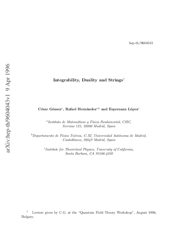
 Esperanza Lopez